Path Diffusion, part I

Abstract.

This paper investigates the position (state) distribution of the single step binomial (multi-nomial) process on a discrete state / time grid under the assumption that the velocity process rather than the state process is Markovian. In this model the particle follows a simple multi-step process in velocity space which also preserves the proper state equation of motion. Many numerical numerical examples of this process are provided. For a smaller grid the probability construction converges into a correlated set of probabilities of hyperbolic functions for each velocity at each state point. It is shown that the two dimensional process can be transformed into a Telegraph equation and via transformation into a Klein-Gordon equation if the transition rates are constant. In the last Section there is an example of multi-dimensional hyperbolic partial differential equation whose numerical average satisfies Newton’s equation. There is also a momentum measure provided both for the two-dimensional case as for the multi-dimensional rate matrix.

Introduction

This paper investigates the position (state) distribution of the single step binomial process assuming that the velocity on the node grid rather than the state process is Markovian. Under this assumption the particle steps up or down in velocity following a simple (or multi)-step process on a fixed grid with discrete time preserving the proper equation of motion. The equations of motion are defined as a joint probability per velocity and state as a function of time and state with a state transition matrix, see Section 1. The velocity rate matrix is the consequence of the Markov assumption.

The two-factor (multi-factor) solution to the binomial probability Markovian process has different types of solutions, see the numerical examples in Section 2. For very small rate transitions the final probability distribution may show the original velocity information and transport the original conditions into the future leaving a small amount of residuals. Or the rate probabilities are considerable strongly re-bunching the distribution into something that looks like a Gaussian process. The final distribution may therefore have individual peaks reflecting velocity distributions or if the rates are large enough it shows a central single modal distribution which listens to a mean.

For a much smaller grid and constant rates the probability equations converge into a correlated set of probabilities of hyperbolic functions for each velocity in state point. The two dimensional case can be transformed into a Telegraph equation for the state density which can be transformed into a Klein-Gordon equation if the transition rates are constant. An average velocity from the state can be defined as well as Section 3 and Section 5 show.

This equation can be done in two velocity spaces or in an infinite number is a set of diffusion equations of them. Both for the two-dimensional applications and the multi-dimensional case a forward and a backward velocity can be found as Section III and Section V show. In the last Section there is multi-dimensional hyperbolic partial differential equation whose average satisfies Newton’s equation.

1. The Construction

Equation

To construct the process consider the discrete space, discrete time grid as defined in Figure  1. The process is given by the nodes

$$x(t) =m\Delta x,m=...,-1,0,1,2,...$$

$$t =0,h,2h,...$$

where $\Delta x$ is a small space grid size (vertical) and $h$ is a discrete grid for the time (horizontal). Figure  1 shows a process representing a particle stepping across an infinite node grid at discrete time intervals $0,h,2h,...$. At every time the process steps up or steps down only one node from any given node in the grid. Clearly the process can step up and down many nodes at a time but for the moment consider only the simplest case.

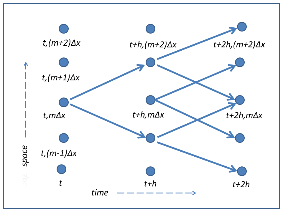
Figure 1. Typical Mid-Grid Node Transitions

If this process is Markovian in the state $x$ the probability of being in state $x(t+h)$ depends on the state $x(t)$ but not on any state before $t$. By design then a probability can be constructed on $x(t+h)=m\Delta x,m=...-1,0,1,...$ from probabilities in $x(t)$. A Gaussian or backward equation can be constructed in this fashion by considering the limit for the outcome space by scaling $\Delta x\backsim\sqrt{(}h)$ and then calculating the final distribution from increasing evolutions  [5].

However, in this paper we assume that the process is Markovian in the process velocity $(x(t),x(t+h))$ rather than the process state position $x(t)$. This means that any transition $(x(t),x(t+h))$ depends on all previous transitions $(x(t-h),x(t))$ but not on any previous transitions.

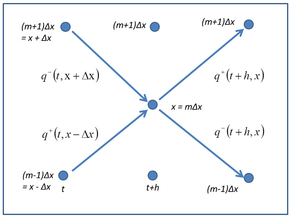
Figure 2. Node Transition Analysis

An example of this process is shown in Figure  2. If the particle resides at time $t+h$ in the node in the middle of the grid then $x(t+h)=m\Delta x=x$ for some $m$. Since it can only step up or down from this state the only possible outcomes at time point $t+2h$ are

$$x(t+2h) =x+\Delta=(m+1)\Delta x$$

or

$$x(t+2h) =x-\Delta=(m-1)\Delta x.$$

Similarly, to be in grid node $m\Delta x$ at time $t+h$ the particle must have stepped down / up from

$$x(t) =x+\Delta=(m+1)\Delta x$$

or

$$x(t) =x-\Delta=(m-1)\Delta x.$$

The grid and the joint transition probabilities for the stepping process are shown in Figure  2 for the gridpoints around $t+h,m\Delta x$.

Now let $x=m\Delta x$ in Figure  2 and let

(1.1) $$\begin{split}q^{+}(t+h,x)=P[x(t+2h)=x+\Delta x,x(t+h)=x]\\ q^{-}(t+h,x)=P[x(t+2h)=x-\Delta x,x(t+h)=x]\end{split}$$

be the up/down joint probabilities of an up or down step after the particle travels through $x$. As the velocity process is Markovian the joint process (1.1) must be dependent only on

$$q^{+}(t,x-\Delta x) =P[x(t+h)=x,x(t)=x-\Delta x]$$

$$q^{-}(t,x+\Delta x) =P[x(t+h)=x,x(t)=x+\Delta x]$$

linearly or otherwise. Notice that $q^{+}(t+h,x),q^{-}(t+h,x),q^{+}(t,x-\Delta x),q^{-}(t+h,x+\Delta x)$ are all joint distributions.

Hence the Markovian assumption requires that

(1.2) $$\begin{pmatrix}q^{+}(t+h,x)\\ q^{-}(t+h,x)\end{pmatrix}=\begin{pmatrix}1-\alpha(t,x)&\beta(t,x)\\ \alpha(t,x)&1-\beta(t,x)\end{pmatrix}\begin{pmatrix}q^{+}(t,x-\Delta x)\\ q^{-}(t,x+\Delta x)\end{pmatrix}$$

for specific constants $\alpha(t,x)$, $\beta(t,x)$. Notice that the $\alpha(t,x)$, $\beta(t,x)$ parameters do not have to be equal but must be positive and that the columns must add up to one to conserve probability. After the particle arrives in $x$ it can only step up or step down.

Probabilistically the $\alpha(t,x)$ parameters consider the probability that the particle travels downward from $x$ to $x-\Delta x$ at time $t$ after travelling up from $x-\Delta x$ to $x$ at time $t-h$. Similarly the $\beta(t,x)$ parameters consider the probability that the particle travels upward from $x$ to $x+\Delta x$ at time $t$ after travelling down from $x+\Delta x$ to $x$ at time $t-h$. Specifically

(1.3) $$\begin{split}\begin{matrix}\alpha(t,x)=P_{t}[x-\Delta,x,x-\Delta x]&\text{= probability being in $x(t)=x$ and stepping}\\ {}&{\text{down after traveling from $x(t-h)=x-\Delta$}}\\ \beta(t,x)=P_{t}[x+\Delta,x,x+\Delta x]&{\text{= probability being in $x(t)=x$ and stepping}}\\ {}&{\text{up after traveling from $x(t-h)=x+\Delta$}}.\end{matrix}\end{split}$$

Notice that as the timestep $h$ becomes smaller these curvature probabilities become smaller as well.

The probability densities $q^{+}(t,x)$, $q^{-}(t,x)$ are joint particle distributions of being in position $x(t)=x$ and moving in the ”up” or ”down” direction at the same time. So in fact the probability density $\rho(t,x)$ of the state can be defined as

$$P[x(t)=x]=\rho(t,x)=q^{+}(t,x)+q^{-}(t,x)$$

which provides the probability that the particle is in state $x$ at time $t$. Now a summation over all $x=m\Delta x$ (summing over $m$) will add up to one.

Results

Adding the two equations in (1.2) yields

$$\rho(t+h,x)=q^{+}(t+h,x)+q^{-}(t+h,x)=q^{+}(t,x-\Delta x)+q^{-}(t,x+\Delta x)$$

so that the probability of a particle being in $t+h,x$ is accumulated from the probability of the particle being in $x+\Delta$ at time $t$ stepping down and the probability of the particle being in $x-\Delta$ stepping up. This condition conserves probability specifically for the case where only up or down steps are allowed and clearly is dictated by the particle’s motion.

This equation also implies that

$$\sum_{m}\rho(t+h,m\Delta x) =\sum_{m}q^{+}(t,(m-1)\Delta x)+\sum_{m}q^{-}(t,(m+1)\Delta x)$$

$$=\sum_{m}q^{+}(t,m\Delta x)+\sum_{m}q^{-}(t,m\Delta x)$$

$$=\sum_{m}\rho(t,m\Delta x)=1$$

which shows that state probability is conserved. Also then

(1.4) $$\begin{split}&\sum_{m}q^{+}(t,m\Delta)<1\\ &\sum_{m}q^{-}(t,m\Delta)<1.\end{split}$$

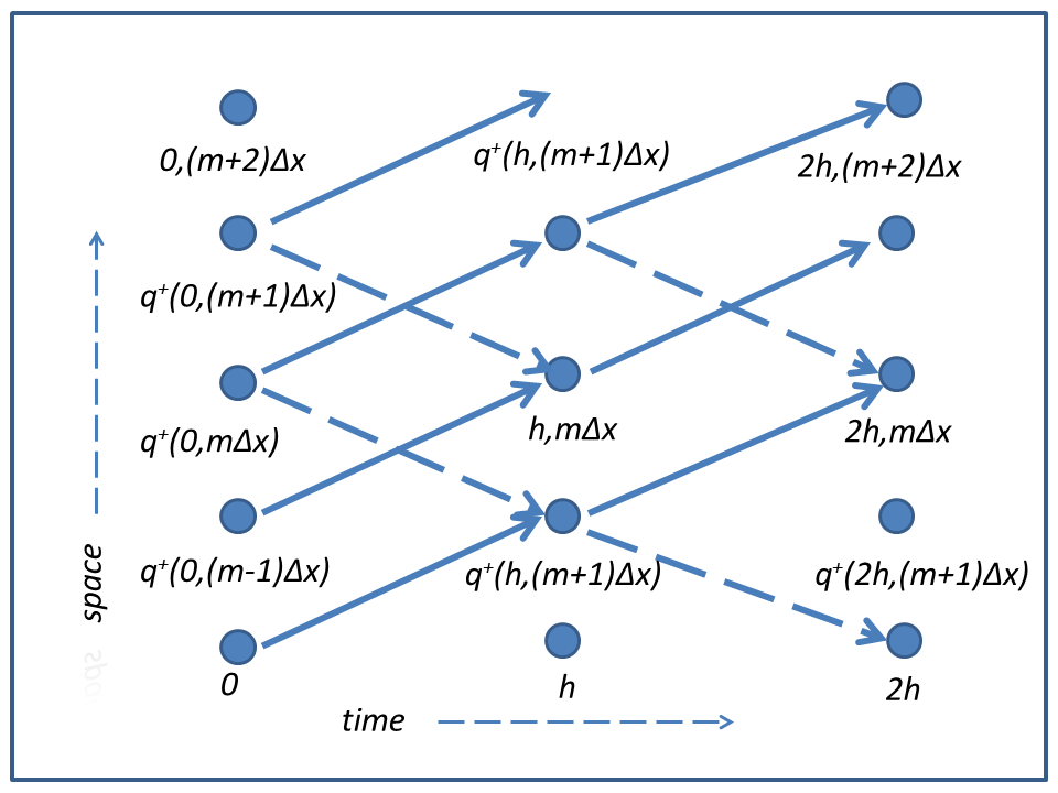
Figure 3. Initial Grid / Tree Transitions

To start the solution to (1.2) consider Figure 3 where the positive probability of transition is given solid and the downward probabilities are gridded. The first line shows the starting zero line and the starting probabilities $q^{+}(0,m\Delta x)$ for all $m$. Simultaneously there is set of initial probabilities in the downward direction $q^{-}(0,m\Delta x)$ for all $m$. The second line $q^{+}(h,m\Delta x)$ is constructed from a combination of both $q^{+}(0,m\Delta x)$ and $q^{-}(0,m\Delta x)$ using (1.2). From (1.4) it is clear that neither $q^{+}(0,m\Delta x)$ or $q^{-}(0,m\Delta x)$ are proper distributions but together they are to add to one. Hence

$$\rho(0,m\Delta x)=q^{+}(0,m\Delta x)+q^{-}(0,m\Delta x)\text{ all $m$}$$

$$q^{+}(0,m\Delta x)\geq 0\text{ all $m$}$$

$$q^{-}(0,m\Delta x)\geq 0\text{ all $m$}$$

$$\sum_{m}\left(q^{+}(0,m\Delta x)+q^{-}(0,m\Delta x)\right)=1$$

is the appropriate starting condition for the process.

If a particle residing in $x$ at time $t$ steps to $x+\Delta$ at time $t+h$ it adopts a velocity of $v^{+}=\Delta x/h=c$. Similarly if the particle steps down to $\Delta x$ it adopts a velocity of $v^{-}=-\Delta x/h=-c$. Clearly then the + and the - in the marginal densities $q^{\pm}(t,x)$ also refer to the speed of the particle passing through $x$. If there are bigger steps from $x$ where it jumps many nodes there could be speeds of $jc,j=...,-2,-1,0,1,2,...$ as multiples of the one-step particle velocity.

2. Numerical Examples

First Example, small transition probabilities

The first numerical solution is presented in Figures 4 and 5 presenting the numerical probability density solution of equation (1.2) for the case where the transition probabilities are very small ($\alpha=0.006,\beta=0.006$ per time step). The size of $\Delta x=0.3$ and the timestep $h=0.003$ so the distribution tree has a relatively high speed of $0.3/0.003=\pm 100$. The initial probability distribution at time 0 stretches from -6.9 to 6.9 over some 46 nodes.

For this case we use the initial distributions $q^{+}(0,x)$, $q^{-}(0,x)$ assuming a set of discrete Gaussian distributions so that

$$q^{+}(0,x)=q^{-}(0,x)=c_{0}e^{-\frac{x^{2}}{2\sigma^{2}}}$$

$$\rho(0,m\Delta x)=q^{+}(0,m\Delta x)+q^{-}(0,m\Delta x)$$

$$\sum_{m}\rho(0,m\Delta x)=1$$

where the constant $c_{0}$ has been chosen so that $\rho(0,m\Delta x)$ is a proper discrete distribution in the discrete parameter $m$. This distribution of $\rho(0,x)$ is shown in the center of Figure 4 for a standard deviation equal to 0.6.

The calculation grid in this is a tree starting at zero steadily enlarging for some 150 timesteps where the final time will be $t=0.45=150*0.03$. The effect of the small transition probabilities suggests that half the initial probability solutions is sent symmetrically up the grid with speed $100$ and half the initial distribution is sent down the grid at $-100$.

With 46 nodes the symmetric original initial distribution shows a distribution of $-6.9,6.9$ as the central distribution in Figure 4 shows. With the fact that the initial tree is $-6.9,6.9$ this means that the final set of nodes reaches $-45-6.9,45+6.9$ = $-51.9,51.9$. which is exactly the boundary shown for the left side and right side distribution in Figure 4. Notice that the two left and right distribution are very similar to the initial distribution but not exactly the same while the amount of probability in this distribution is less than half the initial probability density.

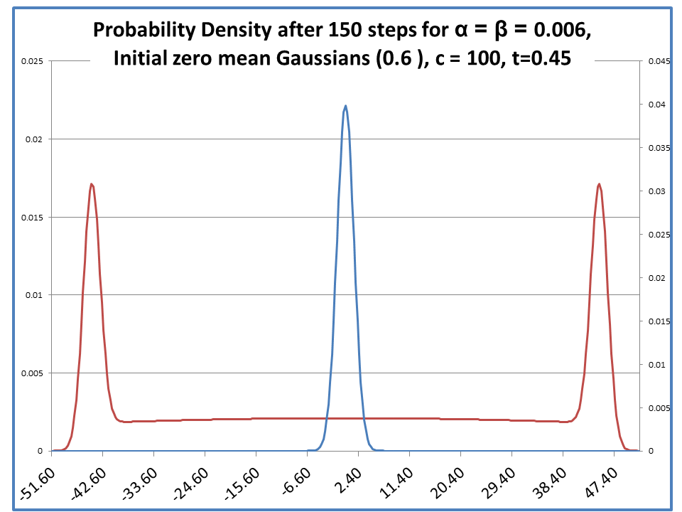
Figure 4. Initial, Final Node Densities, Small Transitions

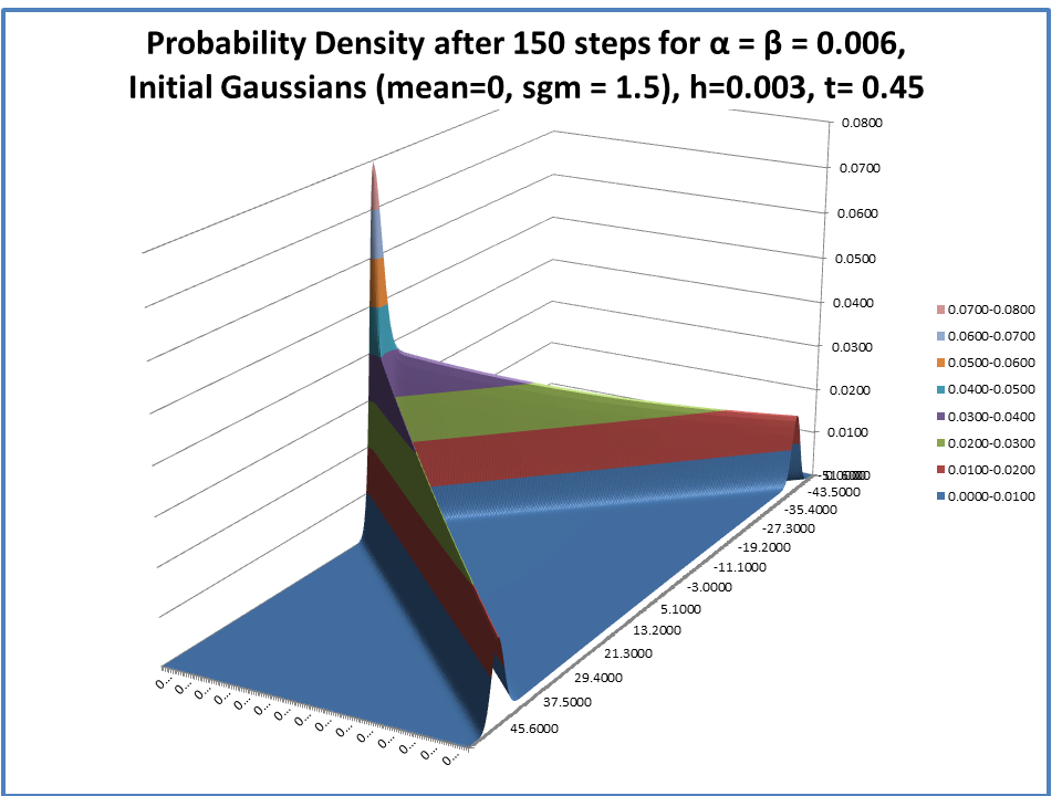
Figure 5. 3D Node Transition Travel, Small Transitions

Once the initial distributions have been determined the distribution is calculated from the difference equation (1.2) and Figure 4 shows the final distribution after 150 time steps and the initial distribution $\rho(0,x)$. Figure 5 presents a three dimensional picture of the distribution changes. The initial distribution contains all the probability which is then split in two, half of it traveling up and 100 and part of it traveling down at -100. The end distributions are slightly wider than the initial distribution. Notice that there is also a certain amount of probability assigned to the interval in between the extremes, compare Figures 4 and 5.

Physically this example shows the distribution of particles that start in about 46 nodes between -6.9 and 6.9 on the real line and then step upward or downward with about equal probability. Once the particles start moving up / down the grid the change that they change direction is small.

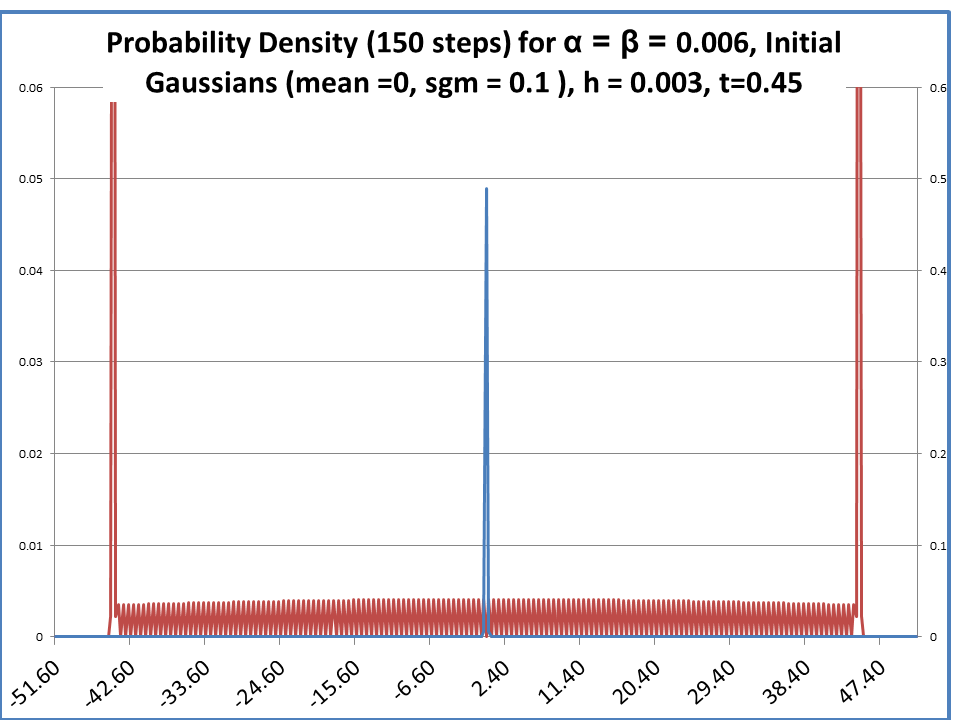
Figure 6. Extreme Narrow Initial Probability Concentration

Second Example, small transition probabilities, pointed initial conditions

A more extreme concentration version of the previous example can be created by taking the initial distribution equal to a point weight. The simulation is exactly the same as in the example above but the initial distribution now has a standard deviation of 0.1. The initial distribution distribution and the 150 step final result is shown in Figure 6. Notice that the end distribution (left and right side of Figure) have been scaled up (right hand side of the Figure) showing the final distributions of the initial conditions as in the previous example. However also notice that the final distribution between the extremes is now a clear zig-zag pattern of values.

This Figure erratic distribution pattern of probability over the final distribution is due to the fact that the particles can only step up or down. Starting in node 0 a particle can only reside on node +1 or -1 after one time step but not on node 0. Similarly after 2 steps the particle can only reside on node +2, 0, -2 but not on nodes +1 or -1. The final result is a superimposed interference pattern which is an artifact of the fact that the particles are not allowed to remain on certain nodes and the concentrated initial distribution. As a result there is a noticeable difference in the distribution between adjacent nodes and the difference in value creates the interference. Taking a wider initial distribution removes this mixture and recreates a more continuous final distribution.

Interestingly the interference patterns depend on the initial distributions and the transition probabilities. Given the small transition probabilities the interference decreases with increasing initial distribution variance around the 0.25 - 0.3 standard deviation. This was determined by looking at Figure 6 while varying the standard deviation of the initial distribution.

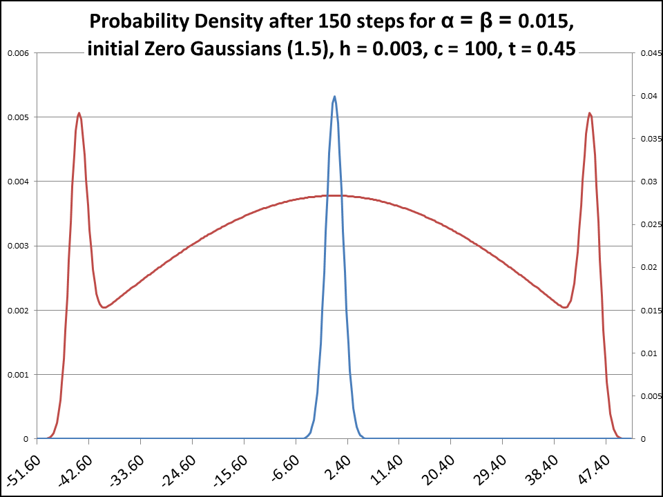
Figure 7. Initial, Final Node Densities, Mixed Transitions

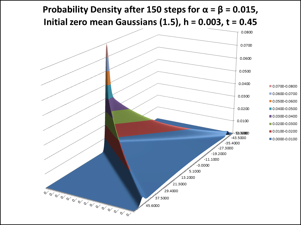
Figure 8. 3D Node Transition Travel, Mixed Transitions

Third Example, mixed transition probabilities, symmetric

In the next example the transition probabilities are much larger so that part of the probability travels to the edges following the speed requirements but the remaining part of the distribution is settled in the middle. Figures 7 and 8 show a more balanced case again where the standard deviation of the initial distributions is put back to 1.5 but now the transition probabilities are increased to $\alpha=0.015=1.5\%$, $\beta=0.015=1.5\%$. Much of the final distribution is away from the solution bound -45.00 and 45.00 but some of the particles still end there.

Comparing Figures 8 with Figure 5 it is clear that a larger part of the distribution is located between the extreme nodes. Also the size of the distributions at the -51.9 and 51.9 extreme points is now quite a bit smaller reflecting the probability diffusion into the region between the extremes. As Figure 7 suggests the final distribution looks vaguely Gaussian but has substantial ”ears” at the extremes.

Fourth Example, large transition probabilities, non-symmetric

Figures 9, 10 show an example of the grid building for the case where the transition probabilities are much bigger and also not symmetrical. In this case the extreme distributions will disappear as they can only be obtained if the particles do not deviate from the straight path which is unlikely given the 150 steps. Also the recombining steps generate a distribution that is much more centered in the middle while showing a curve in the direction of the largest transition parameter.

Figures 9 shows the initial and final 150 step distribution. The final distribution looks Gaussian but has increased in standard deviation and moved off-center. The initial distribution was centered around zero and then migrated to 10.99 at time 0.45 while the standard deviation started with 1.5 as per our initial distribution and then changed to about 16.2 at the final time $t=0.45$. Due to the distribution spreading there is always an increase in the standard deviation and in the next Section we will show how this depends on time and probabilities.

The migration of the mean is difficult to estimate and is not equal to $150*(\alpha-\beta)*\Delta x$. The $\alpha$ and $\beta$ determine the curvature of the path but they say nothing about the mean motion or the ”up” or ”down” probability. This ”up” and ”down” probability effectively determines the movement of the mean but they cannot be easily determined without calculation and for these cases they are time dependent.

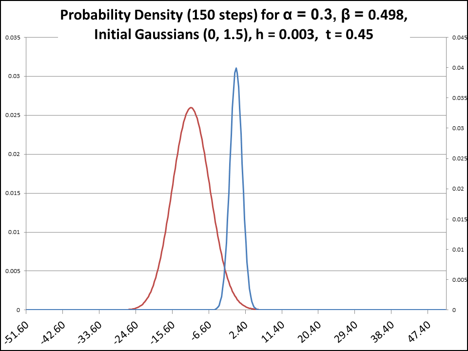
Figure 9. Initial, Final Node Densities, Large Transitions

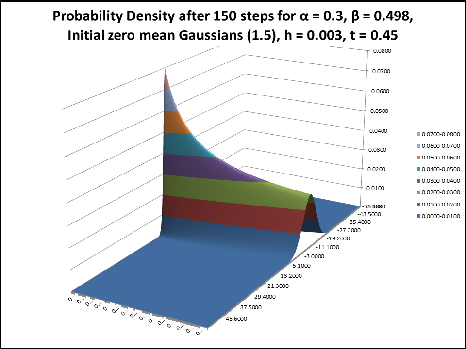
Figure 10. 3D Node Transition Travel, Large Transitions

3. Continuous Case

Continuous Equation

Assuming an appropriate limit leaving $\Delta/h\rightarrow c$ and in proportion it is possible to transform equation (1.2) to a continuous equation. Assume that $\Delta/h=c$ which means that the speed of the particle is always constant. So then a particle moves only with speed $c$ or equal $-c$. Additionally assume that the probabilities $\alpha$ and $\beta$ behave as rates getting smaller with $h$ so that

$$\alpha(t,x) \rightarrow\alpha(t,x)h$$

$$\beta(t,x) \rightarrow\beta(t,x)h.$$

Then a two factor jump process can be constructed for the position probability of the particle.

To apply these limits to equation (1.2) insert $c$ and change the probabilities as rates. Expand the $\Delta x$ terms to find that

$$\begin{pmatrix}q^{+}(t+h,x)\\ q^{-}(t+h,x)\end{pmatrix}=\begin{pmatrix}1-\alpha(t,x)h&\beta(t,x)h\\ \alpha(t,x)h&1-\beta(t,x)h\end{pmatrix}\begin{pmatrix}q^{+}(t,x)-\Delta x\frac{\partial}{\partial x}q^{+}(t,x)+O(\Delta^{2}x)\\ q^{-}(t,x)+\Delta x\frac{\partial}{\partial x}q^{-}(t,x)+O(\Delta^{2}x)\end{pmatrix}$$

so that

$$\begin{pmatrix}q^{+}(t+h,x)\\ q^{-}(t+h,x)\end{pmatrix}= \begin{pmatrix}1-\alpha(t,x)h&\beta(t,x)h\\ \alpha(t,x)h&1-\beta(t,x)h\end{pmatrix}\begin{pmatrix}q^{+}(t,x)\\ q^{-}(t,x)\end{pmatrix}$$

$$+\Delta x\begin{pmatrix}1-\alpha(t,x)h&\beta(t,x)h\\ \alpha(t,x)h&1-\beta(t,x)h\end{pmatrix}\begin{pmatrix}-\frac{\partial}{\partial x}q^{+}(t,x)\\ \frac{\partial}{\partial x}q^{-}(t,x)\end{pmatrix}.$$

Notice that in the last part of the equation there are terms $h\Delta x$ that can be ignored as they are small. Retaining the main terms yields

$$\begin{split}\begin{pmatrix}q^{+}(t+h,x)-q^{+}(t,x)\\ q^{-}(t+h,x)-q^{-}(t,x)\end{pmatrix}=&h\begin{pmatrix}-\alpha(t,x)&\beta(t,x)\\ \alpha(t,x)&-\beta(t,x)\end{pmatrix}\begin{pmatrix}q^{+}(t,x)\\ q^{-}(t,x)\end{pmatrix}\\ &+\Delta x\begin{pmatrix}-\frac{\partial}{\partial x}q^{+}(t,x)\\ \frac{\partial}{\partial x}q^{-}(t,x)\end{pmatrix}\end{split}$$

so dividing by $h$ and calculating the limit yields

(3.1) $$\begin{split}\frac{\partial}{\partial t}\begin{pmatrix}q^{+}(t,x)\\ q^{-}(t,x)\end{pmatrix}=&\begin{pmatrix}-\alpha(t,x)&\beta(t,x)\\ \alpha(t,x)&-\beta(t,x)\end{pmatrix}\begin{pmatrix}q^{+}(t,x)\\ q^{-}(t,x)\end{pmatrix}+c\frac{\partial}{\partial x}\begin{pmatrix}-q^{+}(t,x)\\ q^{-}(t,x)\end{pmatrix}\end{split}$$

taking $\Delta\downarrow 0$,$h\downarrow 0$ and setting $\Delta/h=c$. The term $h^{2}$ is ignored as they are an order of magnitude smaller.

Reorganizing this yields

(3.2) $$\begin{split}\frac{\partial q^{+}(t,x)}{\partial t}+c\frac{\partial q^{+}(t,x)}{\partial x}+\alpha(t,x)q^{+}(t,x)&=\beta(t,x)q^{-}(t,x)\\ \frac{\partial q^{-}(t,x)}{\partial t}-c\frac{\partial q^{-}(t,x)}{\partial x}+\beta(t,x)q^{-}(t,x)&=\alpha(t,x)q^{+}(t,x)\end{split}$$

which is a set of coupled convection equations flowing the probability over the grid. This type of equation looks like a hyperbolic one-dimensional Telegraph Equation for the behavior of voltage and current waves in a lossy transmission line though the signs are different  [7] or  [13]. In this case there are only initial conditions in the form of initial densities $q^{+}(0,x)$, $q^{-}(0,x)$ and there are usually no Dirichlet type boundary conditions (time dependent fixed $x$ boundaries). Dirichlet boundaries only arise if the probability flow is restricted in state over time.

Telegraph Equation

Equation (3.2) can be recast in a two dimensional Telegraph equation. As before let $\rho(t,x)=q^{+}(t,x)+q^{-}(t,x)$ and define $\phi(t,x)=q^{+}(t,x)-q^{-}(t,x)$ then equations (3.1) and (3.2) can be rewritten as

$$\begin{split}&\frac{\partial}{\partial t}\rho(t,x)=-c\frac{\partial}{\partial x}\phi(t,x)\\ &\frac{\partial}{\partial t}\phi(t,x)=-c\frac{\partial}{\partial x}\rho(t,x)-2\alpha(t,x)q^{+}(t,x)+2\beta(t,x)q^{-}(t,x)\end{split}$$

or substituting $q^{+}(t,x)=(\rho(t,x)+\phi(t,x))/2$ and $q^{-}(t,x)=(\rho(t,x)-\phi(t,x))/2$ this reduces to

(3.3) $$\frac{\partial}{\partial t}\rho(t,x)=-c\frac{\partial}{\partial x}\phi(t,x)$$

(3.4) $$\frac{\partial}{\partial t}\phi(t,x)=-c\frac{\partial}{\partial x}\rho(t,x)-\epsilon(t,x)\rho(t,x)-\gamma(t,x)\phi(t,x)$$

where $\gamma(t,x)=\alpha(t,x)+\beta(t,x)$ and $\epsilon(t,x)=\alpha(t,x)-\beta(t,x)$.

If $\alpha(t,x)=\alpha,\beta(t,x)=\beta$ (reducing $\gamma(t,x)$ and $\epsilon(t,x)$ to constants) this equation can be further reduced. Denote $\gamma(t,x)=\gamma,\epsilon(t,x)=\epsilon$ and taking the time derivative in (3.3) equation into the second equation (3.4) yields

$$\begin{split}\frac{\partial^{2}}{\partial t^{2}}\rho(t,x)=&-c\frac{\partial}{\partial x}\left(-c\frac{\partial}{\partial x}\rho(t,x)-\epsilon\rho(t,x)-\gamma\phi(t,x)\right)\\ =&c^{2}\frac{\partial^{2}}{\partial x^{2}}\rho(t,x)+c\epsilon\frac{\partial}{\partial x}\rho(t,x)+c\gamma\frac{\partial}{\partial x}\phi(t,x)\end{split}$$

which becomes

(3.5) $$\begin{split}\frac{\partial^{2}}{\partial t^{2}}\rho(t,x)+\gamma\frac{\partial}{\partial t}\rho(t,x)=c^{2}\frac{\partial^{2}}{\partial x^{2}}\rho(t,x)+c\epsilon\frac{\partial}{\partial x}\rho(t,x)\end{split}$$

using (3.3) on the last term in the equation.

This is a two dimensional Telegraph equation which has damping in time $t$ as well as in the spatial coordinate $x$. Notice various applications involving voltage and current waves in  [8],  [11] though these typically have Dirichlet type additional conditions. Also the Cauchy problem for the Telegraph equation based on its simulation by a one-dimensional Markov random evolution has a similar form to  [15] using Cauchy boundary conditions. There are applications of stochastic processes to biology that have generated the Telegraph Equation with Cauchy boundaries  [3].

The Telegraph equation in statistics have been proposed in the literature to describe motions of particles with finite velocities as opposed to diffusion-type models. The first contribution in this area goes back to  [6],  [12]. In  [10] and in  [2] is shown the Telegraph equations similar to (3.2) and (3.5) for local probabilities. This is more an equation for the joint probabilities rather than the conditional probabilities used in this manuscript. For a Markov process representation using Telegraph jump processes and market models see  [14].

This equation can be reduced to the damped Klein-Gordon as we will see below. Notice that in this case the initial condition requires an initial function for $\rho(t,x)$ as well as $\phi(t,x)$ satisfying (3.3) and (3.4).

Klein Gordon Equation

It is relatively straightforward to change equation (3.5) into a Klein-Gordon equation as follows.

Theorem 3.1.

To reduce equation (3.5) further assume that the solution can be written as

(3.6) $$\rho(t,x)=e^{-\frac{\epsilon}{2c}x-\frac{\gamma}{2}t}\psi(t,x)$$

for constant $\epsilon,\gamma$ then

(3.7) $$\begin{split}\frac{\partial^{2}\psi(t,x)}{\partial t^{2}}&=c^{2}\frac{\partial^{2}\psi(t,x)}{\partial x^{2}}+\eta^{2}\psi\end{split}$$

with $4\eta^{2}=4\alpha\beta=(\gamma^{2}-\epsilon^{2})$.

Proof.

Writing the state probability as

$$\rho(t,x)=e^{Ax+Bt}\psi(t,x)$$

then for the first two terms in (3.5)

$$\gamma\frac{\partial\rho(t,x)}{\partial t}=\gamma e^{Ax+Bt}\left(\frac{\partial\psi(t,x)}{\partial t}+B\psi\right)$$

$$\frac{\partial^{2}\rho(t,x)}{\partial t^{2}}=e^{Ax+Bt}\left(\frac{\partial^{2}\psi(t,x)}{\partial t^{2}}+2B\frac{\partial\psi(t,x)}{\partial t}+B^{2}\psi\right)$$

or

$$\frac{\partial^{2}\rho(t,x)}{\partial t^{2}}+\gamma\frac{\partial\rho(t,x)}{\partial t} =e^{Ax+Bt}\left(\frac{\partial^{2}\psi(t,x)}{\partial t^{2}}+(2B+\gamma)\frac{\partial\psi(t,x)}{\partial t}+(B^{2}+\gamma B)\psi\right)$$

$$=e^{Ax+Bt}\left(\frac{\partial^{2}\psi(t,x)}{\partial t^{2}}-\frac{\gamma^{2}}{4}\psi\right)$$

if we use $B=-\gamma/2$ to dispense the first derivative.

Similarly for the two terms on the right

$$c\epsilon\frac{\partial\rho(t,x)}{\partial x}=c\epsilon e^{Ax+Bt}\left(\frac{\partial\psi(t,x)}{\partial x}+A\psi\right)$$

$$c^{2}\frac{\partial^{2}\rho(t,x)}{\partial x^{2}}=c^{2}e^{Ax+Bt}\left(\frac{\partial^{2}\psi(t,x)}{\partial x^{2}}+2A\frac{\partial\psi(t,x)}{\partial x}+A^{2}\psi\right)$$

or

$$c^{2}\frac{\partial^{2}\rho(t,x)}{\partial x^{2}}+c\epsilon\frac{\partial\rho(t,x)}{\partial x} =e^{Ax+Bt}\left(c^{2}\frac{\partial^{2}\psi(t,x)}{\partial x^{2}}+(2c^{2}A+c\epsilon)\frac{\partial\psi(t,x)}{\partial x}+Ac(Ac+\epsilon)\psi\right)$$

$$=e^{Ax+Bt}\left(c^{2}\frac{\partial^{2}\psi(t,x)}{\partial x^{2}}-\frac{\epsilon^{2}}{4}\psi\right)$$

if again we use $A=-\epsilon/(2c)$ to remove the first derivative.

These two results reduce equation (3.5) to

$$\frac{\partial^{2}\psi(t,x)}{\partial t^{2}} =c^{2}\frac{\partial^{2}\psi(t,x)}{\partial x^{2}}+\frac{\gamma^{2}-\epsilon^{2}}{4}\psi=c^{2}\frac{\partial^{2}\psi(t,x)}{\partial x^{2}}+\eta^{2}\psi$$

with the definition for $\eta$ above. ∎

There are many solutions to this equation depending on the type of applications. One interesting example to be further discussed below is that the general solution to (3.7) equals

$$\psi(t,x) =AI_{0}(\xi)+BK_{0}(\xi)$$

$$\xi =\frac{\eta}{c}\sqrt{K(t,x)}$$

$$K(t,x) =c^{2}t^{2}-x^{2}$$

where $I_{0}(.),K_{0}(.)$ are first order modified Bessel functions. One particularly interesting fact is that if $\psi(t,x)$ is an equation to (3.7) then

(3.8) $$\psi^{*}\left(\frac{t-xv/c^{2}}{\sqrt{\vphantom{(}1-v^{2}/c^{2})}},\frac{x-vt}{\sqrt{\vphantom{(}1-v^{2}/c^{2})}}\right)$$

is a solution as well for an arbitrary velocity $v$.

Imagine a reasonably large mass such that $\gamma<<1$ moving with speed $v$ then using (3.8) we have that

$$\rho(t,x)=e^{-\frac{\epsilon}{2c}x-\frac{\gamma}{2}t}\psi^{*}(t,x)\approx\psi^{*}(t,x)$$

is a probability density hugging the straight path of the underlying mass moving at speed $v$. Here $\gamma$ is small because a larger mass has little dispersion so that $\gamma\approx 0$ and the $x$ term in the exponential disappears. Also it is assumed that $\epsilon$ is small assuming a very large speed of $c$. So $\epsilon/c\approx 0$ and the $x$ term from the exponential disappears and the approximation holds.

This Klein-Gordon wave equation is commonly used in relativistic quantum mechanics to find the spin-less free particle for a wave function. Equation (3.7) applies to the actual equation after adjustment and is related to tachyons [4] or transport equations [1].

Speed, Forward and Backward

To find out about the average position of a particle going through $x$ we look into the probability exiting from one node. Using Bayes on equation (1.3) and (1.2) any particle leaving state $x$ at time $t$ has a velocity of $\pm c$ with probability

$$P[x(t+h)=x+\Delta x|x(t)=x]=\frac{P[x(t+h)=x+\Delta x,x(t)=x]}{P[x(t)=x]}=\frac{q^{+}(t,x)}{\rho(t,x)}$$

$$P[x(t+h)=x-\Delta x|x(t)=x]=\frac{P[x(t+h)=x-\Delta x,x(t)=x]}{P[x(t)=x]}=\frac{q^{+}(t,x)}{\rho(t,x)}$$

because $q^{\pm}(t,x)=P[x(t+h)=x\pm\Delta x,x(t)=x]$ is the joint probability, see (1.2), (1.3).

Hence the expectation of the exiting speed of the particle conditional on residing in $x$ at time $t$ equals

(3.9) $$v(t,x)=c\frac{(q^{+}(t,x)-q^{-}(t,x))}{\rho(t,x)}=c\frac{\phi(t,x)}{\rho(t,x)}$$

where $\phi(t,x)=q^{+}(t,x)-q^{-}(t,x)$. Hence the difference between the two densities $q^{+}(t,x)$,$q^{-}(t,x)$ also has a physical interpretation.

For the backward velocity consider the steps in the grid ending in $x(t)=x$ before taking the average. So by definition using Bayes again

$$P[x(t-h)=x+\Delta x|x(t)=x]=\frac{P[x(t-h)=x+\Delta x,x(t)=x]}{P[x(t)=x]}=\frac{q^{+}(t-h,x+\Delta x)}{\rho(t,x)}$$

$$P[x(t-h)=x-\Delta x|x(t)=x]=\frac{P[x(t-h)=x-\Delta x,x(t)=x]}{P[x(t)=x]}=\frac{q^{+}(t-h,x-\Delta x)}{\rho(t,x)}$$

now concentrating on the probability of ending up in $x$ coming from $x+\Delta x$ with velocity $-c$ or coming from $x-\Delta x$ with velocity $c$.

It is possible to define a backward velocity and an acceleration using an inversion of equation (1.2).

Theorem 3.2.

The hyperbolic two dimensional hyperbolic equation (3.2) which has forward velocity (3.9) also has an acceleration equal to

$$a_{t}(x) =\lim_{h\downarrow 0}\frac{v(t,x)-v^{-}(t,x)}{h}=-c\epsilon(t,x)-v(t,x)\gamma(t,x)$$

with $v^{-}(t,x)$ defined as the speed of the particle that ends in $x$ - the backward velocity.

Proof.

Using the Bayes argument as before the backward velocity becomes

$$v^{-}(t,x)=c\left(P[x(t-h)=x-\Delta x|x(t)=x]-P[x(t-h)=x+\Delta x|x(t)=x]\right)$$

which equals

$$v^{-}(t,x) =c\left(\frac{P[x(t-h)=x-\Delta x,x_{t}=x]}{P[x_{t}=x]}-\frac{P[x(t-h)=x+\Delta x,x_{t}=x]}{P[x_{t}=x]}\right)$$

$$=c\left(\frac{q^{+}(t-h,x-\Delta x)}{\rho(t,x)}-\frac{q^{-}(t-h,x+\Delta x)}{\rho(t,x)}\right)$$

$$=\frac{c}{\rho(t,x)}\left(q^{+}(t-h,x-\Delta x)-q^{-}(t-h,x+\Delta x)\right).$$

This can be simplified by means of inverting equation (1.2) since then

(3.10) $$\begin{split}\begin{pmatrix}q^{+}(t-h,x-\Delta x)\\ q^{-}(t-h,x+\Delta x)\end{pmatrix}&=\begin{pmatrix}1-\alpha(t-h,x)h&\beta(t-h,x)h\\ \alpha(t-h,x)h&1-\beta(t-h,x)h\end{pmatrix}^{-1}\begin{pmatrix}q^{+}(t,x)\\ q^{-}(t,x)\end{pmatrix}\\ &=\frac{1}{D_{t-h}}\begin{pmatrix}1-\beta(t-h,x)h&-\beta(t-h,x)h\\ -\alpha(t-h,x)h&1-\alpha(t-h,x)h\end{pmatrix}\begin{pmatrix}q^{+}(t,x)\\ q^{-}(t,x)\end{pmatrix}\\ &=\frac{1}{D_{t-h}}\begin{pmatrix}(1-h\beta(t-h,x))q^{+}(t,x)-h\beta(t-h,x)q^{-}(t,x)\\ -hq^{+}(t,x)\alpha(t-h,x)+(1-h\alpha(t-h,x))q^{-}(t,x)\end{pmatrix}\\ &=\frac{1}{D_{t-h}}\begin{pmatrix}q^{+}(t,x)-h\beta(t-h,x)\rho(t,x)\\ q^{-}(t,x)-h\alpha(t-h,x)\rho(t,x)\end{pmatrix}\end{split}$$

with the matrix determinant

$$D_{t-h} =(1-h\beta(t-h,x))(1-h\alpha(t-h,x))-h^{2}\beta(t-h,x)\alpha(t-h,x)$$

$$=\left(1-h(\beta(t-h,x)+\alpha(t-h,x))\right)=1-h\gamma(t-h,x).$$

Substituting this into equation (3.10) yields

$$v^{-}(t,x) =\frac{c}{\rho(t,x)}\left(q^{+}(t-h,x-\Delta x)-q^{-}(t-h,x+\Delta x)\right)$$

$$=\frac{c}{D_{t-h}\rho(t,x)}\left(q^{+}(t,x)-q^{-}(t,x)+h(\alpha(t-h,x)-\beta(t-h,x))\rho(t,x)\right)$$

$$=\frac{v(t,x)+ch\epsilon(t-h,x)}{D_{t-h}}=\frac{v(t,x)+hc\epsilon(t-h,x)}{1-h\gamma(t-h,x)}$$

using $\epsilon(t-h,x)=\alpha(t-h,x)-\beta(t-h,x)$.

Now expanding in rising orders of $h$

(3.11) $$\begin{split}v^{-}(t,x)&=\frac{v(t,x)+ch\epsilon(t-h,x)h}{1-h\gamma(t-h,x)}\\ &=(v(t,x)+ch\epsilon(t-h,x))(1+h\gamma(t-h,x)+...)\\ &=v(t,x)+c\epsilon(t-h,x)h+v(t,x)\gamma(t-h,x)h+...\end{split}$$

or in the limit

$$a_{t}(x) =\lim_{h\downarrow 0}\frac{v(t,x)-v^{-}(t,x)}{h}=-c\epsilon(t,x)-v(t,x)\gamma(t,x)$$

using $\epsilon(t,x)=\lim_{h\downarrow 0}(\alpha(t-h,x)-\beta(t-h,x)$, $\gamma(t,x)=\lim_{h\downarrow 0}(\alpha(t-h,x)+\beta(t-h,x))$. ∎

This is therefore a practical definition of acceleration through point $x$. Notice that the matters of limits and continuity for $\alpha(t,x)$, $\beta(t,x)$ are technical issues which have been ignored in this proof.

4. Solutions

Equation (3.2), the Telegraph equation (3.5) and the Klein-Gordon equations (3.7) have solutions for the case where there are specific initial Cauchy conditions. This involves distributions for the initial condition and the initial velocity.

The situation here is slightly different from the usual applications in electromagnetism, investment or previous probabilistic studies in that the distribution is defined as the sum of $q^{+}(t,x)$, $q^{-}(t,x)$ and no initial distribution is normally provided for the Telegraph equation.

However, it is quite straightforwar5d to show the following.

Theorem 4.1.

Using the notation from Theorem 3.1 with $\eta^{2}=(\beta^{2}-\alpha^{2})/4)$ with initial conditions

$$\rho(0,x)=q^{+}(0,x)+q^{-}(0,x)$$

then the solution to (3.2) and (3.5) is given by

(4.1) $$\begin{split}q^{+}(t,x)=e^{-\frac{\epsilon}{2c}x-\frac{\gamma}{2}t}\psi^{+}(t,x)\\ q^{-}(t,x)=e^{-\frac{\epsilon}{2c}x-\frac{\gamma}{2}t}\psi^{-}(t,x)\\ \rho(t,x)=q^{+}(t,x)+q^{-}(t,x)\end{split}$$

where

$$\psi^{\pm}(t,x)= \frac{\left(\psi^{\pm}(x+ct)+\psi^{\pm}(x-ct)\right)}{2}+\frac{ct\eta}{2}\int_{x-ct}^{x+ct}\psi^{\pm}(z)\frac{I_{0}(\frac{\eta}{c}\xi(t,x-z))}{\xi(t,x-z)}dz$$

with

$$\psi^{\pm}(x) =e^{\frac{\epsilon}{2c}x}q^{\pm}(0,x)$$

$$\xi =\sqrt{c^{2}t^{2}-x^{2}}.$$

Proof.

Equation (3.7) presents the Klein-Gordon equation for a function of the overall space probability density $\rho(t,x)$. This was derived from (3.6) and (3.5). However, it is possible to use the equations to show that the same Telegraph equation (3.5) applies for $\phi(t,x)$. However in that case the initial conditions would be different.

Since both the addition $\rho(t,x)$ and the difference $\phi(t,x)$ satisfy the Telegraph equation their difference and their addition also satisfies the Telegraph equation (3.5). Since $q^{+}(t,x)=(\rho(t,x)+\phi(t,x))/2$, $q^{-}(t,x)=(\rho(t,x)-\phi(t,x))/2$ also satisfy the Telegraph equation once transformed with the exponential (3.6) relation they also satisfy the Klein-Gordon equation. Hence $\rho(t,x),\phi(t,x),q^{+}(t,x),q^{-}(t,x)$ all satisfy the Klein-Gordon equation though with different conditions.

The solution to the Klein-Gordon equation under the Cauchy conditions is

$$\psi(t,x)= \frac{(\psi(x+ct)+\psi(x-ct))}{2}+\frac{ct\eta}{2}\int_{x-ct}^{x+ct}\psi(\xi)\frac{I_{0}(\frac{\eta}{c}\sqrt{\vphantom{(}c^{2}t^{2}-(x-\xi)^{2}})}{\sqrt{\vphantom{(}c^{2}t^{2}-(x-\xi)^{2}}}d\xi$$

$$+\frac{1}{2c}\int_{x-ct}^{x+ct}\theta(\xi)K_{0}(m\sqrt{\vphantom{(}c^{2}t^{2}-(x-\xi)^{2}}))d\xi$$

where

$$\psi(0,x)=\psi(x)$$

$$\frac{\partial}{\partial t}\psi(0,x)=\theta(x).$$

Given the fact that we do not have a conditional derivative we can drop the $\theta(t,x)$ term above and put in the appropriate initial condition for the individual densities. Using (3.6) these initial condition are

$$q^{+}(0,x) =e^{-\frac{\epsilon}{2c}x}\psi^{+}(x)$$

or

$$q^{-}(0,x) =e^{-\frac{\epsilon}{2c}x}\psi^{-}(x)$$

hence inverting this yields $\psi^{\pm}(0,x)=e^{\frac{\epsilon}{2c}x}q^{\pm}(0,x)$ which are the initial conditions provided in (4.1).

The resulting equation then is a solution to the Klein-Gordon equation using the initial condition for $q^{+}(0,x),q^{-}(0,x)$. To find the solution for the Telegraph equation we need the exponential as in (3.6) for either initial case which explains the equations in (4.1). The equations for $q^{=}(t,x)$, $q^{-}(t,x)$ are one factor equations and so the procedure above should find a unique solution. ∎

On the other hand if $\gamma$ and $c$ become large so that $\gamma,c>>1$ then equation (3.5) can be rewritten as

(4.2) $$\begin{split}\frac{\partial}{\partial t}\rho(t,x)=\frac{c^{2}}{\gamma}\frac{\partial^{2}}{\partial x^{2}}\rho(t,x)+\frac{c\epsilon}{\gamma}\frac{\partial}{\partial x}\rho(t,x)-\frac{1}{\gamma}\frac{\partial^{2}}{\partial t^{2}}\rho(t,x)\end{split}$$

and the last term in the limit vanishes (since $1/\gamma<<1$) to yield

$$\begin{split}\frac{\partial}{\partial t}\rho(t,x)=\frac{c^{2}}{\gamma}\frac{\partial^{2}}{\partial x^{2}}\rho(t,x)+\frac{c\epsilon}{\gamma}\frac{\partial}{\partial x}\rho(t,x)\end{split}$$

which is a diffusion equation with variance $\sigma^{2}=\dfrac{c^{2}}{\gamma}$ and drift $-\dfrac{c\epsilon}{\gamma}$.

In fact, if in addition $\alpha=\beta$ then $\epsilon=\alpha-\beta=0$ and $\gamma=2\alpha$ so equation (4.2) reduces to

$$\begin{split}\frac{\partial}{\partial t}\rho(t,x)=\frac{c^{2}}{\gamma}\frac{\partial^{2}}{\partial x^{2}}\rho(t,x)=\frac{c^{2}}{2\alpha}\frac{\partial^{2}}{\partial x^{2}}\rho(t,x)\end{split}$$

which is the quintessential diffusion.

The result is not surprising since a large $\gamma$ indicates a very high probability of switching velocities in any state $x$. The typical Brownian path has a very high (infinite) velocity (here equal to $c$) but changes directions at a very high (infinitely large) rate.

Some properties can be seen more or less from equation (3.5).

Theorem 4.2.

For small $\gamma$ the velocity of the mean remains equal to its initial value while for large $\gamma$ and large $c$ the mean speed of the mean becomes

$$v_{0}=-\frac{c\epsilon}{\gamma}.$$

Also

$$E[x^{2}(t)]\approx\frac{2c^{2}t}{\gamma}+E[x(t)]^{2}$$

for $\gamma>>1$ and $\gamma t>>1$.

Proof.

Integrating equation (3.5) shows that

$$\frac{d^{2}}{dt^{2}}\int_{-\infty}^{\infty}x\rho(t,x)dx+\gamma\frac{d}{dt}\int_{-\infty}^{\infty}x\rho(t,x)dx=-c\epsilon$$

so that

$$\frac{d^{2}}{dt^{2}}E[x(t)]+\gamma\frac{d}{dt}E[x(t)]=-c\epsilon.$$

The solution to this is straightforward

(4.3) $$v_{t}=\frac{d}{dt}E[x(t)]=-\frac{c\epsilon}{\gamma}+\left(v_{0}+\frac{c\epsilon}{\gamma}\right)e^{-\gamma t}$$

where

$$v_{0}=\frac{d}{dt}E[x(0)]$$

a simple reference to the initial velocity. Clearly then the particle has initial velocity $v_{0}$ but after a fair time $\gamma t<<1$ we get $v_{\infty}=-\frac{c\epsilon}{\gamma}$.

Integrating (4.3) once once more yields

$$E[x(t)] =E[x(0)]-\frac{c\epsilon t}{\gamma}+\left(v_{0}+\frac{c\epsilon}{\gamma}\right)\frac{1-e^{-\gamma t}}{\gamma}$$

$$\approx E[x(0)]-\frac{c\epsilon t}{\gamma}\approx E[x(0)]+v_{\infty}t$$

as long as $\gamma>>1$ and $\gamma t>>1$.

Equation (3.5) also shows that

$$\frac{d^{2}}{dt^{2}}\int_{-\infty}^{\infty}x^{2}\rho(t,x)dx+\gamma\frac{d}{dt}\int_{-\infty}^{\infty}x^{2}\rho(t,x)dx=2c^{2}-2c\epsilon E[x(t)]$$

so that

(4.4) $$\frac{d}{dt}E[x^{2}(t)]=e^{-\gamma t}E[x^{2}(0)]+\frac{2c^{2}}{\gamma}\left(1-e^{-\gamma t}\right)-2c\epsilon\int_{0}^{t}e^{-\gamma(t-s)}E[x(s)]ds$$

The last term in this equation becomes

$$\int_{0}^{t}e^{-\gamma(t-s)}E[x(s)]ds \approx\int_{0}^{t}e^{-\gamma(t-s)}\left(E[x(0)]-\frac{c\epsilon s}{\gamma}\right)ds$$

$$=\frac{E[x(0)]}{\gamma}\left(1-e^{-\gamma t}\right)-\frac{c\epsilon}{\gamma}\left(\frac{t}{\gamma}-\frac{1-e^{-\gamma t}}{\gamma^{2}}\right)$$

$$\approx\frac{E[x(0)]}{\gamma}-\frac{c\epsilon t}{\gamma^{2}}$$

so then equation (4.4) becomes

$$\frac{d}{dt}E[x^{2}(t)] \approx\frac{2c^{2}}{\gamma}-\frac{2c\epsilon E[x(0)]}{\gamma}+\frac{2c^{2}\epsilon^{2}t}{\gamma^{2}}$$

$$\approx\frac{2c^{2}}{\gamma}-\frac{2c\epsilon}{\gamma}\left(E[x(0)]-\frac{c\epsilon t}{\gamma}\right)$$

$$\approx\frac{2c^{2}}{\gamma}+v_{\infty}\left(E[x(0)]+v_{\infty}t\right)$$

$$\approx\frac{2c^{2}}{\gamma}+\frac{d}{dt}E[x(t)]^{2}$$

so that

$$E[x^{2}(t)]\approx\frac{2c^{2}t}{\gamma}+E[x(t)]^{2}$$

∎

This result shows that the distribution is consistent with a Gaussian diffusion as the variance increases with time while the remaining terms are of order $1/\gamma$.

However, if $\alpha(t,x)$ and $\epsilon(t,x)$ depend on the state $x$ and time $t$ explicitly then a different approach is required.

5. Multi-dimensional Case

Infinite Dimensional Equation

It is easy to generalize the previous algorithm in (1.2) by introducing both more states to step into and more states to come from. In the multi-dimensional case the state $x(t)$ is connected to many other states $x(t+h)=x+j\Delta x$. Define

$$q^{j}(t,x)=P[x(t+h)=x+j\Delta x,x(t)=x],\text{ for }j=...,-1,0,1,...$$

as the set of joint speed and position probabilities generalizing (1.1). To generalize (1.3) let probability being in $x(t+h)=x$ and stepping to $x+k\Delta x$ at $t+h$ after traveling from $x(t)=x+j\Delta x$ at $t-h$ equal

$$\begin{matrix}\omega_{jk}(t,x)=P_{t}[x+j\Delta x,x,x+k\Delta x]\end{matrix}$$

with $\sum_{j}\omega_{jk}=1$. Then the equivalent to (1.2) reduces to

(5.1) $$q^{j}(t+h,x)=\sum_{k}\omega_{jk}q^{k}(t,x-k\Delta x)$$

for $j,k=...,-1,0,1,...$. This implies that $q^{j}(t,x)$ is the joint distribution of being in position $x_{t}=x$ and making a step the size $j\Delta x,j=...,-1,0,1,...$. Notice that this means that the particle has a velocity of $v_{j}=j\Delta x/h=jc,j=...,-1,0,1,...$.

As a result $\sum_{j}q^{j}(t,x)=\rho(t,x)$ is the marginal probability of the particle residing in $x$ and so adding the equations in (5.1) yields

$$\rho(t+h,x)=\sum_{j}q^{j}(t+h,x)$$

so that

$$\sum_{n}\rho(t+h,n\Delta x) =\sum_{n}\sum_{j}q^{j}(t,x-n\Delta x)$$

$$=\sum_{j}\sum_{n}q^{j}(t,x-n\Delta x)$$

$$=\sum_{j}q^{j}(t,x)=1$$

which shows that state probability is conserved.

To create an equation we now assume that the $\omega$ matrix becomes a rate similar to the $\alpha$, $\beta$ in Section 3. Substitute $\omega_{jk}\rightarrow\delta_{jk}+h\omega_{jk}$ then equation (5.1) becomes

(5.2) $$q^{j}(t+h,x)=\sum_{k}\left(\delta_{jk}+h\omega_{jk}\right)q^{k}(t,x-k\Delta x)$$

for all appropriate indices $j=...,-1,0,1,...$. Now $\omega_{jk}$ is a rate matrix which has positive values for all off-diagonal elements and has negative values on the diagonal with $\sum_{j}\omega_{jk}=0$.

To apply this to equation (5.1) expand on the small terms $\Delta x$ and write

$$q^{j}(t+h,x)=\sum_{k}(\delta_{jk}+\omega_{jk}h)\left(q^{k}(t,x)-k\Delta x\frac{\partial}{\partial x}q^{k}(t,x)\right)$$

where $\sum_{j}\omega_{jk}=0$ for all $k$.

Retaining the main terms then yields

$$q^{j}(t+h,x)-q^{j}(t,x)= h\sum_{k}\omega_{jk}q^{k}(t,x)-j\Delta x\frac{\partial}{\partial x}q^{j}(t,x)$$

and so finally in the limit

(5.3) $$\begin{split}\frac{\partial}{\partial t}q^{j}(t,x)+v_{j}\frac{\partial}{\partial x}q^{j}(t,x)=\sum_{k}\omega_{jk}q^{k}(t,x),\text{ $j=...,-1,0,1,...$}\end{split}$$

were $v_{j}=j\Delta x/h$ as above and where the terms $v_{j}h$ and $h^{2}$ can be ignored as they are an order of magnitude smaller. This is a set of coupled advection equations.

Speed, Forward

The definition of average speed $v(t,x)$ translates directly from equation (3.9)

(5.4) $$v(t,x)=\frac{\sum_{j}v_{j}q^{j}(t,x)}{\rho(t,x)}=c\frac{\sum_{j}jq^{j}(t,x)}{\rho(t,x)}$$

which also implies that

$$\sum_{j}v_{j}q^{j}(t,x)=v(t,x)\rho(t,x).$$

Notice here we use the definition $\Delta x/h=c$.

Using this equation it is clear that

$$\frac{\partial}{\partial t}\rho(t,x)+\frac{\partial}{\partial x}\sum_{j}v_{j}q^{j}_{t}(x)=0$$

so that

(5.5) $$\frac{\partial}{\partial t}\rho(t,x)+\frac{\partial}{\partial x}\left(v(t,x)\rho(t,x)\right)=0.$$

This equation is the continuity equation which is true for any distribution no matter what the choices are for velocities $v_{k}$, model size or otherwise. The remaining models depend on the choices of $\omega$ and for some matrix configuration we can simulate the Newtonian system.

Theorem 5.1.

Let the probability matrix in (5.3) equal

$$w=\begin{pmatrix}\ddots&\alpha&0&0\\ \beta&-\lambda&\alpha&0\\ 0&\beta&-\lambda&\alpha\\ 0&0&\beta&-\lambda\\ 0&0&0&\beta\end{pmatrix}$$

with $\lambda=\alpha+\beta$ and let

(5.6) $$\alpha-\beta=\frac{1}{c}\frac{\partial V}{\partial x}$$

then

$$\frac{\partial^{2}}{\partial t^{2}}E\left[x(t)\right]=E\left[\frac{\partial V}{\partial x}\right]$$

so that the average motion of the particle follows Newton’s equation.

Proof.

Consider that equation (5.3) the per velocity distribution and multiply each row with $v_{k}$. Then sum over the equation to get

$$\frac{\partial}{\partial t}\sum_{j}v_{j}q^{j}_{t}(x)+\frac{\partial}{\partial x}\sum_{j}v^{2}_{j}q^{j}_{t}(x)=\sum_{jk}v_{j}\omega_{jk}q^{k}(t,x)$$

with equation

$$w=\begin{pmatrix}\ddots&\alpha&0&0\\ \beta&-(\alpha+\beta)&\alpha&0\\ 0&\beta&-(\alpha+\beta)&\alpha\\ 0&0&\beta&-(\alpha+\beta)\\ 0&0&0&\beta\end{pmatrix}.$$

Take $v_{k}=k\Delta x/h=kc$ then for all $k$ we have

$$\sum_{j}v_{j}\omega_{jk}=\sum_{j}cj\omega_{jk} =c\left(\alpha(k-1)-(\alpha+\beta)k+\beta(k+1)\right)$$

$$=-c(\alpha-\beta)=-\frac{\partial V}{\partial x}$$

As a result the right hand side of equation (5.5) changes

$$\frac{\partial}{\partial t}\sum_{j}v_{j}q^{j}_{t}(x)+\frac{\partial}{\partial x}\sum_{j}v^{2}_{j}q^{j}_{t}(x)=-c\epsilon\rho(t,x)=-\frac{\partial V}{\partial x}\rho(t,x)$$

or using the continuity equation (5.5) we find

$$\frac{\partial}{\partial t}(v(t,x)\rho(t,x))+\frac{\partial}{\partial x}\sum_{j}v^{2}_{j}q^{j}_{t}(x)=-\frac{\partial V}{\partial x}\rho(t,x).$$

Notice that the second term is a state derivative in $x$ so the average over this - the integral over $x$ vanishes. As a result now

$$\frac{\partial^{2}}{\partial t^{2}}E\left[x(t)\right] =\frac{\partial}{\partial t}\int_{-\infty}^{\infty}x\frac{\partial\rho(t,x)}{\partial t}dx=\frac{\partial}{\partial t}\int_{-\infty}^{\infty}-x\frac{\partial v(t,x)\rho(t,x)}{\partial x}dx$$

$$=\frac{\partial}{\partial t}\int_{-\infty}^{\infty}v(t,x)\rho(t,x)dx=-c\int_{-\infty}^{\infty}\left(\sum_{jk}v_{j}\omega_{jk}q^{k}(t,x)\right)dx$$

$$=\int_{-\infty}^{\infty}\left(\sum_{k}\frac{\partial V}{\partial x}q^{k}(t,x)\right)dx=\int_{-\infty}^{\infty}\frac{\partial V}{\partial x}\rho(t,x)dx=E\left[\frac{\partial V}{\partial x}\right].$$

∎

Notice that in this example there is no uniqueness for the choices of $\alpha$ and $\beta$. The actual form of the transaction matrix is not clear and the actual form in which these parameters depend on the potential is surprising.

After this example let us take a look at the energy embedded in equation (5.3) with rate choices (5.6).

Theorem 5.2.

Using the probability matrix defined in Theorem 5.1 and using the definition of potential in (5.3) then

$$\frac{1}{2}E\left[\sum_{j}v_{j}^{2}q^{j}(t,x)\right]=\frac{1}{2}\int\sum_{j}v_{j}^{2}q^{j}(t,x)dx$$

is the average kinetic energy of the particle and

$$\frac{\partial}{\partial t}\left[\frac{1}{2}E\left[\sum_{j}v_{j}^{2}q^{j}(t,x)\right]dx+E\left[V\right]\right]=\frac{c^{2}}{2}(\alpha+\beta).$$

Proof.

Using again (5.3) multiply each row with $v_{k}^{2}=k^{2}c^{2}$ and sum over the equation to get

$$\frac{\partial}{\partial t}\sum_{j}v_{j}^{2}q^{j}_{t}(x)+\frac{\partial}{\partial x}\sum_{j}v^{3}_{j}q^{j}_{t}(x)=\sum_{jk}v_{j}^{2}\omega_{jk}q^{k}(t,x).$$

Take $v_{k}^{2}=k^{2}c^{2}$ then for all $k$ we have

$$\sum_{j}v_{j}^{2}\omega_{jk}=\sum_{j}c^{2}j^{2}\omega_{jk} =c^{2}\left(\alpha(k-1)^{2}-(\alpha+\beta)k^{2}+\beta(k+1)^{2}\right)$$

$$=-2kc^{2}(\alpha-\beta)+c^{2}(\alpha+\beta)$$

$$=-2ck\frac{\partial V}{\partial x}+c^{2}(\alpha+\beta)$$

so then

$$\frac{\partial}{\partial t}\sum_{j}v_{j}^{2}q^{j}_{t}(x)+\frac{\partial}{\partial x}\sum_{j}v^{3}_{j}q^{j}_{t}(x) =\sum_{k}\left(-2ck\frac{\partial V}{\partial x}+c^{2}(\alpha+\beta)\right)q^{k}(t,x)$$

$$=-2c\frac{\partial V}{\partial x}\sum_{k}kq^{k}(t,x)+c^{2}(\alpha+\beta)\rho(t,x)$$

$$=-2\frac{\partial V}{\partial x}v(t,x)\rho(t,x)+c^{2}(\alpha+\beta)\rho(t,x).$$

Now notice that

$$\frac{\partial}{\partial t}E\left[V\right] =\frac{\partial}{\partial t}\int V\rho(t,x)dx=\int V\frac{\partial}{\partial t}\rho(t,x)dx$$

$$=-\int V\frac{\partial}{\partial x}\left(v(t,x)\rho(t,x)\right)dx=\int\frac{\partial V}{\partial x}v(t,x)\rho(t,x)dx.$$

Taking expectation on both sides noticing that the partial $x$ term vanishes so that

$$\frac{1}{2}\int\frac{\partial}{\partial t}\sum_{j}v_{j}^{2}q^{j}_{t}(x)dx+\int\frac{\partial V}{\partial x}v(t,x)\rho(t,x)dx=\frac{c^{2}}{2}(\alpha+\beta)\int\rho(t,x)dx$$

or

$$\frac{\partial}{\partial t}\left[\frac{1}{2}E\left[\sum_{j}v_{j}^{2}q^{j}_{t}(x)\right]dx+E\left[V\right]\right]=\frac{c^{2}}{2}(\alpha+\beta).$$

∎

So the energy defined in the system evaporates at a rate $(\alpha+\beta)c^{2}/2$ depending on the choices of the system as long the difference between $\alpha$ and $\beta$ is proportional to the differential of the potential. A logical choice for rate parameters becomes

$$\alpha =\theta+\frac{1}{2c}\frac{\partial V}{\partial x}$$

$$\beta =\theta-\frac{1}{2c}\frac{\partial V}{\partial x}$$

where for the moment it is assumed that

$$\left|\frac{1}{2c}\frac{\partial V}{\partial x}\right|<<\theta.$$

In this case $(\alpha+\beta)c^{2}/2=\theta c^{2}$.

Substituting this choice into (5.3) for the $\omega$ matrix becomes

$$w =\theta\begin{pmatrix}-2&1&&&\\ 1&-2&&&\\ &&\ddots&&\\ &&&-2&1\\ &&&1&-2\end{pmatrix}+\frac{1}{2c}\begin{pmatrix}0&\frac{\partial V}{\partial x}&&&\\ -\frac{\partial V}{\partial x}&0&\frac{\partial V}{\partial x}&&\\ &&\ddots&&\\ &&-\frac{\partial V}{\partial x}&0&\frac{\partial V}{\partial x}\\ &&&-\frac{\partial V}{\partial x}&0\end{pmatrix}$$

$$=\theta\widetilde{D}+\frac{1}{2c}\widetilde{\Gamma}$$

with obvious definitions for the $NxN$ sized symmetric matrix $\widetilde{D}$ and the equal-sized antisymmetric matrix $\widetilde{\Gamma}$.

As a result

$$\frac{\partial}{\partial t}q^{j}(t,x)+v_{j}\frac{\partial}{\partial x}q^{j}(t,x)=\sum_{k}\left(\theta\widetilde{D}_{jk}+\frac{1}{2c}\widetilde{\Gamma}_{jk}\right)q^{k}(t,x),\text{ $j=-N,...,-1,0,1,...,N$}$$

for the symmetric and antisymmetric matrices above. Notice that for this case the size of the equations has been constrained to $2N+1$.

More concise form, speed

It is possible to reduce the size of the original equation by a certain amount though this may be detrimental to the simplicity of the transition matrix.

Theorem 5.3.

Let

(5.7) $$\psi^{j}(t,x)=\mathcal{H}_{j}(t)q^{j}(t,x)=e^{v_{j}t\frac{\partial}{\partial x}}q^{j}(t,x)$$

with $\mathcal{H}_{j}(t)$ is the translation operator

(5.8) $$\mathcal{H}_{j}(t)=e^{v_{j}t\frac{\partial}{\partial x}}\text{ $j=...,-1,0,1,...$}$$

for all velocities $v_{j},j=...,-1,0,1,...$. Then

$$\frac{\partial}{\partial t}\psi^{j}(t,x)=\sum_{k}\left(\mathcal{H}_{j}(t)\omega_{jk}\mathcal{H}^{-1}_{k}(t)\right)\psi^{k}(t,x)$$

where

$$\mathcal{H}_{j}(t)\omega_{jk}\mathcal{H}^{-1}_{k}(t)=e^{v_{j}t\frac{\partial}{\partial x}}\omega_{jk}e^{-v_{k}t\frac{\partial}{\partial x}}$$

for all combinations of $j,k=...,-1,0,1,....$.

Proof.

Using equation (5.7) with operator (5.8) the first part of (5.3) can be written as

$$\frac{\partial}{\partial t}q^{j}(t,x)+v_{j}\frac{\partial}{\partial x}q^{j}(t,x)=\mathcal{H}^{-1}_{j}(t)\frac{\partial}{\partial t}\mathcal{H}_{j}(t)q^{j}(t,x),\text{ $j=...,-1,0,1,...$}$$

where $\mathcal{H}_{j}(t)$ is the translation operator

$$\mathcal{H}_{j}(t)=e^{v_{j}t\frac{\partial}{\partial x}}\text{ $j=...,-1,0,1,...$}$$

for all velocities $v_{j},j=...,-1,0,1,...$.

This operator translates the argument in a function since for any test function $f=f(t,x)$

$$\mathcal{H}_{j}(t)f(t,x)=f(t+v_{j}t,t).\text{ $j=...,-1,0,1,...$}$$

Also

$$\mathcal{H}_{j}(t)\mathcal{H}_{k}(t) =\mathcal{H}_{k}(t)\mathcal{H}_{j}(t),\text{ $j=...,-1,0,1,...$}$$

$$\mathcal{H}^{-1}_{j}(t) =e^{-v_{j}t\frac{\partial}{\partial x}}.\text{ $j=...,-1,0,1,...$}$$

$$\frac{\partial}{\partial t}\mathcal{H}_{j}(t) =v_{j}\frac{\partial}{\partial x}\mathcal{H}_{j}(t)=v_{j}\mathcal{H}_{j}(t)\frac{\partial}{\partial x}.\text{ $j=...,-1,0,1,...$}$$

Applying this to equation (5.3) yields

$$\frac{\partial}{\partial t}\mathcal{H}_{j}(t)q^{j}(t,x)=\sum_{k}\mathcal{H}_{j}(t)\omega_{jk}\mathcal{H}^{-1}_{k}(t)\mathcal{H}_{k}(t)q^{k}(t,x)$$

which is equivalent to

$$\frac{\partial}{\partial t}\psi^{j}(t,x)=\sum_{k}\mathcal{H}_{j}(t)\omega_{jk}\mathcal{H}^{-1}_{k}(t)\psi^{k}(t,x)$$

with

$$\psi^{j}(t,x)=\mathcal{H}_{j}(t)q^{j}(t,x)=e^{v_{j}t\frac{\partial}{\partial x}}q^{j}(t,x).$$

∎

The other element is the energy flow through this example.

Theorem 5.4.

In this case

$$a_{t}(x) =\lim_{h\downarrow 0}\frac{v(t,x)-v^{-}(t,x)}{h}=-c\epsilon(t,x)$$

where $v(t,x)$ and $v^{-}(t,x)$ are the forward and backward energies in the system.

Proof.

To find the equivalent of (3.11) consider (5.1) in the small $h$ limit. Invert (5.2) to get

(5.9) $$q^{k}(t-h,x-v_{k}h)=\sum_{j}\left(\delta_{jk}+h\omega_{jk}\right)^{-1}q^{j}(t,x)$$

for again $k=...,-1,0,1,...$. Writing

$$\delta_{jk}+h\omega_{jk}=(I+h\omega)_{jk}$$

the inverse can be written as

$$(I+h\omega)^{-1}(I+h\omega)=I$$

and so for small $h$

$$(I+h\omega)^{-1}\approx I-h\omega.$$

Now

$$v^{-}(t,x)=\sum_{j}v_{j}P[x(t-h)=x-j\Delta x|x_{t}=x]$$

or

$$v^{-}(t,x) =\sum_{j}v_{j}\frac{q^{+}(t-h,x-j\Delta x)}{\rho(t,x)}$$

$$=\sum_{j}v_{j}\sum_{k}\frac{\left(\delta_{jk}+h\omega_{jk}\right)^{-1}q^{k}(t,x)}{\rho(t,x)}$$

$$\approx\sum_{j}v_{j}\sum_{k}\frac{\left(\delta_{jk}-h\omega_{jk}\right)q^{k}(t,x)}{\rho(t,x)}$$

$$\approx\sum_{j}v_{j}\frac{\left(q^{j}(t,x)-h\sum_{k}\omega_{jk}\right)q^{k}(t,x)}{\rho(t,x)}$$

$$\approx\sum_{j}v_{j}\frac{q^{j}(t,x)}{\rho(t,x)}-h\frac{\sum_{jk}v_{j}\omega_{jk}q^{k}(t,x)}{\rho(t,x)}$$

$$=v(t,x)+hc\epsilon$$

so acceleration through node state $x$ can be defined as

$$a(t,x)=\frac{v(t,x)-v^{-}(t,x)}{h}=-c\epsilon.$$

∎

So what is interesting is that in more dimensions the inverse velocity is a simplification of the expression derived in Theorem 3.2.

6. Conclusion

Section 1 showed the distribution for the position (state) distribution of the single step binomial process assuming that the velocity on the node grid rather than the state process is Markovian. The result is a set of joint velocity distributions related to a rate matrix.

The final distribution may show the original velocity information and for sufficient small rates and relatively small initial densities transport the original conditions into the final distribution. As the numerical example shows if the initial distribution widen and the rates increase the distribution focusses around the probabilistic drift in a single modal distribution. On the other hand for extreme small rates and a very focussed initial distribution the final density shows variations.

For a much smaller grid and constant rates the probability equations converge into a correlated set of probabilities of hyperbolic functions for each velocity in state point. The two dimensional case can be transformed into a Telegraph equation for the state density which can be transformed into a Klein-Gordon equation if the transition rates are constant. An average velocity from the state can be defined as well as Section III and Section IV show.

This equation can be done in two velocity spaces or in an infinite number is a set of diffusion equations of them. Both for the two-dimensional applications and the multi-dimensional case a forward and a backward velocity can be found as Section III and Section V show. In the last Section there is multi-dimensional hyperbolic partial differential equation whose average satisfies Newton’s equation.

References

• [1] Anno, P.D., Klein Gordon Acoustics Theory, Thesis, Coloradon School of Mines (1993).
• [2] Boguna, M., Porra‘J.M., Masoliver J, Generalization of the persistent random walk to dimensions greater than 1, Physical Review E 58 (6) (Dec 1998).
• [3] Codling, E.A., Plank, M.J., Benhamou, S., Random Walk in Biology, Journal of Royal Society Interface 5 (25) 813-834.
• [4] Feinberg, G, The Possibility of Faster Than Light, Physical Review 159, Volume 5 (1967).
• [5] Feller, W, An Introduction to Probability Theory and Its Applications, John Wiley and Sons, Volume I and II (1966, 1971).
• [6] Goldstein, S, On diffusion by discontinuous movements and the telegraph equation, Quarter Journal Mechanics Applied Mathematics 4 (129-156).
• [7] Harrington. R.F., Time-Harmonic Electromagnetic Fields, McGraw-Hill (1961).
• [8] Hosseini, M.M., Tauseef Mohyud-Din, S, Hosseini, S.M. and Heydari, M., Study on Hyperbolic Telegraph Equations by Using Homotopy Analysis Method, Studies in Nonlinear Sciences 1, (2) (2010) 50-56.
• [9] Ibe, O.C. Elements of Random Walk and Diffusion Processes, John Wiley Series in Operational Research and Operational Science, John Wiley (2013).
• [10] Iacus, S.M., Statistical analysis of the inhomogeneous telegrapher s process, Cornell University Library arXiv.org, arxiv Engine, http:/arxiv.org/abs/math/0011059v1 (2000).
• [11] Javidi, M., Nyamoradi, N., Numerical solution of telegraph equation using LT inversion Technique, International Journal of Advanced Mathematical Sciences, 1 (2) (2013) 64-77.
• [12] Kac, M., A stochastic model related to the Telegraphers equation, Rocky Mountain Journal Mathematics 4 (1974) 497-509. Reprinted from: M. Kac, Some stochastic problems in physics and mathematics, Colloquium lectures in the pure and applied sciences, No. 2, hectographed, Field Research Laboratory, Socony Mobil Oil Company, Dallas, TX (1956) 102-122.
• [13] Mittal, R.C., Bhatia, R. Numerical solution to second order one dimensional Telegraph Equation by cubic B-spline collocation method, Applied Mathematics and Computation 220, (2013) 496-506.
• [14] Ratanov, N., Telegraph processes with jump diffusion and complete market models, Cornell University Library arXiv.org, http://arxiv.org/pdf/1311.5464.pdf (2013).
• [15] Samoilenko, I.V., Turbin, A.F. A probability method for the solution of the telegraph equation with real-analytic initial conditions, Ukrainian Mathematical Journal 52 (8) (2000).