Error Decay of (almost) Consistent Signal Estimations
from Quantized Gaussian Random Projections

Abstract

This paper provides new error bounds on consistent reconstruction methods for signals observed from quantized random projections. Those signal estimation techniques guarantee a perfect matching between the available quantized data and a new observation of the estimated signal under the same sensing model. Focusing on dithered uniform scalar quantization of resolution $\delta>0$, we prove first that, given a Gaussian random frame of $\mathbb{R}^{N}$ with $M$ vectors, the worst-case $\ell_{2}$-error of consistent signal reconstruction decays with high probability as $O(\tfrac{N}{M}\log\tfrac{M}{\sqrt{N}})$ uniformly for all signals of the unit ball $\mathbb{B}^{N}\subset\mathbb{R}^{N}$. Up to a log factor, this matches a known lower bound in $\Omega(N/M)$ and former empirical validations in $O(N/M)$. Equivalently, if $M$ exceeds a minimal number of frame coefficients growing like $O(\tfrac{N}{\epsilon_{0}}\log\tfrac{\sqrt{N}}{\epsilon_{0}})$, any vectors in $\mathbb{B}^{N}$ with $M$ identical quantized projections are at most $\epsilon_{0}$ apart with high probability. Second, in the context of Quantized Compressed Sensing with $M$ Gaussian random measurements and under the same scalar quantization scheme, consistent reconstructions of $K$-sparse signals of $\mathbb{R}^{N}$ have a worst-case error that decreases with high probability as $O(\tfrac{K}{M}\log\tfrac{MN}{\sqrt{K}^{3}})$ uniformly for all such signals. Finally, we show that the proximity of vectors whose quantized random projections are only approximately consistent can still be bounded with high probability. A certain level of corruption is thus allowed in the quantization process, up to the appearance of a systematic bias in the reconstruction error of (almost) consistent signal estimates.

1 Introduction

Since the advent of the digital signal processing era and of analog-to-digital converters, an intense field of research has been concerned by the non-linear sensing model

$$\boldsymbol{q}=\mathcal{Q}[\boldsymbol{A}\boldsymbol{x}]\in\mathcal{J},$$ (1)

where $\boldsymbol{A}\in\mathbb{R}^{M\times N}$ is a matrix representing a linear transformation of a signal $\boldsymbol{x}$ taken in some bounded subset $\mathcal{K}$ of $\mathbb{R}^{N}$, and $\mathcal{Q}$ stands for a quantization of $\boldsymbol{A}\boldsymbol{x}$ that maps $\boldsymbol{A}\mathcal{K}:=\{\boldsymbol{A}\boldsymbol{u}:\boldsymbol{u}\in\mathcal{K}\}\subset\mathbb{R}^{M}$ to a finite set of vectors $\mathcal{J}\subset\mathbb{R}^{M}$, e.g., encoded over a given number of bits [17, 7].

The bounded space $\mathcal{K}$ containing generally an infinite number of signals, the model (1) is of course lossy and $\boldsymbol{x}$ cannot be recovered exactly from $\boldsymbol{q}$. Quantifying this loss of information as a function of both the signal reconstruction method and of the key elements $\boldsymbol{A}$, $N$, $M$, $\mathcal{K}$ and $\mathcal{Q}$ has been therefore the topic of many studies at the frontier of information theory, high-dimensional geometry, signal processing and statistics.

The general model (1) is for instance the one adopted in Quantized Compressed Sensing (QCS) [11, 7, 20], where the signal $\boldsymbol{x}$ is assumed sparse or compressible in an orthonormal basis $\boldsymbol{\Psi}$ of $\mathbb{R}^{N}$, and the sensing matrix is generated randomly, e.g., from Gaussian random ensembles [10]. When $M\geqslant N$, Eq. (1) is also a model for frame coefficient quantization (FCQ) of signals in $\mathbb{R}^{N}$, i.e., when the coefficients $\boldsymbol{A}\boldsymbol{x}=(\boldsymbol{a}_{1}^{T}\boldsymbol{x},\cdots,\boldsymbol{a}_{M}^{T}\boldsymbol{x})^{T}$ of $\boldsymbol{x}$ in an overcomplete frame of $\mathbb{R}^{N}$ are quantized in $\boldsymbol{q}=\mathcal{Q}(\boldsymbol{A}\boldsymbol{x})\in\mathcal{J}$, $\boldsymbol{A}=(\boldsymbol{a}_{1},\cdots,\boldsymbol{a}_{M})^{T}$ representing the matrix whose row set $\{\boldsymbol{a}_{j}\in\mathbb{R}^{N}:1\leqslant j\leqslant M\}$ collects the frame vectors [14, 15, 3].

In this work, we restrict the analysis of (1) to a scalar, regular and uniform quantizer. The quantization $\mathcal{Q}$ is then a scalar operation applied componentwise on vectors; its 1-D quantization cells $\mathcal{Q}^{-1}[c]=\{\lambda:\mathcal{Q}[\lambda]=c\}\subset\mathbb{R}$ are convex and have all the same size (or resolution) $\delta>0$. Other quantization procedures have been studied for (1) and we refer the reader for instance to [7] for a review of scalar and $\Sigma\Delta$-quantization [18] in the QCS literature, to [4] for a theoretical analysis of non-regular scalar quantizers, to [30, 25] for the use of non-regular binned quantization, or to [29] for an example of vector quantization by frame permutation. As realized in [18, 16, 7], we also assume that the “variability” of the components of $\boldsymbol{A}\boldsymbol{x}$, also measured by their variance, does not change with $M$. This is critical for defining a quantizer $\mathcal{Q}$ of constant resolution when $M$ increases.

Many studies have addressed the model (1) by observing that the distortion induced by quantization compared to a linear model $\boldsymbol{A}\boldsymbol{x}$ is the one of an additive measurement noise $\boldsymbol{n}=\mathcal{Q}[\boldsymbol{A}\boldsymbol{x}]-\boldsymbol{A}\boldsymbol{x}$ with $n_{i}\in[-\delta/2,\delta/2]$, i.e.,

$$\boldsymbol{q}=\boldsymbol{A}\boldsymbol{x}+\boldsymbol{n}.$$ (2)

When the resolution is small compared to the standard deviation of each component of $\boldsymbol{A}\boldsymbol{x}$, i.e., under the high resolution assumption [17, 7, 20], or if a random dithering is added prior to quantization [17], each component of the noise can be assumed as uniformly distributed within $[-\delta/2,\delta/2]$. This allows one to bound the power of this noise, i.e., $\mathbb{E}(\|\boldsymbol{n}\|^{2})=M\delta^{2}/12$ and $\|\boldsymbol{n}\|^{2}\leqslant{\textstyle\frac{1}{12}}\,\delta^{2}(M+\zeta\sqrt{M})$ with high probability for $\zeta=O(1)$ (see, e.g.,  [20]).

In the case of QCS, when a general noise $\boldsymbol{n}$ of bounded power $\|\boldsymbol{n}\|\leqslant\varepsilon$ corrupts the compressive observation of a sparse signal $\boldsymbol{x}$ as in (2), a worst-case reconstruction error that follows

$$\|\boldsymbol{x}-{\boldsymbol{x}}^{*}\|=O(\varepsilon/\sqrt{M}),$$

can be reached by various reconstruction methods (e.g., Basis Pursuit DeNoise [12, 10] or Iterative Hard Thresholding [2]) as soon as a suitably rescaled sensing matrix $\frac{1}{\sqrt{M}}\boldsymbol{A}$ respects the restricted isometry property (RIP) [10].

Thus, when the compressive observations of a $K$-sparse signal undergo uniform scalar quantization, it is then expected that, with high probability, $\|\boldsymbol{x}-{\boldsymbol{x}}^{*}\|=O(\delta)$ by setting $\varepsilon^{2}={\textstyle\frac{1}{12}}\,\delta^{2}(M+\zeta\sqrt{M})$. The constancy of this error with respect to $M$ is also known as the classical error limit of the pulse code modulation scheme (PCM) in CS [18].

However, most of the reconstruction techniques enforce a $\ell_{2}$-norm fidelity with $\boldsymbol{q}$, e.g., by imposing $\|\boldsymbol{A}{\boldsymbol{x}}^{*}-\boldsymbol{q}\|\leqslant\varepsilon$, and the reconstructed signal is not guaranteed to be consistent with the observations, i.e., $\mathcal{Q}[\boldsymbol{A}{\boldsymbol{x}}^{*}]\neq\boldsymbol{q}$. The knowledge of the sensing model is thus not fully exploited for reconstructing $\boldsymbol{x}$ from $\boldsymbol{q}$.

In the context of signal representations using frames, it is also known that, for unit-norm frame vectors, if the frame coefficients of a signal are corrupted by an additive noise of variance $\sigma^{2}$, the linear signal estimate synthesized from the dual frame on these coefficients has a root mean square error (RMSE) lower bounded by [15, 34]

$$(\mathbb{E}\|\boldsymbol{x}-{\boldsymbol{x}}^{*}\|^{2})^{\frac{1}{2}}\geqslant N\sigma/\sqrt{M},$$

where the expectation is taken with respect to the noise. This shows that for FCQ the reconstruction error decay of such a linear reconstruction is limited to $O(N\delta/\sqrt{M})$ since $\sigma=O(\delta)$. Nevertheless, the produced solution is also inconsistent with the observations, i.e., $\boldsymbol{A}{\boldsymbol{x}}^{*}\notin\mathcal{Q}^{-1}[\boldsymbol{q}]$, as the signal synthesis reached by the dual frame $\boldsymbol{A}^{\dagger}$ amounts to solving the least-squares problem ${\boldsymbol{x}}^{*}=\operatorname*{argmin}_{\boldsymbol{u}\in\mathbb{R}^{N}}\|\boldsymbol{q}-\boldsymbol{A}\boldsymbol{u}\|^{2}=(\boldsymbol{A}^{T}\boldsymbol{A})^{-1}\boldsymbol{A}^{T}\boldsymbol{q}=\boldsymbol{A}^{\dagger}\boldsymbol{q}$, which promotes an $\ell_{2}$-norm fidelity with respect to $\boldsymbol{q}$.

This work studies a better approach for improving the reconstruction error decay in both QCS and FCQ. The proposed analysis explicitly enforces quantization consistency while reconstructing the signal, i.e., finding an estimate ${\boldsymbol{x}}^{*}\in\mathcal{K}$ such that $\mathcal{Q}[\boldsymbol{A}{\boldsymbol{x}}^{*}]=\mathcal{Q}[\boldsymbol{A}\boldsymbol{x}]$. This procedure was initially introduced in [37] for oversampled analog-to-digital conversion of bandlimited signals, or in [14] in the more general context of quantized overcomplete signal expansion. In more detail, [14] showed that, given a random model on the generation of the sensed signal, the RMSE of any reconstruction method is lower bounded by $\Omega(N/M)$. Interestingly, the same lower bound can also be obtained on the worst-case reconstruction error without requiring any random model on the source [7]. While conjectured for general frames with redundancy factor $M/N$, the combination of a tight frame formed by an oversampled Discrete Fourier Transform (DFT) with a consistent signal reconstruction reaches this lower bound, i.e., in this case the RMSE is upper bounded by $O(N/M)$ [14]. Numerically, the reconstruction errors of recovery methods based on alternate projections onto convex sets (POCS) [37, 14] or on message passing algorithms [25], have also been observed to approach $O(N/M)$ for both deterministic and random $\boldsymbol{A}$. Moreover, the Rangan-Goyal recursive algorithm [36], which enforces local consistency of the current estimate at every iteration, provides reconstruction error decaying as $\mathbb{E}(\|\boldsymbol{x}-{\boldsymbol{x}}^{*}\|^{2})=O(1/M^{2})$ for random frames, where the expectation is made on the (uniform) quantization noise [33]. More recently, Powell and Whitehouse [34] have analyzed geometrically the worst-case error of any consistent reconstruction method. As detailed in Sec. 3, they showed for instance that, for frames constructed by taking $M$ vectors picked uniformly at random over the unit sphere $\mathbb{S}^{N-1}\subset\mathbb{R}^{N}$, the expectation of this error with respect to the random frame construction decays as $O(\delta N^{3/2}/M)$.

We can also mention that consistent reconstruction methods have been applied to QCS in the high-resolution regime (i.e., for $\delta\ll 1$ when $\mathcal{K}\subset\mathbb{B}^{N}$) [13, 21, 7]; for uniform (or bounded) noise for FCQ [34]; in the extreme 1-bit QCS setting, where quantization reduces to the application of a sign operator [5, 24, 32, 31]; and even for non-regular quantization scheme in QCS [4, 6].

Compared to these former works, we highlight three important features of this paper. These are only sketched in this Introduction and we refer the reader to Sec. 2 for their precise statements.

First, we analyse the FCQ and the QCS contexts when $\boldsymbol{A}$ is generated as a Gaussian random matrix and when the scalar quantization incorporates a uniform dithering [17, 4]. As will be clear later, this dithering, which is often used to improve the statistical properties of the quantizer and is assumed to be known in signal reconstruction, allows us to leverage a geometric connection between quantized Gaussian random projections of vectors and Buffon’s needle problem [22].

Second, we provide upper bounds for the worst-case reconstruction error of consistent signal estimations, i.e., valid for the reconstruction of any vector in the signal set $\mathcal{K}$. Those bounds hold with high (and controlled) probability over the generation of both $\boldsymbol{A}$ and the dithering as soon as $M$ is large compared to the complexity of the signal space $\mathcal{K}$.

For instance, in the case of FCQ with Gaussian random frames and $\mathcal{K}=\mathbb{B}^{N}$, we show that if $M$ is bigger than a minimal value growing like $O(\frac{\delta}{\epsilon_{0}}N\log\sqrt{N}/\epsilon_{0})$, then, with high probability, the distance between any pair of vectors in $\mathcal{K}$ having consistent observations through the mapping (1) cannot be larger than $\epsilon_{0}$ (see Theorem 1). Inverting the relationship between $\epsilon_{0}$ and the minimal $M$, this establishes also that with high probability, the distance between consistent vectors decays like $O(\frac{N}{M}\log\frac{M}{\sqrt{N}})$ (see Corollary 1).

Similar bounds are also obtained in the case of QCS of bounded sparse signals when the sensing matrix is a Gaussian random ensemble. Then, with high probability, if $M$ exceeds a minimal number of measurements growing like $O(\frac{\delta}{\epsilon_{0}}K\log\frac{N}{\epsilon_{0}\sqrt{K}})$, the distance between two consistent $K$-sparse vectors cannot be larger than $\epsilon_{0}$ (see Theorem 2). Equivalently, with high probability, their distance must then decay like $O(\frac{K}{M}\log\frac{MN}{\sqrt{K}^{3}})$ (see Corollary 1).

Finally, we evaluate the impact of relaxing the consistency requirement, i.e., allowing for a certain level of inconsistent observations, on the reconstruction error of ideal estimators based on this relaxed condition. This is done by studying the proximity of two vectors of $\mathcal{K}$ when their mappings in (1) differ by no more than $r$ components. We show that if this level $r$ is constant with respect to the evolution of $M$, i.e., what we call almost perfect consistency, the previous consistency bounds are basically unchanged up to a modification by a multiplicative factor proportional to $(N+r)/N$ for FCQ and to $(K+r)/K$ for QCS (see Theorem 3). However, in the case where $r$ can reach a constant fraction of $M$, i.e., $r\leqslant\rho M$ for $\rho>0$, then, provided $\rho<1/10$, a bias impacts the proximity of two vectors in $\mathcal{K}$ differing by no more than $r$ components in their quantized mapping. With high probability, the distance between any such vectors is then smaller than the sum of two terms, one that still decays with $M$ and another that is lower bounded by $\Omega(\rho\delta)$ (see Theorem 4).

The rest of the paper is structured as follows. We start by providing the precise statement of our main results in Sec. 2. In Sec. 3, continuing the literature analysis given above, we connect our results to a few prior works that are the most connected to our study. Sec. 4 contains the proofs of our main results, while we postpone to Appendix A the proof of a key but more technical lemma, i.e., Lemma 1, that sustains both Theorem 1 and Theorem 2.

Conventions:

In the following, we will denote domain dimensions by capital roman letters, e.g.,  $M,N$. Vectors and matrices are associated to bold symbols, e.g.,  $\boldsymbol{\Phi}\in\mathbb{R}^{M\times N}$ or $\boldsymbol{u}\in\mathbb{R}^{M}$, while lowercase light letters are associated to scalar values. The identity matrix in $\mathbb{R}^{D}$ reads $\operatorname{\mathds{1}}_{D}$. The $i^{\rm th}$ component of a vector (or of a vector function) $\boldsymbol{u}$ reads either $u_{i}$ or $(\boldsymbol{u})_{i}$, while the vector $\boldsymbol{u}_{i}$ may refer to the $i^{\rm th}$ element of a set of vectors. The set of indices in $\mathbb{R}^{D}$ is $[D]=\{1,\,\cdots,D\}$ and for any $\mathcal{S}\subset[D]$ of cardinality $S=\#\mathcal{S}$, $\boldsymbol{u}_{\mathcal{S}}\in\mathbb{R}^{\#\mathcal{S}}$ denotes the restriction of $\boldsymbol{u}$ to $\mathcal{S}$. For materializing this last operation, we also introduce the linear restriction operator $\mathcal{R}_{\mathcal{S}}$ such that $\mathcal{R}_{\mathcal{S}}\boldsymbol{u}=\boldsymbol{u}_{\mathcal{S}}$, i.e., $\mathcal{R}_{\mathcal{S}}=((\operatorname{\mathds{1}}_{M})_{\mathcal{S}})^{T}$, where $\boldsymbol{B}_{\mathcal{S}}$ denotes the matrix obtained by restricting the columns of $\boldsymbol{B}\in\mathbb{R}^{D\times D}$ to those indexed in $\mathcal{S}$. For any $p\geqslant 1$, the $\ell_{p}$-norm of $\boldsymbol{u}$ is $\|\boldsymbol{u}\|_{p}=(\sum_{i}|u_{i}|^{p})^{1/p}$ with $\|\!\cdot\!\|=\|\!\cdot\!\|_{2}$. The $(N-1)$-sphere in $\mathbb{R}^{N}$ is $\mathbb{S}^{N-1}=\{\boldsymbol{x}\in\mathbb{R}^{N}:\|\boldsymbol{x}\|=1\}$ while the unit ball is denoted $\mathbb{B}^{N}=\{\boldsymbol{x}\in\mathbb{R}^{N}:\|\boldsymbol{x}\|\leqslant 1\}$. More generally, we note $\mathbb{B}_{s}^{N}(\boldsymbol{q})=\{\boldsymbol{x}\in\mathbb{R}^{N}:\|\boldsymbol{x}-\boldsymbol{q}\|\leqslant s\}$. We use the simplified notation $\mathcal{D}^{M\times N}(\eta)$ and $\mathcal{D}^{M}(\eta)$ to denote an $M\times N$ random matrix or an $M$-length random vector, respectively, whose entries are identically and independently distributed as the probability distribution $\mathcal{D}(\eta)$ of parameters $\eta=(\eta_{1},\cdots,\eta_{P})$, e.g., the standard normal distribution $\mathcal{N}(0,1)$ or the uniform distribution $\mathcal{U}([0,\delta])$. For asymptotic relations, we use the common Landau family of notations, i.e., the symbols $O$, $\Omega$ and $\Theta$ [26]. The positive thresholding function is defined by $(\lambda)_{+}:={\textstyle\frac{1}{2}}(\lambda+|\lambda|)$ for any $\lambda\in\mathbb{R}$, and $\lfloor\lambda\rfloor$ denotes the largest integer smaller than $\lambda$.

2 Main Results

Let us now develop the precise statements of our main results. In this work, we thus focus on the interplay of a uniform midrise quantizer

$$\mathcal{Q}_{\delta}(\lambda):=\delta(\lfloor\tfrac{\lambda}{\delta}\rfloor+{\textstyle\frac{1}{2}})\in\delta(\mathbb{Z}+{\textstyle\frac{1}{2}})=:\mathbb{Z}_{\delta}$$ (3)

of resolution $\delta>0$, applied componentwise on vectors, with both a Gaussian random matrix $\boldsymbol{A}=\boldsymbol{\Phi}\sim\mathcal{N}(0,1)^{M\times N}$ and a dithering $\boldsymbol{\xi}\sim\mathcal{U}^{M}([0,\delta])$. Such a dithering, which must be known at the signal reconstruction, is often used for improving the statistical properties of the quantizer by randomizing the unquantized input location inside the quantization cell [17]. As will become clear later (see Lemma 1 and its proof in Appendix A), this uniform dithering allows us also to bridge our analysis with a geometrical probability context inspired by Buffon’s needle problem [8, 22].

Consequently, given a signal $\boldsymbol{x}$ in a bounded set $\mathcal{K}\subset\mathbb{R}^{N}$, the quantized sensing scenario studied in this paper reads

$$\boldsymbol{q}=\mathcal{Q}_{\delta}[\boldsymbol{\Phi}\boldsymbol{x}+\boldsymbol{\xi}]\in\mathbb{Z}^{M}_{\delta}.$$ (4)

This is either a sensing model for QCS with a Gaussian random sensing $\boldsymbol{\Phi}$, or a quantization scheme for FCQ when the overcomplete frame is made of $M$ vectors in $\mathbb{R}^{N}$ (with $M\geqslant N$) that are randomly and independently drawn from $\mathcal{N}(0,\operatorname{\mathds{1}}_{N})$. This guarantees that they are also linearly independent with probability 1, i.e., we obtain a Gaussian random frame (GRF) of $\mathbb{R}^{N}$.

Our main objective in order to quantify the information loss in (4) while trying to estimate $\boldsymbol{x}$ is to characterize the worst-case error

$$\mathcal{E}_{\delta}(\boldsymbol{\Phi},\boldsymbol{\xi},\mathcal{K}):=\max_{\boldsymbol{x}\in\mathcal{K}}\|\boldsymbol{x}-{\boldsymbol{x}}^{*}\|$$

of any consistent reconstruction method whose output ${\boldsymbol{x}}^{*}$ is determined by the following formal program:

$$\text{find any}\ {\boldsymbol{x}}^{*}\in\mathbb{R}^{N}\text{such that}\ \mathcal{Q}_{\delta}(\boldsymbol{\Phi}{\boldsymbol{x}}^{*}+\boldsymbol{\xi})=\mathcal{Q}_{\delta}(\boldsymbol{\Phi}\boldsymbol{x}+\boldsymbol{\xi})\ \text{and}\ {\boldsymbol{x}}^{*}\in\mathcal{K}.$$ (5)

In the case of FCQ of signals in a GRF (i.e., $M\geqslant N$), we set $\mathcal{K}=\mathbb{B}^{N}$, while in the context of QCS we take $\mathcal{K}=\Sigma_{K}(\boldsymbol{\Psi})\cap\mathbb{B}^{N}$ where $\Sigma_{K}(\boldsymbol{\Psi}):=\{\boldsymbol{v}=\boldsymbol{\Psi}\boldsymbol{\alpha}\in\mathbb{R}^{N}:\|\boldsymbol{\alpha}\|_{0}\leqslant K\}$, with $\|\boldsymbol{\alpha}\|_{0}:=\#\{j\in[N]:\alpha_{j}\neq 0\}$, is the space of $K$-sparse signals in the orthonormal basis $\boldsymbol{\Psi}\in\mathbb{R}^{N\times N}$. For the sake of simplicity, we work with the canonical basis $\boldsymbol{\Psi}=\operatorname{\mathds{1}}_{N}$ with $\Sigma_{K}:=\Sigma_{K}(\operatorname{\mathds{1}}_{N})$. However, all our results can be applied to $\boldsymbol{\Psi}\neq\operatorname{\mathds{1}}_{N}$ from the rotational invariance of the Gaussian random matrix $\boldsymbol{\Phi}\sim\mathcal{N}^{M\times N}(0,1)$ in $\mathbb{R}^{N}$ [11].

We acknowledge the fact that for $\mathcal{K}=\Sigma_{K}\cap\mathbb{B}^{N}$ the program (5) is possibly NP hard, e.g., if ${\boldsymbol{x}}^{*}$ is found by minimizing the $\ell_{0}$ “norm” under the consistency constraint [28]. However, similarly to the procedure developed in [24], we are anyway interested in studying its reconstruction error, remembering that similar ideal reconstructions in CS and in QCS have often driven the determination of feasible programs [11, 38, 13, 24, 31, 20, 21].

Notice that the error $\mathcal{E}_{\delta}$ is also associated to the biggest size, with respect to all $\boldsymbol{x}\in\mathcal{K}$, of all consistency cells $\mathcal{C}_{\boldsymbol{x}}:=\{{\boldsymbol{x}}^{*}\in\mathcal{K}:\mathcal{Q}_{\delta}(\boldsymbol{\Phi}{\boldsymbol{x}}^{*}+\boldsymbol{\xi})=\mathcal{Q}_{\delta}(\boldsymbol{\Phi}\boldsymbol{x}+\boldsymbol{\xi})\}$, i.e.,

$$\mathcal{E}_{\delta}(\boldsymbol{\Phi},\boldsymbol{\xi},\mathcal{K})=\max_{\boldsymbol{x}\in\mathcal{K}}\max_{{\boldsymbol{x}}^{*}\in\mathcal{C}_{\boldsymbol{x}}}\|\boldsymbol{x}-{\boldsymbol{x}}^{*}\|,$$

which shows that the characterization of $\mathcal{E}_{\delta}$ is actually a high dimensional geometric problem, whose general formulation can be connected to the problem of finding a finite covering of $\mathcal{K}$ of minimal size [7].

Our first contribution is an upper bound on this worst-case error for consistent signal reconstruction in the context of Gaussian Random Frame Coefficient Quantization (GRFCQ).

Theorem 1 (Proximity of consistent vectors – GRFCQ case).

Let us fix $\epsilon_{0}>0$, $0<\eta<1$, $\delta>0$ and $M\geqslant N$ such that

$$M\geqslant\tfrac{4\delta\ +\ 2\epsilon_{0}}{\epsilon_{0}}\,\big{(}N\log(\tfrac{29\sqrt{N}}{\epsilon_{0}})+\log\tfrac{1}{2\eta}\big{)}.$$

Let us randomly draw a GRF $\boldsymbol{\Phi}\sim\mathcal{N}^{M\times N}(0,1)$ and a dithering $\boldsymbol{\xi}\sim\mathcal{U}^{M}([0,\delta])$. Then, with probability higher than $1-\eta$, for all $\boldsymbol{x}\in\mathcal{K}=\mathbb{B}^{N}$ sensed by (4), any solution ${\boldsymbol{x}}^{*}$ to (5) is such that $\|\boldsymbol{x}-{\boldsymbol{x}}^{*}\|\leqslant\epsilon_{0}$, or, equivalently, $\mathcal{E}_{\delta}(\boldsymbol{\Phi},\boldsymbol{\xi},\mathbb{B}^{N})\leqslant\epsilon_{0}$.

Proof.

See Sec. 4.1. ∎

As shown in Sec. 4.2, it is then straightforward to adapt Theorem 1 to quantized observations of sparse signals, i.e., to QCS.

Theorem 2 (Proximity of consistent vectors – QCS case).

Let us fix $\epsilon_{0}>0$, $0<\eta<1$, $\delta>0$ and $M$ such that

$$M\geqslant\tfrac{4\delta\ +\ 2\epsilon_{0}}{\epsilon_{0}}\big{(}2K\log(\tfrac{56N}{\sqrt{K}\epsilon_{0}})+\log\tfrac{1}{2\eta}\big{)}.$$

Let us randomly draw a Gaussian sensing matrix $\boldsymbol{\Phi}\sim\mathcal{N}^{M\times N}(0,1)$ and a dithering $\boldsymbol{\xi}\sim\mathcal{U}^{M}([0,\delta])$. Then, with probability higher than $1-\eta$, for all $\boldsymbol{x}\in\mathcal{K}=\Sigma_{K}\cap\mathcal{B}^{N}$ sensed by (4), any solution ${\boldsymbol{x}}^{*}$ to (5) is such that $\|\boldsymbol{x}-{\boldsymbol{x}}^{*}\|\leqslant\epsilon_{0}$, or, equivalently, $\mathcal{E}_{\delta}(\boldsymbol{\Phi},\boldsymbol{\xi},\Sigma_{K}\cap\mathbb{B}^{N})\leqslant\epsilon_{0}$.

Proof.

See Sec. 4.2. ∎

As a corollary of those two theorems, the asymptotic decay of $\mathcal{E}_{\delta}$ as a function of $M$, $N$, $K$, $\delta$ and of the probability $\eta$ can be established for both GRFCQ and QCS.

Corollary 1 (Proximity decay for consistent vectors).

Given $M\geqslant 0$, $0<\eta<1$, $\delta>0$ with $\delta=O(1)$, there exists two constants ${C,C^{\prime}>0}$ such that

$$\mathbb{P}\big{[}\mathcal{E}_{\delta}(\boldsymbol{\Phi},\boldsymbol{\xi},\mathbb{B}^{N})\leqslant C\big{(}\tfrac{N}{M}\log\tfrac{M}{\sqrt{N}}+\log\tfrac{1}{2\eta}\big{)}\big{]}\geqslant 1-\eta,$$ (6)

for GRFCQ, and

$$\mathbb{P}\big{[}\mathcal{E}_{\delta}(\boldsymbol{\Phi},\boldsymbol{\xi},\Sigma_{K}\cap\mathbb{B}^{N})\leqslant C^{\prime}\big{(}\tfrac{K}{M}\log(\tfrac{MN}{\sqrt{K^{3}}})+\log\tfrac{1}{2\eta}\big{)}\big{]}\geqslant 1-\eta,$$ (7)

for QCS, where these probabilities are computed with respect to both $\boldsymbol{\Phi}\sim\mathcal{N}^{M\times N}(0,1)$ and the dithering $\boldsymbol{\xi}\sim\mathcal{U}^{M}([0,\delta])$.

Proof.

See Sec. 4.1 for GRFCQ and Sec. 4.2 for QCS. ∎

Loosely speaking, this corollary says that if $\delta=O(1)$, with probability exceeding $1-\eta$,

$$\mathcal{E}_{\delta}(\boldsymbol{\Phi},\boldsymbol{\xi},\mathbb{B}^{N})=O(\tfrac{N}{M}\log\tfrac{M}{\sqrt{N}}+\log\tfrac{1}{2\eta}),$$ (8)

for GRFCQ, and

$$\mathcal{E}_{\delta}(\boldsymbol{\Phi},\boldsymbol{\xi},\Sigma_{K}\cap\mathbb{B}^{N})=O(\tfrac{K}{M}\log(\tfrac{MN}{\sqrt{K^{3}}})+\log\tfrac{1}{2\eta}),$$ (9)

for QCS. As explained in Sec. 3, this matches existing error bounds for 1-bit compressed sensing in the case of Gaussian random projections [24]. It also improves upon previous known bounds, decaying as $O(1/{\sqrt{M}})$ for linear reconstruction methods in FCQ [14] and as $O(\sqrt{{K}/{M}})$ for QCS, while a known lower bound in $\Omega({K}/{M})$ exists [7]. Our result behaves also similarly to the bound on the mean worst-case error (established with respect to $\boldsymbol{\Phi}$ and $\boldsymbol{\xi}$ in the context of our notation) of consistent reconstruction methods obtained in [34] in the case of random frames over $\mathbb{S}^{N-1}$.

Our last contribution shows that small deviations to strict consistency are also possible while keeping control of the proximity between almost-consistent vectors. This allows us to consider a moderate corruption of the sensing model (4), e.g., in the case where it suffers from a prequantization noise $\boldsymbol{n}\in\mathbb{R}^{M}$ such that, for any $\boldsymbol{x}\in\mathcal{K}$, the bound

$$\|\mathcal{Q}_{\delta}((\boldsymbol{\Phi}\boldsymbol{x}+\boldsymbol{n})+\boldsymbol{\xi})-\mathcal{Q}_{\delta}(\boldsymbol{\Phi}\boldsymbol{x}+\boldsymbol{\xi})\|_{1}\leqslant s\,\delta$$ (10)

holds with high probability for some $s>0$. In such a case, we can relax the formal reconstruction (5) and attempt to reconstruct ${\boldsymbol{x}}^{*}$ from the program:

$$\text{find any}\ {\boldsymbol{x}}^{*}\in\mathbb{R}^{N}\ \text{such that}\\ \|\mathcal{Q}_{\delta}(\boldsymbol{\Phi}{\boldsymbol{x}}^{*}+\boldsymbol{\xi})-\mathcal{Q}_{\delta}((\boldsymbol{\Phi}\boldsymbol{x}+\boldsymbol{n})+\boldsymbol{\xi})\|_{1}\leqslant s\,\delta\\ \text{and}\ {\boldsymbol{x}}^{*}\in\mathcal{K},$$ (11)

By construction, we observe that the solution ${\boldsymbol{x}}^{*}\in\mathcal{K}$ is such that

$$\|\mathcal{Q}_{\delta}(\boldsymbol{\Phi}{\boldsymbol{x}}^{*}+\boldsymbol{\xi})-\mathcal{Q}_{\delta}(\boldsymbol{\Phi}\boldsymbol{x}+\boldsymbol{\xi})\|_{1}$$

$$\leqslant\|\mathcal{Q}_{\delta}(\boldsymbol{\Phi}{\boldsymbol{x}}^{*}+\boldsymbol{\xi})-\mathcal{Q}_{\delta}((\boldsymbol{\Phi}\boldsymbol{x}+\boldsymbol{n})+\boldsymbol{\xi})\|_{1}$$

$$\quad+\|\mathcal{Q}_{\delta}((\boldsymbol{\Phi}\boldsymbol{x}+\boldsymbol{n})+\boldsymbol{\xi})-\mathcal{Q}_{\delta}(\boldsymbol{\Phi}\boldsymbol{x}+\boldsymbol{\xi})\|_{1}\leqslant 2s\delta.$$

Therefore, characterizing the robustness of (11) amounts to studying the proximity of vectors having approximately consistent quantized random projections, i.e., we have to analyse the “largest” relaxed consistency cell $\mathcal{C}^{r}_{\boldsymbol{x}}:=\{{\boldsymbol{x}}^{*}\in\mathcal{K}:\|\mathcal{Q}_{\delta}(\boldsymbol{\Phi}{\boldsymbol{x}}^{*}+\boldsymbol{\xi})-\mathcal{Q}_{\delta}(\boldsymbol{\Phi}\boldsymbol{x}+\boldsymbol{\xi})\|_{1}\leqslant r\,\delta\}$ for $r=2s>0$, through the worst-case error

$$\mathcal{E}^{r}_{\delta}(\boldsymbol{\Phi},\boldsymbol{\xi},\mathcal{K}):=\max_{\boldsymbol{x}\in\mathcal{K}}\max_{{\boldsymbol{x}}^{*}\in\mathcal{C}^{r}_{\boldsymbol{x}}}\|\boldsymbol{x}-{\boldsymbol{x}}^{*}\|.$$

As shown in the next theorem, this is done first in the case where $r=O(1)$ relatively to $M$, i.e., for “almost perfect consistency”.

Theorem 3 (Proximity decay for almost perfectly consistent vectors).

Given $M\geqslant 0$, $0<\eta<1$, $\delta>0$ with $\delta=O(1)$, and $r\in\mathbb{N}$ with $r=O(1)$, there exists two constants $C,C^{\prime}>0$ such that

$$\mathbb{P}\big{[}\mathcal{E}^{r}_{\delta}(\boldsymbol{\Phi},\boldsymbol{\xi},\mathbb{B}^{N})\leqslant C\tfrac{N+r}{M}\big{(}\log(\tfrac{M\max(N,M)}{N})+\log\tfrac{1}{2\eta}\big{)}\big{]}\geqslant 1-\eta,$$ (12)

for GRFCQ, and

$$\mathbb{P}\big{[}\mathcal{E}^{r}_{\delta}(\boldsymbol{\Phi},\boldsymbol{\xi},\Sigma_{K}\cap\mathbb{B}^{N})\leqslant C^{\prime}\tfrac{K+r}{M}\big{(}\log(\tfrac{M\max(N,M)}{K})+\log\tfrac{1}{2\eta}\big{)}\big{]}\geqslant 1-\eta,$$ (13)

for QCS, where these probabilities are computed with respect to both $\boldsymbol{\Phi}\sim\mathcal{N}^{M\times N}(0,1)$ and the dithering $\boldsymbol{\xi}\sim\mathcal{U}^{M}([0,\delta])$.

Proof.

See Sec. 4.3.1. ∎

This theorem points out that, in almost perfect consistent reconstruction regime, e.g., if the variance of the prequantization noise components $n_{j}$ rapidly decreases with $j$ in (10) the impact of the noise $\boldsymbol{n}$ on the reconstruction of $\boldsymbol{x}$ is controlled and does not change the asymptotic decay of the worst-case reconstruction error. Loosely speaking, $\mathcal{E}^{r}_{\delta}$ behaves like $\mathcal{E}_{\delta}$ up to a multiplication by $(N+r)/N$ for GRFCQ and by $(K+r)/K$ for QCS.

However, assuming as above that $\boldsymbol{n}$ vanishes with its component index is a rather rare scenario as noise is often considered as a stationary phenomenon, i.e., it is more reasonable to assume an equal probability of corruption on all observations. In order to address this more realistic situation, we show that in the case of proportional inconsistency where we only know that $r\leqslant\rho M$ for some constant $0<\rho<1$, the worst-case reconstruction error suffers from a systematic bias induced by our ignorance of the indices of the corrupted quantized projections. This situation occurs for instance if (10) is corrupted by a homoscedastic, zero-mean noise $\boldsymbol{n}\in\mathbb{R}^{M}$, i.e., ${\rm Var}(n_{i})=\sigma^{2}$ for $i\in[M]$ and $\sigma>0$. More specifically, if $\boldsymbol{n}\sim\mathcal{N}(0,\sigma^{2}\operatorname{\mathds{1}}_{M})$, using the law of total expectation sequentially over the dithering and on the noise, we have that $\mathbb{E}\|\mathcal{Q}_{\delta}(\boldsymbol{\Phi}\boldsymbol{x}+\boldsymbol{n}+\boldsymbol{\xi})-Q_{\delta}(\boldsymbol{\Phi}\boldsymbol{x}+\boldsymbol{\xi})\|_{1}=\sqrt{2/\pi}\,\sigma M$, i.e., $s$ tends to $\sqrt{2/\pi}(\sigma/\delta)M$ for large $M$.

In particular, we demonstrate the following result.

Theorem 4 (Proximity decay for proportionally inconsistent vectors).

Let $0<\rho<1$ be such that

$$\bar{\rho}:=\rho\,(1+2\log(e/\rho))<1.$$ (14)

If

$$\textstyle M\geqslant\tfrac{4\delta+4}{\epsilon_{0}}\big{(}N\log\frac{29\sqrt{N}}{\epsilon_{0}}+\log\frac{1}{2\eta}\big{)},$$ (15)

for GRFCQ and $\mathcal{K}=\mathbb{R}^{N}$, or if

$$M\geqslant\tfrac{4\delta+2}{\epsilon_{0}}\big{(}2K\log(\tfrac{56N}{\sqrt{K}\epsilon_{0}})+\log\tfrac{1}{2\eta}\big{)},$$ (16)

for QCS and $\mathcal{K}=\Sigma_{K}\cap\mathbb{B}^{N}$, then, with probability at least $1-\eta$,

$$\forall\boldsymbol{x},{\boldsymbol{x}}^{*}\in\mathcal{K},\|\mathcal{Q}_{\delta}(\boldsymbol{\Phi}\boldsymbol{x}+\boldsymbol{\xi})-\mathcal{Q}_{\delta}(\boldsymbol{\Phi}{\boldsymbol{x}}^{*}+\boldsymbol{\xi})\|_{1}\leqslant\rho\delta M\ \Rightarrow\quad\|\boldsymbol{x}-{\boldsymbol{x}}^{*}\|\leqslant C_{\rho}\epsilon_{0}+D_{\rho}\delta,$$ (17)

with ${C_{\rho}:=\frac{1}{1-\bar{\rho}}\geqslant 1}$ and $D_{\rho}:=4\rho\,C_{\rho}\log(e/\rho)\geqslant 4\rho$.

Proof.

See Sec. 4.3.2. ∎

In the error bound $C_{\rho}\epsilon_{0}+D_{\rho}\delta$, the announced bias is materialized by the constant second term $D_{\rho}\delta\geqslant 4\rho\delta$. Conversely to the term $C_{\rho}\epsilon_{0}$ that can be made arbitrarily small by reducing $\epsilon_{0}$ and increasing $M$, this bias limits our capability to approach $\boldsymbol{x}$ with ${\boldsymbol{x}}^{*}$, or equivalently to estimate $\boldsymbol{x}$ from its corrupted quantized observation in the reconstruction program (11).

Remark 1.

Notice that the condition (14) holds if $\rho\leqslant 1/10$. Moreover, since for $\rho=1/10$, $C_{\rho}<4.2~{}$ and $D_{\rho}<1.7$, and since both $C_{\rho}$ and $D_{\rho}$ are convex and non-decreasing over $\rho\in(0,1/10]$, we get more simply over this interval

$$\|\boldsymbol{x}-{\boldsymbol{x}}^{*}\|\ \leqslant\ C_{\rho}\epsilon_{0}+D_{\rho}\delta\ \leqslant\ 4.2\epsilon_{0}+17\rho\delta,$$

under the same conditions as above.

Remark 2.

The conditions (15) and (16) are basically unchanged compared to those imposed on $M$ in Theorems 1 and 2, respectively. Therefore, the reader can easily show that the reasoning providing Corollary 1 applies here if we saturate the conditions on $M$ in Theorem 4 in order to study the decay of $\epsilon_{0}$. In particular, considering the first remark, for $r\leqslant\rho M$ with $\rho<1/10$ and $\delta=O(1)$ relatively to $M$, we have with probability exceeding $1-\eta$,

$$\mathcal{E}^{r}_{\delta}(\boldsymbol{\Phi},\boldsymbol{\xi},\mathbb{B}^{N})=O(\rho\delta+\tfrac{N}{M}\log\tfrac{M}{\sqrt{N}}+\log\tfrac{1}{2\eta}),$$

for GRFCQ, and

$$\mathcal{E}^{r}_{\delta}(\boldsymbol{\Phi},\boldsymbol{\xi},\Sigma_{K}\cap\mathbb{B}^{N})=O(\rho\delta+\tfrac{K}{M}\log(\tfrac{MN}{\sqrt{K^{3}}})+\log\tfrac{1}{2\eta}),$$

for QCS.

Remark 3.

Notice finally that the second term $D_{\rho}\delta$ in (17) representing the constant bias induced by the proportional inconsistency of $\boldsymbol{x}$ and ${\boldsymbol{x}}^{*}$ is actually necessary. In the case of QCS, taking a $K$-sparse vector $\boldsymbol{x}\in\mathcal{K}:=\Sigma_{K}\cap\mathbb{B}^{N}$, for ${\boldsymbol{x}}^{*}=\boldsymbol{x}+\lambda\delta\boldsymbol{e}_{i}$ with $i\in{\rm supp}\,\boldsymbol{x}$ and $\lambda\in\mathbb{R}$ such that ${\boldsymbol{x}}^{*}\in\mathcal{K}$, it is easy to see that for large $M$, by the law of large numbers,

$$\textstyle\|\mathcal{Q}_{\delta}(\boldsymbol{\Phi}\boldsymbol{x}+\boldsymbol{\xi})-\mathcal{Q}_{\delta}(\boldsymbol{\Phi}{\boldsymbol{x}}^{*}+\boldsymbol{\xi})\|_{1}\ =\sum_{i}|\mathcal{Q}_{\delta}(z_{i})-\mathcal{Q}_{\delta}(z_{i}+\lambda\delta\Phi_{i1})|\ \approx\ M\delta\,\mathbb{E}X,$$

with $\boldsymbol{z}:=\boldsymbol{\Phi}\boldsymbol{x}+\boldsymbol{\xi}$ and $X:=\#\{\delta\mathbb{Z}\cap[u,u+\lambda\delta g]\}$ with $u\sim\mathcal{U}([0,\delta])$ and $g\sim\mathcal{N}(0,1)$, i.e., $X$ is the discrete random variable counting the elements of $\delta\mathbb{Z}$ falling in $[u,u+\lambda\delta g]$. We can then determine that $\mathbb{E}X=\mathbb{E}_{g}\mathbb{E}_{u}(X|g)=\mathbb{E}_{g}\tfrac{|\lambda|\delta|g|}{\delta}=\tfrac{2}{\pi}|\lambda|$ (see, e.g., [22]), so that

$$\|\mathcal{Q}_{\delta}(\boldsymbol{\Phi}\boldsymbol{x}+\boldsymbol{\xi})-\mathcal{Q}_{\delta}(\boldsymbol{\Phi}{\boldsymbol{x}}^{*}+\boldsymbol{\xi})\|_{1}\approx\tfrac{2}{\pi}|\lambda|\delta\,M\leqslant\rho\delta\,M.$$

In other words, for large values of $M$, one can find two vectors $\boldsymbol{x}$ and ${\boldsymbol{x}}^{*}$ satisfying $\|\mathcal{Q}_{\delta}(\boldsymbol{\Phi}\boldsymbol{x}+\boldsymbol{\xi})-\mathcal{Q}_{\delta}(\boldsymbol{\Phi}{\boldsymbol{x}}^{*}+\boldsymbol{\xi})\|_{1}\leqslant\rho\delta M$ with $\rho\propto|\lambda|$, while $\|\boldsymbol{x}-{\boldsymbol{x}}^{*}\|=|\lambda|\delta\gtrsim\rho\delta$.

A similar explanation could simply use the quasi-isometric property of the embedding $\boldsymbol{x}\to\mathcal{Q}_{\delta}(\boldsymbol{\Phi}\boldsymbol{x}+\boldsymbol{\xi})$ studied in the Quantized Johnson-Lindenstrauss lemma of [22, Prop. 14], to show that, on the same vector pair $(\boldsymbol{x},{\boldsymbol{x}}^{*})$ and with high probability, $\|\boldsymbol{x}-{\boldsymbol{x}}^{*}\|\geqslant c\rho\delta$ if $\|\mathcal{Q}_{\delta}(\boldsymbol{\Phi}\boldsymbol{x}+\boldsymbol{\xi})-\mathcal{Q}_{\delta}(\boldsymbol{\Phi}{\boldsymbol{x}}^{*}+\boldsymbol{\xi})\|_{1}\geqslant c^{\prime}\delta\rho\,M$, for two universal constants $c,c^{\prime}>0$.

3 Discussion

Recently, Powell and Whitehouse in [34] have analyzed a model equivalent to (4) by adopting a geometric standpoint. In particular, adapting their work to our notations, they have studied the sensing model

$$\boldsymbol{q}=\boldsymbol{A}\boldsymbol{x}+\boldsymbol{n},$$

where $\boldsymbol{A}=(\boldsymbol{a}^{T}_{1},\cdots,\boldsymbol{a}^{T}_{M})^{T}\in\mathbb{R}^{M\times N}$ is a frame whose elements $\boldsymbol{a}_{j}$ are drawn from a suitable distribution on $\mathbb{S}^{N-1}$ and the uniform noise $\boldsymbol{n}\sim\mathcal{U}^{M}([-\delta,\delta])$ stands for, e.g., a dithered uniform scalar quantization of $\boldsymbol{A}\boldsymbol{x}$. They observe that the consistent reconstruction polytope, which has at most $2M$ faces of dimension $N-1$,

$$Q_{M}:=\{\boldsymbol{u}\in\mathbb{R}^{N}:\|\boldsymbol{A}\boldsymbol{u}-\boldsymbol{q}\|_{\infty}\leqslant\delta\}$$

can be seen a translation of an error polytope $P_{M}$, i.e., for any consistent reconstruction ${\boldsymbol{x}}^{*}\in Q_{M}$

$$({\boldsymbol{x}}^{*}-\boldsymbol{x})\ \in\ P_{M}\ :=\ \{\boldsymbol{u}\in\mathbb{R}^{N}:\|\boldsymbol{A}\boldsymbol{u}-\boldsymbol{n}\|_{\infty}\leqslant\delta\}.$$

Therefore, for a given $\boldsymbol{A}$, analyzing the worst-case error of any consistent reconstruction amounts to estimating the width of $P_{M}$, i.e.,

$$W_{M} =\max\{\|\boldsymbol{u}\|:\boldsymbol{u}\in P_{M}\}$$

$$=\max\{\|\boldsymbol{u}-\boldsymbol{x}\|:\boldsymbol{u}\in Q_{M}\}.$$

Authors in [34] estimate the expected worst-case square error $\mathbb{E}|W_{M}|^{2}$ with respect to the distribution of the random vectors $\{\boldsymbol{a}_{j}:1\leqslant j\leqslant M\}$ on $\mathbb{S}^{N-1}$. Relating this estimation to coverage processes on the unit sphere [9], they show that, under general assumption on the distribution of these unit frame vectors,

$$(\mathbb{E}|W_{M}|^{2})^{\frac{1}{2}}\leqslant\tfrac{C\delta}{M},$$

with $C>0$ depending on this distribution. In particular, for $M$ frame vectors uniformly drawn at random over $\mathbb{S}^{N-1}$, $C=O(N^{3/2})$ so that

$$(\mathbb{E}|W_{M}|^{2})^{\frac{1}{2}}=O(\tfrac{N^{3/2}\delta}{M}).$$ (18)

Despite a slightly different context where the results above focus on an expected worst-case analysis, the behavior of these bounds is highly similar to the one we get in Corollary 1 for consistent reconstruction of signals in the case of GRFCQ: we observe that, for one draw of this ($M/N$)-redundant GRF and of the quantization dithering, $\mathcal{E}_{\delta}=O(\tfrac{N}{M}(\log\tfrac{M}{\sqrt{N}}+\log{\textstyle\frac{1}{2\eta}}))$ with probability higher than $1-\eta$.

At first sight the dependence in $N^{3/2}$ of (18) may seem less optimal than the dependence in $N$ of (8). However, the first bound is adjusted to random frame vectors drawn uniformly at random over $\mathbb{S}^{N-1}$ [34], i.e., they all have a unit norm while the GRF vectors have expected length equal to $\sqrt{N}$. Keeping in mind the difficulty to compare a bound on the expectation of a random event with a probabilistic bound on this event itself, we can notice, however, that rescaling the result of [34] to uniform random frames over the dilated sphere $\sqrt{N}\,\mathbb{S}^{N-1}$, or conversely rescaling $\delta$ into $\delta/\sqrt{N}$ in (18), provides an error decay in $(\mathbb{E}|W_{M}|^{2})^{\frac{1}{2}}=O(\tfrac{N\delta}{M})$.

The reader can notice that the decay in $(\log M)/M$ of our bound (8) with respect to $M$ suffers from an extra log factor compared to the decay of $(\mathbb{E}|W_{M}|^{2})^{1/2}$ in (18). Actually, the same observation can be made with respect to known bounds obtained in the prior works summarized in the Introduction. These former studies have indeed focused on characterizing upper bounds on the mean square error (MSE) of (almost) consistent signal estimation when frame coefficients are quantized or, equivalently, when they are corrupted by uniform noise. In their settings, the signal is assumed fixed, the corrupting quantization noise is random, and the frame construction is either random [36, 33] or deterministic [33]. They evaluated the MSE of (almost) consistent estimates over the sources of randomness and basically proved them to be bounded as $\mathbb{E}\|\boldsymbol{x}-{\boldsymbol{x}}^{*}\|=O(N/M)$. This was also sustained by empirical evidences in [37, 14], and aligned with lower bounds in $\Omega(N/M)$ on (Bayesian) MSE generally evaluated on random signal construction [14, 36]. The only exception to this averaged setting comes from [14] which, in the particular case of a tight frame formed by an oversampled Discrete Fourier Transform (DFT), proves that a consistent estimate of $\boldsymbol{x}$ reached a squared error bounded as $\|\boldsymbol{x}-{\boldsymbol{x}}^{*}\|^{2}=O(N^{2}/M^{2})$ under a mild assumption on $\boldsymbol{x}$. They also conjectured that the MSE for any $(M/N)$-redundant frame should decay as $O(N^{2}/M^{2})$.

As will become clear in Sec. 4, the source of the extra log factor in (8) (and similarly in (9) for QCS of sparse signals) is due to our implicit worst-case error analysis of (almost) consistent signal estimations. By construction, this means that, with high probability on the draw of the matrix $\boldsymbol{\Phi}$ and on the dithering, our results are valid uniformly for all vectors of the bounded set $\mathcal{K}$, i.e., for $\mathcal{K}=\mathbb{B}^{N}$ in the case of GRFCQ or for $\mathcal{K}=\Sigma_{K}\cap\mathbb{B}^{N}$ in the case of QCS. Practically, these log factors are induced by the use of union bound arguments in the proofs of Theorems 1 and 2 for upper bounding the probability of failure of our error bounds over all elements of a covering set of $\mathcal{K}$ (see Sec. 4).

There exist also other works in QCS interested in asymptotic regimes where the three dimensions $(K,M,N)$ become arbitrary large, e.g., keeping $M/K$ and/or $N/M$ constant, and where the signal is generated randomly from a continuous distribution (see e.g.,  [16]). At first sight, such approaches seem incompatible with the boundedness of the signal domain $\mathcal{K}$ assumed in this work, e.g., with $\mathcal{K}\subset\mathbb{B}^{N}$. Indeed, as in [16, 25], if the input signal $\boldsymbol{x}$ is random with i.i.d. entries distributed as a distribution $p_{x}$, one that ensures the signal to be (approximately) $K$-sparse (e.g., with a Gauss-Bernoulli distribution), the expected signal norm $\mathbb{E}\|\boldsymbol{x}\|$ is not bounded and grows like $\sqrt{K}$. In such a context, a Gaussian random sensing matrix must be generated as $\boldsymbol{\Phi}\sim\mathcal{N}^{M\times N}(0,1/K)$ in order to keep a constant variance for the components of  $\boldsymbol{\Phi}\boldsymbol{x}$ [16], and hence maintaining a constant resolution for the quantizer whatever the configuration of $(K,M,N)$. Provided that $M$ grows like $O(K\log N/K)$ so that the matrix $\sqrt{K/M}\,\boldsymbol{\Phi}$ is RIP with high probability, one can estimate any signal from the QCS model (4) using, e.g., the BPDN program [12, 10]. Then, considering the scaling of the sensing matrix entries, the signal reconstruction error $\|\boldsymbol{x}-{\boldsymbol{x}}^{*}\|$ obtained from BPDN is bounded by $O(\sqrt{K}\,\delta)$, so that $\|\boldsymbol{x}-{\boldsymbol{x}}^{*}\|/\|\boldsymbol{x}\|=O(\delta)$. This illustrates again the limit of reconstruction methods that do not promote consistency as this error bound is not decaying when $M$ increases. Actually, a recent consistent reconstruction method for QCS based on a message passing algorithm [25] observes empirically that $\|\boldsymbol{x}-{\boldsymbol{x}}^{*}\|$ decays as $1/M$.

The interested reader will easily check that the present work can be adapted to such unbounded signal sensing. Indeed, in the QCS model  (4), we can always apply the variable changes $\boldsymbol{\Phi}=\sqrt{K}\,\boldsymbol{\Phi}^{\prime}$ and $\boldsymbol{x}=\boldsymbol{x}^{\prime}/\sqrt{K}$ with $\boldsymbol{\Phi}\sim\mathcal{N}^{M\times N}(0,1)$, so that $\boldsymbol{\Phi}\boldsymbol{x}=\boldsymbol{\Phi}^{\prime}\boldsymbol{x}^{\prime}$. Moreover, $\boldsymbol{x}\in\mathcal{K}=\Sigma_{K}\cap\mathbb{B}^{N}$ involves that $\boldsymbol{x}^{\prime}\in\mathcal{K}^{\prime}:=\sqrt{K}\,\mathcal{K}=\Sigma_{K}\cap\sqrt{K}\,\mathbb{B}^{N}$. Therefore, as we basically show in Sec. 2 that, with high probability, any consistent and sparse signal estimate  ${\boldsymbol{x}}^{*}$ of $\boldsymbol{x}$ respects $\|\boldsymbol{x}-{\boldsymbol{x}}^{*}\|=O(\frac{K}{M}\log\frac{MN}{K^{3/2}})$, this establishes that, using the sensing/signal domain combination $(\boldsymbol{\Phi}^{\prime},\mathcal{K}^{\prime})$, a sparse and consistent estimate $\tilde{\boldsymbol{x}}$ of $\boldsymbol{x}^{\prime}\in\mathcal{K}^{\prime}$ necessarily satisfies ${\|\boldsymbol{x}^{\prime}-\tilde{\boldsymbol{x}}\|}/{\|\boldsymbol{x}^{\prime}\|}=O(\frac{K}{M}\log\frac{MN}{K^{3/2}})$ under the same conditions. Up to the extra log factor already discussed above, this meets the most recent empirical observations made in [25]. Moreover, we observe quickly that, conversely to BPDN and to equivalent reconstruction approaches, the reconstruction error of consistent signal estimation vanishes if $M>K^{1+c}$ and $M>dN$ for any $c,d>0$ while $K$, $M$ and $N$ tend all to infinity.

To conclude this section, as pointed out by the known lower bounds described in the Introduction, let us mention that regular scalar quantization provides a rather limited decay of the reconstruction error, both for FCQ and QCS contexts. Recent developments in vector quantization for FCQ [29], in the use of feedback quantization and of the $\Sigma\Delta$ scheme for FCQ [27] and QCS [18, 7], and finally non-regular quantization schemes where $\mathcal{Q}$ is periodic over its range [4, 6, 30, 25], provide all faster reconstruction error bounds decaying polynomially or even exponentially in $M$. The implicit objective of this paper is therefore to improve our understanding of one of the simplest quantization schemes, that is basically a dithered round-off operation and its combination with Gaussian random projections.

4 Proofs

4.1 Quantization of Gaussian Random Frame Coefficients

This section is dedicated to proving Theorem 1 and the GRFCQ part of Corollary 1. Following an argument developed in [4] for non-regular scalar quantization, proving that

$$\mathcal{E}_{\delta}(\boldsymbol{\Phi},\boldsymbol{\xi},\mathbb{B}^{N})=\max_{\boldsymbol{x}\in\mathbb{B}^{N}}\max_{{\boldsymbol{x}}^{*}\in\mathcal{C}_{\boldsymbol{x}}}\,\|\boldsymbol{x}-{\boldsymbol{x}}^{*}\|\quad\leqslant\quad\epsilon_{0}$$ (19)

holds with probability exceeding $1-\eta$ on the draw of a GRF $\boldsymbol{\Phi}=(\boldsymbol{\varphi}_{1},\,\cdots,\boldsymbol{\varphi}_{M})^{T}\sim\mathcal{N}^{M\times N}(0,1)$ and of a dithering $\boldsymbol{\xi}\sim\mathcal{U}^{M}([0,\delta])$, amounts to showing that

$$\mathbb{P}[\forall\boldsymbol{x},{\boldsymbol{x}}^{*}\in\mathbb{B}^{N},\mathcal{Q}_{\delta}[\boldsymbol{\Phi}\boldsymbol{x}+\boldsymbol{\xi}]=\mathcal{Q}_{\delta}[\boldsymbol{\Phi}{\boldsymbol{x}}^{*}+\boldsymbol{\xi}]\ \Rightarrow\ \|\boldsymbol{x}-{\boldsymbol{x}}^{*}\|\leqslant\epsilon_{0}\big{]}\geqslant 1-\eta,$$

where $\mathbb{P}$ is computed with respect to the random quantities $\boldsymbol{\Phi}$ and $\boldsymbol{\xi}$.

Taking the contraposition, we can alternatively demonstrate that,

$$P_{\rm fail}:=\mathbb{P}\big{[}\exists\,\boldsymbol{x},{\boldsymbol{x}}^{*}\in\mathbb{B}^{N},\|\boldsymbol{x}-{\boldsymbol{x}}^{*}\|\geqslant\epsilon_{0}\ \text{s.t.}\ Q_{\delta}[\boldsymbol{\Phi}\boldsymbol{x}+\boldsymbol{\xi}]=Q_{\delta}[\boldsymbol{\Phi}{\boldsymbol{x}}^{*}+\boldsymbol{\xi}]\big{]}\leqslant\eta.$$

For upper bounding $P_{\rm fail}$, we take an $s$-covering of the unit ball $\mathbb{B}^{N}$, i.e., a finite point set $\mathcal{L}_{s}$ such that for any $\boldsymbol{v}\in\mathbb{B}^{N}$, there exists a point $\bar{\boldsymbol{v}}\in\mathcal{L}_{s}$ with distance at most $s$ from $\boldsymbol{v}$, i.e., $\|\boldsymbol{v}-\bar{\boldsymbol{v}}\|\leqslant s$. The cardinality $L_{s}=\#\mathcal{L}_{s}$ of this covering set is known to be bounded as $L_{s}\leqslant(3/s)^{N}$ [1].

Therefore, if $\boldsymbol{x},{\boldsymbol{x}}^{*}\in\mathbb{B}^{N}$ are such that $\|\boldsymbol{x}-{\boldsymbol{x}}^{*}\|\geqslant\epsilon_{0}$, taking their respective closest points $\bar{\boldsymbol{x}},\bar{\boldsymbol{x}}^{*}\in\mathcal{L}_{s}$, we have $\|\bar{\boldsymbol{x}}-\bar{\boldsymbol{x}}^{*}\|\geqslant\epsilon_{0}-2s$. Consequently, it follows that

$$P_{\rm fail}\leqslant\ \mathbb{P}\big{[}(\exists\bar{\boldsymbol{p}},\bar{\boldsymbol{q}}\in\mathcal{L}_{s}:\|\bar{\boldsymbol{p}}-\bar{\boldsymbol{q}}\|\geqslant\epsilon_{0}-2s),\\ \exists\boldsymbol{u}\in\mathbb{B}_{s}(\bar{\boldsymbol{p}}),\exists\boldsymbol{v}\in\mathbb{B}_{s}(\bar{\boldsymbol{p}}):\ \mathcal{Q}_{\delta}[\boldsymbol{\Phi}\boldsymbol{u}+\boldsymbol{\xi}]=\mathcal{Q}_{\delta}[\boldsymbol{\Phi}\boldsymbol{v}+\boldsymbol{\xi}]\,\big{]}.$$

Indeed, if the event whose probability is measured by $P_{\rm fail}$ is verified for $\boldsymbol{x}$ and ${\boldsymbol{x}}^{*}$, taking $\bar{\boldsymbol{p}}=\bar{\boldsymbol{x}}$, $\bar{\boldsymbol{q}}=\bar{\boldsymbol{x}}^{*}$, $\boldsymbol{u}=\boldsymbol{x}$ and $\boldsymbol{v}={\boldsymbol{x}}^{*}$ shows that the event associated to the probability of the RHS above occurs.

Thus, if one can find an upper bound $P_{0}$ on

$$\mathbb{P}\big{[}\exists\boldsymbol{u}\in\mathbb{B}_{s}(\bar{\boldsymbol{p}}),\exists\boldsymbol{v}\in\mathbb{B}_{s}(\bar{\boldsymbol{p}}),\ \mathcal{Q}_{\delta}[\boldsymbol{\Phi}\boldsymbol{u}+\boldsymbol{\xi}]=\mathcal{Q}_{\delta}[\boldsymbol{\Phi}\boldsymbol{v}+\boldsymbol{\xi}]\big{|}\ \|\bar{\boldsymbol{p}}-\bar{\boldsymbol{q}}\|\geqslant\epsilon_{0}-2s\big{]}\leqslant P_{0}$$

that is independent of $\bar{\boldsymbol{p}}$ and $\bar{\boldsymbol{q}}$, since the number of possible pairs of points in $\mathcal{L}_{s}$ is bounded by ${L_{s}\choose 2}<{\textstyle\frac{1}{2}}L^{2}_{s}$ independently of any conditions on them, a union bound provides

$$P_{\rm fail}\leqslant{\textstyle\frac{1}{2}}L^{2}_{s}P_{0}.$$

The following key lemma allows one to estimate $P_{0}$.

Lemma 1.

Let $\tilde{\boldsymbol{p}},\tilde{\boldsymbol{q}}$ be two points in $\mathbb{R}^{N}$. There exists a radius $s^{\prime}\geqslant\tfrac{1}{8\sqrt{N}}\|\tilde{\boldsymbol{p}}-\tilde{\boldsymbol{q}}\|$ such that, for $\boldsymbol{\Phi}\sim\mathcal{N}^{N\times M}(0,1)$ and $\boldsymbol{\xi}\sim\mathcal{U}^{M\times 1}([0,\delta])$, the probability

$$P_{s^{\prime}}(\alpha,M)\ :=\ \mathbb{P}\big{[}\exists\boldsymbol{u}\in\mathbb{B}_{s^{\prime}}(\tilde{\boldsymbol{p}}),\exists\boldsymbol{v}\in\mathbb{B}_{s^{\prime}}(\tilde{\boldsymbol{q}}),\ \mathcal{Q}_{\delta}[\boldsymbol{\Phi}\boldsymbol{u}+\boldsymbol{\xi}]=\mathcal{Q}_{\delta}[\boldsymbol{\Phi}\boldsymbol{v}+\boldsymbol{\xi}]\big{]}$$

satisfies

$$P_{s^{\prime}}(\alpha,M)\ \leqslant\ \big{(}1-\tfrac{3\alpha}{8\ +\ 4\alpha}\big{)}^{M},$$ (20)

with $\alpha={\|\tilde{\boldsymbol{p}}-\tilde{\boldsymbol{q}}\|}/{\delta}$.

Proof.

See Appendix A. ∎

As explained in its proof (see Appendix A), this lemma is determined by an equivalence with Buffon’s Needle problem in $N$ dimensions [19], where the needle is actually replaced by a “dumbbell” shape whose two balls are associated to the two neighborhoods of $\tilde{\boldsymbol{p}}$ and $\tilde{\boldsymbol{q}}$.

The quantity $P_{\lambda}(\alpha,M)$ defined in Lemma 1 increases with $\lambda>0$. Therefore, for finding an estimate of $P_{0}$ which is associated to the covering radius $s$, we must guarantee that $s\leqslant s^{\prime}$, knowing that $\|\bar{\boldsymbol{p}}-\bar{\boldsymbol{q}}\|\geqslant\epsilon_{0}-2s$ and $2s^{\prime}\geqslant{\textstyle\frac{1}{4\sqrt{N}}}\|\bar{\boldsymbol{p}}-\bar{\boldsymbol{q}}\|$. This is achieved by imposing ${\textstyle\frac{1}{4\sqrt{N}}}(\epsilon_{0}-2s)=2s$, i.e.,

$$2s=\tfrac{\epsilon_{0}}{4\sqrt{N}+1}.$$

This provides also $\epsilon_{0}-2s=\tfrac{4\sqrt{N}}{4\sqrt{N}+1}\,\epsilon_{0}>\tfrac{4}{5}\epsilon_{0}$ if $N\geqslant 2$.

Consequently, using (20) and observing that $1-\,3\alpha/(4+8\alpha)$ decays with $\alpha$,

$$\mathbb{P}\big{[}\exists\boldsymbol{u}\in\mathbb{B}_{s}(\bar{\boldsymbol{p}}),\exists\boldsymbol{v}\in\mathbb{B}_{s}(\bar{\boldsymbol{p}}),$$

$$\qquad\mathcal{Q}_{\delta}[\boldsymbol{\Phi}\boldsymbol{u}+\boldsymbol{\xi}]=\mathcal{Q}_{\delta}[\boldsymbol{\Phi}\boldsymbol{v}+\boldsymbol{\xi}]\,\big{|}\ \|\bar{\boldsymbol{p}}-\bar{\boldsymbol{q}}\|\geqslant\epsilon_{0}-2s\big{]}$$

$$=P_{s}\big{(}{\textstyle\frac{1}{\delta}}\|\bar{\boldsymbol{p}}-\bar{\boldsymbol{q}}\|,M\big{)}$$

$$\leqslant P_{s^{\prime}}\big{(}{\textstyle\frac{1}{\delta}}\|\bar{\boldsymbol{p}}-\bar{\boldsymbol{q}}\|,M\big{)}$$

$$\leqslant\big{(}1-\tfrac{3\frac{4}{5}\epsilon_{0}}{8\delta\ +\ 4\frac{4}{5}\epsilon_{0}}\big{)}^{M}\ <\ \big{(}1-\tfrac{2\epsilon_{0}}{8\delta\ +\ 4\epsilon_{0}}\big{)}^{M}$$

$$\leqslant\ \exp(-\tfrac{M\epsilon_{0}}{4\delta\ +\ 2\epsilon_{0}}).$$

We can then set $P_{0}=\exp(-\tfrac{M\epsilon_{0}}{4\delta\ +\ 2\epsilon_{0}})$ so that finally

$$P_{\rm fail}$$

$$=\mathbb{P}\big{[}\mathcal{Q}_{\delta}[\boldsymbol{\Phi}\boldsymbol{x}+\boldsymbol{\xi}]=Q_{\delta}[\boldsymbol{\Phi}{\boldsymbol{x}}^{*}+\boldsymbol{\xi}]\,\big{|}\ \|\boldsymbol{x}-{\boldsymbol{x}}^{*}\|\geqslant\epsilon_{0}\big{]}$$

$$\leqslant{\textstyle\frac{1}{2}}(\tfrac{3}{s})^{N}\exp(-\tfrac{M\epsilon_{0}}{4\delta\ +\ 2\epsilon_{0}})$$

$$={\textstyle\frac{1}{2}}\exp(N\log(\tfrac{24\sqrt{N}+6}{\epsilon_{0}})-\tfrac{M\epsilon_{0}}{4\delta\ +\ 2\epsilon_{0}})$$

$$\leqslant{\textstyle\frac{1}{2}}\exp(N\log(\tfrac{29\sqrt{N}}{\epsilon_{0}})-\tfrac{M\epsilon_{0}}{4\delta\ +\ 2\epsilon_{0}}).$$ (21)

Therefore, if we want $P_{\rm fail}\leqslant\eta$ for some $0<\eta<1$, it suffices to impose

$$M\geqslant\tfrac{4\delta\ +\ 2\epsilon_{0}}{\epsilon_{0}}\,\big{(}N\log(\tfrac{29\sqrt{N}}{\epsilon_{0}})+\log\tfrac{1}{2\eta}\big{)},$$

which determines the condition invoked in Theorem 1.

Knowing that we have necessarily $\epsilon_{0}\leqslant 2$ since $\boldsymbol{x},{\boldsymbol{x}}^{*}\in\mathbb{B}^{N}$, a stronger condition for (19) to occur with the same lower bound on its probability reads

$$M\geqslant\tfrac{4(\delta\ +\ 1)}{\epsilon_{0}}\,\big{(}N\log(\tfrac{29\sqrt{N}}{\epsilon_{0}})+\log\tfrac{1}{2\eta}\big{)}.$$ (22)

Alternatively, saturating this condition, we have

$$\epsilon_{0}=\tfrac{4(\delta\ +\ 1)}{M}\,\big{(}N\log(\tfrac{29\sqrt{N}}{\epsilon_{0}})+\log\tfrac{1}{2\eta}\big{)}\ \leqslant\ \tfrac{4(\delta\ +\ 1)}{M}\,\big{(}N\log(\tfrac{5M}{2\sqrt{N}})+\log\tfrac{1}{2\eta}\big{)}.$$

where we used the fact that, from (22),

$$\tfrac{M}{\sqrt{N}}\geqslant\tfrac{4}{\epsilon_{0}}\sqrt{N}\log(\tfrac{29\sqrt{N}}{\epsilon_{0}})\geqslant\tfrac{4}{\epsilon_{0}}\log(\tfrac{29}{\sqrt{2}})\sqrt{N}\geqslant\tfrac{2}{5}\tfrac{29}{\epsilon_{0}}\sqrt{N},$$

since $\epsilon_{0}\leqslant 2$ and assuming $N\geqslant 2$.

In other words, assuming $\delta=O(1)$, there exists a constant $C>0$ such that,

$$\mathbb{P}\big{[}\mathcal{E}_{\delta}(\boldsymbol{\Phi},\boldsymbol{\xi},\mathbb{B}^{N})\ \leqslant\ C\big{(}\tfrac{N}{M}\,\log(\tfrac{M}{\sqrt{N}})+\tfrac{1}{M}\log\tfrac{1}{2\eta}\big{)}\big{]}\geqslant 1-\eta,$$

which proves (6) in Corollary 1.

4.2 Quantized Compressed Sensing of Sparse Vectors

We prove now Theorem 2 (and the QCS part of Corollary 1), i.e., we adapt the minimal number of measurements in the statement of Theorem 1 to the context of QCS when both the original signal and the consistent reconstruction are additionally assumed to be $K$-sparse in $\mathbb{B}^{N}\subset\mathbb{R}^{N}$, i.e., they belong to $\mathcal{K}=\Sigma_{K}\cap\mathbb{B}^{N}$ with $\Sigma_{K}:=\{\boldsymbol{w}\in\mathbb{R}^{N}:\|\boldsymbol{w}\|_{0}\leqslant K\}$.

Notice first that, given a fixed support $T_{0}\subset[N]$ with $\#T_{0}=2K$, thanks to the developments of Sec. 3,

$$\mathbb{P}\big{[}(\exists\boldsymbol{x},{\boldsymbol{x}}^{*}\in\mathbb{B}^{N}:\|\boldsymbol{x}-{\boldsymbol{x}}^{*}\|\geqslant\epsilon_{0},\ {\rm supp}\,\boldsymbol{x}\cup{\rm supp}\,{\boldsymbol{x}}^{*}\subset T_{0}):\ \mathcal{Q}_{\delta}[\boldsymbol{\Phi}\boldsymbol{x}+\boldsymbol{\xi}]=Q_{\delta}[\boldsymbol{\Phi}{\boldsymbol{x}}^{*}+\boldsymbol{\xi}]\big{]}\\ \leqslant{\textstyle\frac{1}{2}}\exp(2K\log(\tfrac{29\sqrt{2K}}{\epsilon_{0}})-\tfrac{M\epsilon_{0}}{4\delta\ +\ 2\epsilon_{0}}),$$

since the subspace of vectors supported in $T_{0}$ is equivalent to $\mathbb{R}^{2K}$.

Since there are no more than ${N\choose 2K}\leqslant(\tfrac{eN}{2K})^{2K}$ choices of $2K$-length supports in $[N]$, another union bound provides

$$\mathbb{P}\big{[}(\exists\boldsymbol{x},{\boldsymbol{x}}^{*}\in\mathbb{B}^{N}\cap\Sigma_{K}:\|\boldsymbol{x}-{\boldsymbol{x}}^{*}\|\geqslant\epsilon_{0}):\mathcal{Q}_{\delta}[\boldsymbol{\Phi}\boldsymbol{x}+\boldsymbol{\xi}]=Q_{\delta}[\boldsymbol{\Phi}{\boldsymbol{x}}^{*}+\boldsymbol{\xi}]\,\big{]}$$

$$\leqslant\mathbb{P}\big{[}(\exists T\subset[N]:\#T=2K),\ (\exists\boldsymbol{x},{\boldsymbol{x}}^{*}\in\mathbb{B}^{N}:\|\boldsymbol{x}-{\boldsymbol{x}}^{*}\|\geqslant\epsilon_{0},\ {\rm supp}\,\boldsymbol{x}\cup{\rm supp}\,{\boldsymbol{x}}^{*}\subset T):$$

$$\mathcal{Q}_{\delta}[\boldsymbol{\Phi}\boldsymbol{x}+\boldsymbol{\xi}]=\mathcal{Q}_{\delta}[\boldsymbol{\Phi}{\boldsymbol{x}}^{*}+\boldsymbol{\xi}]\,\big{]}$$

$$\leqslant{\textstyle\frac{1}{2}}{\textstyle{N\choose 2K}}\exp(2K\log(\tfrac{29\sqrt{2K}}{\epsilon_{0}})-\tfrac{M\epsilon_{0}}{4\delta\ +\ 2\epsilon_{0}})$$

$$\leqslant\ {\textstyle\frac{1}{2}}\exp(2K\log(\tfrac{29eN}{\sqrt{2K}\epsilon_{0}})-\tfrac{M\epsilon_{0}}{4\delta\ +\ 2\epsilon_{0}}).$$ (23)

Again, willing to have this last probability smaller than $\eta\in(0,1)$ leads to imposing

$$M\geqslant\tfrac{4\delta\ +\ 2\epsilon_{0}}{\epsilon_{0}}\big{(}2K\log(\tfrac{29eN}{\sqrt{2K}\epsilon_{0}})+\log(\tfrac{1}{2\eta})\big{)},$$

which, by noting that $29e/\sqrt{2}<56$, provides the key condition of Theorem 2.

Since $\epsilon_{0}\leqslant 2$, a stronger condition reads

$$M\geqslant\tfrac{4(\delta\ +\ 1)}{\epsilon_{0}}\big{(}2K\log(\tfrac{56N}{\sqrt{K}\epsilon_{0}})+\log(\tfrac{1}{2\eta})\big{)},$$

which gives the crude estimation

$$\tfrac{MN}{\sqrt{K^{3}}}\geqslant\tfrac{8N}{\epsilon_{0}\sqrt{K}}\log(\tfrac{56N}{\sqrt{K}\epsilon_{0}})>\tfrac{8N}{\epsilon_{0}\sqrt{K}}\log(\tfrac{56\sqrt{N}}{\epsilon_{0}})>{\textstyle\frac{1}{2}}\,\tfrac{56N}{\sqrt{K}\epsilon_{0}},$$

using $K\leqslant N$ and $N\geqslant 2$. Therefore, saturating the condition on $M$ above,

$$\epsilon_{0}=\tfrac{4(\delta\ +\ 1)}{M}\big{(}2K\log(\tfrac{56N}{\sqrt{K}\epsilon_{0}})+\log(\tfrac{1}{2\eta})\big{)}\ \leqslant\tfrac{4(\delta\ +\ 1)}{M}\big{(}2K\log(\tfrac{2MN}{\sqrt{K^{3}}})+\log(\tfrac{1}{2\eta})\big{)},$$

which shows that, if $\delta=O(1)$, there exists a constant $C>0$ for which

$$\mathbb{P}\big{[}\mathcal{E}_{\delta}(\boldsymbol{\Phi},\boldsymbol{\xi},\Sigma_{K}\cap\mathbb{B}^{N})\ \leqslant\ C\big{(}\tfrac{K}{M}\log(\tfrac{MN}{\sqrt{K^{3}}})+{\textstyle\frac{1}{M}}\,\log(\tfrac{1}{2\eta})\big{)}\big{]}\geqslant 1-\eta.$$

This demonstrates (7) in Corollary 1.

4.3 Proximity of Almost Consistent Signals

As stated in the end of Sec. 2, the strict consistency between the quantized projections of two vectors of $\mathcal{K}\subset\mathbb{R}^{N}$ can be relaxed while still keeping their maximal distance bounded. To show this, we follow a similar procedure to that developed in [23] for the case of 1-bit quantized random projections. We may first observe that if

$$\|\mathcal{Q}_{\delta}(\boldsymbol{\Phi}\boldsymbol{x}+\boldsymbol{\xi})-\mathcal{Q}_{\delta}(\boldsymbol{\Phi}{\boldsymbol{x}}^{*}+\boldsymbol{\xi})\|_{1}\ \leqslant\ r\,\delta,$$ (24)

for some $r\in\mathbb{N}$, at most $r$ measurements differ between $\mathcal{Q}_{\delta}(\boldsymbol{\Phi}\boldsymbol{x}+\boldsymbol{\xi})$ and $\mathcal{Q}_{\delta}(\boldsymbol{\Phi}{\boldsymbol{x}}^{*}+\boldsymbol{\xi})$. Thus, there exists a subset $T$ of $[M]$ with size at least $M-r$ such that $\mathcal{R}_{T}\mathcal{Q}_{\delta}(\boldsymbol{\Phi}\boldsymbol{x}+\boldsymbol{\xi})=\mathcal{R}_{T}\mathcal{Q}_{\delta}(\boldsymbol{\Phi}{\boldsymbol{x}}^{*}+\boldsymbol{\xi})$, with the corresponding restriction operator $\mathcal{R}_{T}$ defined in the Introduction.

Therefore, for $\mathcal{K}\subset\mathbb{R}^{N}$ and denoting with $[M]_{r}$ the set of all subsets of $[M]$ of size $M-r$, a union bound provides

$$P_{r}:= \textstyle\ \mathbb{P}\big{[}\exists\,\boldsymbol{x},{\boldsymbol{x}}^{*}\in\mathcal{K}:\|\boldsymbol{x}-{\boldsymbol{x}}^{*}\|\geqslant\epsilon_{0}$$

$$\qquad\text{s.t.}\ \|\mathcal{Q}_{\delta}(\boldsymbol{\Phi}\boldsymbol{x}+\boldsymbol{\xi})-\mathcal{Q}_{\delta}(\boldsymbol{\Phi}{\boldsymbol{x}}^{*}+\boldsymbol{\xi})\|_{1}\leqslant r\,\delta\,\big{]}$$

$$\leqslant \textstyle\ \mathbb{P}\big{[}\exists T\subset[M]_{r},\ \exists\,\boldsymbol{x},{\boldsymbol{x}}^{*}\in\mathcal{K}:\|\boldsymbol{x}-{\boldsymbol{x}}^{*}\|\geqslant\epsilon_{0}$$

$$\qquad\text{s.t.}\ \mathcal{R}_{T}\mathcal{Q}_{\delta}(\boldsymbol{\Phi}\boldsymbol{x}+\boldsymbol{\xi})=\mathcal{R}_{T}\mathcal{Q}_{\delta}(\boldsymbol{\Phi}{\boldsymbol{x}}^{*}+\boldsymbol{\xi})\big{]}$$

$$\leqslant \textstyle\ \sum_{T\subset[M]_{r}}\mathbb{P}\big{[}\exists\,\boldsymbol{x},{\boldsymbol{x}}^{*}\in\mathcal{K}:\|\boldsymbol{x}-{\boldsymbol{x}}^{*}\|\geqslant\epsilon_{0}$$

$$\qquad\text{s.t.}\ \mathcal{Q}_{\delta}(\mathcal{R}_{T_{\rm c}}\boldsymbol{\Phi}\boldsymbol{x}+\boldsymbol{\xi}_{T})=\mathcal{Q}_{\delta}(\mathcal{R}_{T}\boldsymbol{\Phi}{\boldsymbol{x}}^{*}+\boldsymbol{\xi}_{T})\big{]}.$$

Each element of this last sum can be bounded from our developments of Sec. 4.1 and of Sec. 4.2. In the GRFCQ case, i.e., if $\mathcal{K}=\mathbb{B}^{N}$ with $M\geqslant N$, using (21) and ${M\choose M-r}={M\choose r}\leqslant(eM/r)^{r}$, we find

$$P_{r} \leqslant\ {\textstyle\frac{1}{2}}\,{\textstyle{M\choose M-r}}\exp(N\log(\tfrac{29\sqrt{N}}{\epsilon_{0}})-\tfrac{(M-r)\epsilon_{0}}{2\delta\ +\ 4\epsilon_{0}})$$

$$\leqslant\ {\textstyle\frac{1}{2}}\exp(r\log(\tfrac{eM}{r})\ +\ N\log(\tfrac{29\sqrt{N}}{\epsilon_{0}})-\tfrac{(M-r)\epsilon_{0}}{4\delta\ +\ 2\epsilon_{0}}).$$

In the QCS case where $\mathcal{K}=\Sigma_{K}\cap\mathbb{B}^{N}$, using (23) in Sec. 4.2, we have similarly

$$P_{r} \leqslant\ {\textstyle\frac{1}{2}}\,{\textstyle{M\choose M-r}}\exp(2K\log(\tfrac{29eN}{\sqrt{2K}\epsilon_{0}})-\tfrac{(M-r)\epsilon_{0}}{4\delta+2\epsilon_{0}})$$

$$\leqslant\ {\textstyle\frac{1}{2}}\exp(r\log(\tfrac{eM}{r})+2K\log(\tfrac{29eN}{\sqrt{2K}\epsilon_{0}})-\tfrac{(M-r)\epsilon_{0}}{4\delta+2\epsilon_{0}}).$$

Imposing that those bounds on $P_{r}$ be smaller than $\eta\in(0,1)$, we find that, as soon as

$$M\geqslant\ r+\tfrac{4\delta\ +\ 2\epsilon_{0}}{\epsilon_{0}}\big{(}r\log(\tfrac{eM}{r})+N\log(\tfrac{29\sqrt{N}}{\epsilon_{0}})+\log(\tfrac{1}{2\eta})\big{)},$$ (25)

for GRFCQ, or

$$M\geqslant\ r+\tfrac{4\delta\ +\ 2\epsilon_{0}}{\epsilon_{0}}\big{(}r\log(\tfrac{eM}{r})+2K\log(\tfrac{56N}{\sqrt{K}\epsilon_{0}})+\log(\tfrac{1}{2\eta})\big{)},$$ (26)

for QCS, and given $\boldsymbol{\Phi}\sim\mathcal{N}^{M\times N}(0,1)$ and $\boldsymbol{\xi}\sim\mathcal{U}^{M}([0,\delta])$, the event

$$\forall\boldsymbol{x},{\boldsymbol{x}}^{*}\in\mathcal{K},\quad\|\mathcal{Q}_{\delta}(\boldsymbol{\Phi}\boldsymbol{x}+\boldsymbol{\xi})-\mathcal{Q}_{\delta}(\boldsymbol{\Phi}{\boldsymbol{x}}^{*}+\boldsymbol{\xi})\|_{1}\leqslant r\,\delta\quad\Rightarrow\quad\|\boldsymbol{x}-{\boldsymbol{x}}^{*}\|\leqslant\epsilon_{0},$$ (27)

holds with probability higher than $1-\eta$, with $\mathcal{K}$ fixed as above by the associated case.

These considerations allow us to prove Theorems 3 and 4, i.e., to bound, respectively, the proximity of vectors whose quantized random projections are either “almost perfectly consistent”, i.e., if $r=O(1)$ relatively to $M$, or for which the number of inconsistent projections is proportional to $M$, what we call “proportional inconsistency”.

4.3.1 Almost perfect consistency

In this regime, we assume that $r$ is bounded relatively to the possible increasing of  $M$, i.e., $r=O(1)$. In the context of GRFCQ and allowing a stronger condition on $M$, we can then simplify (25) by a series of crude upper bounds and observe that

$$r+\tfrac{4\delta+2\epsilon_{0}}{\epsilon_{0}}\big{(}r\log(\tfrac{eM}{r})+N\log(\tfrac{29\sqrt{N}}{\epsilon_{0}})+\log(\tfrac{1}{2\eta})\big{)}$$

$$\leqslant\tfrac{4\delta+2\epsilon_{0}}{\epsilon_{0}}\big{(}\tfrac{3}{2}r\log(eM)+\tfrac{3}{2}N\log(\tfrac{29\sqrt{N}}{\epsilon_{0}})+\log(\tfrac{1}{2\eta})\big{)}$$

$$\leqslant\tfrac{4(\delta+1)}{\epsilon_{0}}\big{(}\tfrac{3}{2}r\log(\tfrac{2eM}{\epsilon_{0}})+\tfrac{3}{2}N\log(\tfrac{29\sqrt{N}}{\epsilon_{0}})+\log(\tfrac{1}{2\eta})\big{)}$$

$$\leqslant\tfrac{4(\delta+1)}{\epsilon_{0}}\big{(}\tfrac{3}{2}(N+r)\log(\tfrac{29M}{\epsilon_{0}})+\log(\tfrac{1}{2\eta})\big{)}$$

$$\leqslant\tfrac{6(\delta+1)}{\epsilon^{\prime}_{0}}N\log(\tfrac{29M}{\epsilon^{\prime}_{0}})+\tfrac{4(\delta+1)}{\epsilon^{\prime}_{0}}\log(\tfrac{1}{2\eta}),$$

using the variable change $\epsilon_{0}=\frac{N+r}{N}\epsilon_{0}^{\prime}\geqslant\epsilon_{0}^{\prime}$, $\epsilon_{0}\leqslant 2$ and $M\geqslant N\geqslant\sqrt{N}$. Notice that in the case where $r=0$, remembering that the term $r\log(eM/r)$ above comes from a bound on $\log{M\choose r}$, we can assume $r\log(eM/r)=0$, and since $r\in\mathbb{N}$, we can write $r\log(eM/r)\leqslant r\log(eM)$.

For the case of QCS, starting from the RHS of (26), we get

$$r+\tfrac{4\delta+2\epsilon_{0}}{\epsilon_{0}}\big{(}r\log(\tfrac{eM}{r})+2K\log(\tfrac{56N}{\sqrt{K}\epsilon_{0}})+\log(\tfrac{1}{2\eta})\big{)}$$

$$\leqslant\tfrac{4\delta+2\epsilon_{0}}{\epsilon_{0}}\big{(}2r\log(eM)+2K\log(\tfrac{56N}{\sqrt{K}\epsilon_{0}})+\log(\tfrac{1}{2\eta})\big{)}$$

$$\leqslant\tfrac{4(\delta+1)}{\epsilon_{0}}\big{(}2r\log(\tfrac{2eM}{\epsilon_{0}})+2K\log(\tfrac{56N}{\sqrt{K}\epsilon_{0}})+\log(\tfrac{1}{2\eta})\big{)}$$

$$=\tfrac{4K(\delta+1)}{(K+r)\epsilon^{\prime}_{0}}\big{(}2r\log(\tfrac{2eMK}{(K+r)\epsilon^{\prime}_{0}})+2K\log(\tfrac{56N\sqrt{K}}{(K+r)\epsilon^{\prime}_{0}})+\log(\tfrac{1}{2\eta})\big{)}$$

$$\leqslant\tfrac{4K(\delta+1)}{(K+r)\epsilon^{\prime}_{0}}\big{(}2r\log(\tfrac{2eM}{\epsilon^{\prime}_{0}})+2K\log(\tfrac{56N}{\epsilon^{\prime}_{0}})+\log(\tfrac{1}{2\eta})\big{)}$$

$$\leqslant\tfrac{4K(\delta+1)}{(K+r)\epsilon^{\prime}_{0}}2(r+K)\log(\tfrac{56\max(N,M/10)}{\epsilon^{\prime}_{0}})+\tfrac{4(\delta+1)}{\epsilon^{\prime}_{0}}\log(\tfrac{1}{2\eta})$$

$$=\tfrac{8(\delta+1)}{\epsilon^{\prime}_{0}}K\log(\tfrac{56\max(N,M/10)}{\epsilon^{\prime}_{0}})+\tfrac{4(\delta+1)}{\epsilon^{\prime}_{0}}\log(\tfrac{1}{2\eta}),$$

using now the variable change $\epsilon_{0}=\frac{K+r}{K}\epsilon_{0}^{\prime}$, $\epsilon_{0}\leqslant 2$ and $2e/56<1/10$, and with the same remark on the vanishing value of $r\log(eM/r)$ when $r=0$.

Therefore, rewriting everything as a function of $\epsilon^{\prime}_{0}$ in (27) and forgetting the prime symbol, we find that, as soon as

$$M\geqslant\tfrac{6(\delta\ +\ 1)}{\epsilon_{0}}N\log(\tfrac{29M}{\epsilon_{0}})\ +\ \tfrac{4(\delta\ +\ 1)}{\epsilon_{0}}\log(\tfrac{1}{2\eta}),$$ (28)

for GRFCQ, or if

$$M\geqslant\tfrac{8(\delta\ +\ 1)}{\epsilon_{0}}K\log(\tfrac{56\max(N,M/10)}{\epsilon_{0}})+\tfrac{4(\delta\ +\ 1)}{\epsilon_{0}}\log(\tfrac{1}{2\eta}),$$ (29)

for QCS, and given a draw of $\boldsymbol{\Phi}\sim\mathcal{N}^{M\times N}(0,1)$ and $\boldsymbol{\xi}\sim\mathcal{U}^{M}([0,\delta])$, the event

$$\forall\boldsymbol{x},{\boldsymbol{x}}^{*}\in\mathcal{K},\quad\|\mathcal{Q}_{\delta}(\boldsymbol{\Phi}\boldsymbol{x}+\boldsymbol{\xi})-\mathcal{Q}_{\delta}(\boldsymbol{\Phi}{\boldsymbol{x}}^{*}+\boldsymbol{\xi})\|_{1}\leqslant r\,\delta\quad\Rightarrow\quad\|\boldsymbol{x}-{\boldsymbol{x}}^{*}\|\leqslant c_{r}\,\epsilon_{0},$$ (30)

holds with probability higher than $1-\eta$, with $\mathcal{K}=\mathbb{B}^{N}$ and $c_{r}=\tfrac{N+r}{N}$ for GRFCQ and with $\mathcal{K}=\Sigma_{K}\cap\mathbb{B}^{N}$ and $c_{r}=\tfrac{K+r}{K}$ for QCS.

In the case of GRFCQ, saturating the condition on $M$ above we find

$$\epsilon_{0}=\tfrac{6(\delta\ +\ 1)}{M}N\log(\tfrac{29M}{\epsilon_{0}})\ +\ \tfrac{4(\delta\ +\ 1)}{M}\log(\tfrac{1}{2\eta}).$$

Using $\epsilon_{0}\leqslant 2$ from $\mathcal{K}\subset\mathbb{B}^{N}$, this saturation involves $\epsilon_{0}\geqslant 10/M$ so that

$$\epsilon_{0}\leqslant\tfrac{6(\delta\ +\ 1)}{M}N\log(3M^{2})\ +\ \tfrac{4(\delta\ +\ 1)}{M}\log(\tfrac{1}{2\eta}).$$

Therefore, from (30) with $c_{r}=(N+r)/N$, if $\delta=O(1)$, there is a $C>0$ such that

$$\mathbb{P}\big{[}\mathcal{E}^{r}_{\delta}(\boldsymbol{\Phi},\boldsymbol{\xi},\mathbb{B}^{N})\leqslant C\tfrac{N+r}{M}\big{(}\log(M)+{\textstyle\frac{1}{N}}\log(\tfrac{1}{2\eta})\big{)}\big{]}\ \geqslant 1-\eta,$$

which proves (12) in Theorem 3.

Finally, in the case of QCS, since for the $M$ saturating (29) we have

$$M\geqslant\tfrac{8(\delta\ +\ 1)}{\epsilon_{0}}K\log(\tfrac{56\max(N,M/10)}{\epsilon_{0}})\ \geqslant\tfrac{8}{\epsilon_{0}}K\log(56)>{\textstyle\frac{1}{2}}\,\tfrac{56}{\epsilon_{0}}K,$$

we find

$$\epsilon_{0} =\tfrac{8(\delta+1)}{M}K\log(\tfrac{56\max(N,M/10)}{\epsilon_{0}})+\tfrac{4(\delta+1)}{M}\log(\tfrac{1}{2\eta})$$

$$<\tfrac{8(\delta+1)}{M}K\log(\tfrac{2M\max(N,M/10)}{K})+\tfrac{4(\delta+1)}{M}\log(\tfrac{1}{2\eta}).$$

Consequently, using (30) with $c_{r}=(K+r)/K$, if $\delta=O(1)$, there exists a $C>0$ such that

$$\mathbb{P}\big{[}\mathcal{E}^{r}_{\delta}(\boldsymbol{\Phi},\boldsymbol{\xi},\Sigma_{K}\cap\mathbb{B}^{N})\ \leqslant C\tfrac{K+r}{M}\big{(}\log(\tfrac{M\max(N,M)}{K})+\log(\tfrac{1}{2\eta}))\big{]}\ \geqslant 1-\eta,$$

which justifies (13) in Theorem 3.

4.3.2 Proportional inconsistency

We now prove Theorem 4 and consider that $r$ is actually proportional to $M$, i.e., there exists a constant $0<\rho<1$ such that $r\leqslant\rho M$ in (24). In words, this could happen if the number of inconsistent quantized projections between those of $\boldsymbol{x}$ and ${\boldsymbol{x}}^{*}$ represents a constant proportion of $M$, i.e., $r/M=O(1)$. Coming back to (25) and (26) and assuming $r=\rho M$, we easily get the equivalent conditions

$$\textstyle M\geqslant\frac{4\delta+2\epsilon_{0}}{(1-\rho(1+2\log(e/\rho)))\,\epsilon_{0}-4\rho\delta\log(e/\rho)}\ \textstyle\big{(}N\log(\frac{29\sqrt{N}}{\epsilon_{0}})+\log(\frac{1}{2\eta})\big{)},$$

for GRFCQ, and

$$\textstyle M\geqslant\tfrac{4\delta\ +\ 2\epsilon_{0}}{\epsilon_{0}(1-\rho(1+2\log(e/\rho)))-4\rho\delta\log(e/\rho)}\ \textstyle\big{(}2K\log(\tfrac{56N}{\sqrt{K}\epsilon_{0}})+\log(\tfrac{1}{2\eta})\big{)}.$$

for QCS.

Therefore, assuming

$$\bar{\rho}:=\rho\,(1+2\log(e/\rho))<1,$$

which is satisfied if $\rho<1/10$, and defining $\epsilon_{0}^{\prime}=(1-\bar{\rho})\,\epsilon_{0}-4\rho\delta\log(e/\rho)\leqslant\epsilon_{0}$, i.e., $\epsilon_{0}=(1-\bar{\rho})^{-1}(\epsilon_{0}^{\prime}+4\rho\delta\log(e/\rho))$, we find that if

$$\textstyle M\geqslant\tfrac{4\delta+4}{\epsilon_{0}^{\prime}}\big{(}N\log(\frac{29\sqrt{N}}{\epsilon^{\prime}_{0}})+\log(\frac{1}{2\eta})\big{)},$$ (31)

for GRFCQ, or

$$\textstyle M\geqslant\tfrac{4\delta\ +\ 2}{\epsilon^{\prime}_{0}}\big{(}2K\log(\tfrac{56N}{\sqrt{K}\epsilon^{\prime}_{0}})+\log(\tfrac{1}{2\eta})\big{)},$$ (32)

for QCS, we have, with probability at least $1-\eta$, the event

$$\forall\boldsymbol{x},{\boldsymbol{x}}^{*}\in\mathcal{K},\|\mathcal{Q}_{\delta}(\boldsymbol{\Phi}\boldsymbol{x}+\boldsymbol{\xi})-\mathcal{Q}_{\delta}(\boldsymbol{\Phi}{\boldsymbol{x}}^{*}+\boldsymbol{\xi})\|_{1}\leqslant\rho\,\delta\,M\quad\Rightarrow\quad\|\boldsymbol{x}-{\boldsymbol{x}}^{*}\|\leqslant C_{\rho}\epsilon^{\prime}_{0}+D_{\rho}\delta,$$ (33)

with $C_{\rho}:=(1-\bar{\rho})^{-1}\geqslant 1$ and $D_{\rho}:=(1-\bar{\rho})^{-1}4\rho\log(e/\rho)$, and $\mathcal{K}$ set to $\mathbb{B}^{N}$ for GRFCQ and to $\Sigma_{K}\cap\mathbb{B}^{N}$ for QCS.

This last relation shows that there is a price to pay when the inconsistency between the quantized projections of $\boldsymbol{x}$ and ${\boldsymbol{x}}^{*}$ reaches a level that is proportional to $M$. While the first term $C_{\rho}\epsilon_{0}$ can be made arbitrarily low by increasing $M$, the second term $D_{\rho}\delta\geqslant 4\rho\delta$ is constant and fixed by $\rho$ and $\delta$. This part vanishes only when $\rho$ tends to 0 (see also Remark 3), while $C_{\rho}$ approaches 1 in this case.

Appendix A Proof of Lemma 1

This appendix is dedicated to the proof of Lemma 1. This one lies at the heart of all our developments as it determines both Theorems 1 and 2 and their corollaries. In short, given the dithered quantized mapping (4) and two non-overlapping balls centered on two distinct vectors, this lemma bounds the probability that there exist two consistent vectors, one in each ball, and relates this bound the distance between the ball centers and the ball width. The reason why this lemma is important is due to the fact it allows us a certain form of continuity in the proximity analysis of consistent vectors. This point is mandatory for proving Theorems 1 and 2 by covering the signal domain with balls of appropriate radius, hence allowing us to use a union bound argument for studying the proximity of any consistent vector pairs in this space.

Let us recall the context of this lemma. We want to show that, given two points $\tilde{\boldsymbol{p}},\tilde{\boldsymbol{q}}\in\mathbb{R}^{N}$, there exists a radius $s^{\prime}\geqslant\tfrac{1}{8\sqrt{N}}\|\tilde{\boldsymbol{p}}-\tilde{\boldsymbol{q}}\|$ such that, for $\boldsymbol{\Phi}\sim\mathcal{N}^{N\times M}(0,1)$ and $\boldsymbol{\xi}\sim\mathcal{U}^{M\times 1}([0,\delta])$, the probability

$$P_{s^{\prime}}(\alpha,M)\ :=\mathbb{P}\big{[}\exists\boldsymbol{u}\in\mathbb{B}_{s^{\prime}}(\tilde{\boldsymbol{p}}),\exists\boldsymbol{v}\in\mathbb{B}_{s^{\prime}}(\tilde{\boldsymbol{q}}),\ \mathcal{Q}_{\delta}[\boldsymbol{\Phi}\boldsymbol{u}+\boldsymbol{\xi}]=\mathcal{Q}_{\delta}[\boldsymbol{\Phi}\boldsymbol{v}+\boldsymbol{\xi}]\big{]}$$

satisfies

$$P_{s^{\prime}}(\alpha,M)\ \leqslant\ \big{(}1-\tfrac{3\alpha}{8\ +\ 4\alpha}\big{)}^{M},$$

with $\alpha={\|\tilde{\boldsymbol{p}}-\tilde{\boldsymbol{q}}\|}/{\delta}$.

Notice first that we can focus on upper bounding the probability associated to a single projection by the random vector $\boldsymbol{\varphi}\sim\mathcal{N}^{N\times 1}(0,1)$ quantized with $\mathcal{Q}_{\delta}$ with a scalar dithering $\xi\sim\mathcal{U}([0,\delta])$. The result for $M$ dithered quantized projections will simply follow by raising the single measurement bound to the power $M$, i.e., $P_{s^{\prime}}(\alpha,M)\leqslant(P_{s^{\prime}}(\alpha,1))^{M}$.

We write $\boldsymbol{\varphi}=\phi\,\hat{\boldsymbol{\varphi}}$, where $\hat{\boldsymbol{\varphi}}\in\mathbb{S}^{N-1}$ is uniformly distributed at random over $\mathbb{S}^{N-1}$ and the length $\phi=\|\boldsymbol{\varphi}\|\sim\chi(N)$ follows a $\chi$ distribution with $N$ degrees of freedom. We are going first to estimate the following conditional probability:

$$P_{s^{\prime}}(\alpha,1|\phi) :=\mathbb{P}\big{[}\exists\boldsymbol{u}\in\mathbb{B}_{s^{\prime}}(\tilde{\boldsymbol{p}}),\exists\boldsymbol{v}\in\mathbb{B}_{s^{\prime}}(\tilde{\boldsymbol{q}}),\mathcal{Q}_{\delta}[\boldsymbol{\varphi}^{T}\boldsymbol{u}+\xi]=\mathcal{Q}_{\delta}[\boldsymbol{\varphi}^{T}\boldsymbol{v}+\xi]\,\big{|}\ \|\boldsymbol{\varphi}\|=\phi\big{]}$$

$$=\ \mathbb{P}\big{[}\exists\boldsymbol{u}\in\mathbb{B}_{s^{\prime}}(\tilde{\boldsymbol{p}}),\exists\boldsymbol{v}\in\mathbb{B}_{s^{\prime}}(\tilde{\boldsymbol{q}}),\mathcal{Q}_{\delta}[\phi\hat{\boldsymbol{\varphi}}^{T}\boldsymbol{u}+\xi]=\mathcal{Q}_{\delta}[\phi\hat{\boldsymbol{\varphi}}^{T}\boldsymbol{v}+\xi]\,\big{|}\ \|\boldsymbol{\varphi}\|=\phi\big{]}$$

$$=\ \mathbb{P}\big{[}\exists\boldsymbol{u}\in\mathbb{B}_{r}(\boldsymbol{p}),\exists\boldsymbol{v}\in\mathbb{B}_{r}(\boldsymbol{q}),\mathcal{Q}_{\delta}[\hat{\boldsymbol{\varphi}}^{T}\boldsymbol{u}+\xi]=\mathcal{Q}_{\delta}[\hat{\boldsymbol{\varphi}}^{T}\boldsymbol{v}+\xi]\,\big{|}\ \|\boldsymbol{\varphi}\|=\phi\big{]},$$ (34)

with the variable changes $r=\phi s^{\prime}$, $\boldsymbol{p}=\phi\tilde{\boldsymbol{p}}$, $\boldsymbol{q}=\phi\tilde{\boldsymbol{q}}$, $\phi\hat{\boldsymbol{\varphi}}=\boldsymbol{\varphi}$. Notice that $2r/\|\boldsymbol{p}-\boldsymbol{q}\|=2s^{\prime}/\|\tilde{\boldsymbol{p}}-\tilde{\boldsymbol{q}}\|$. Let us focus on this last probability, keeping in mind the relationships between these parameters for estimating later a result which is not conditioned to the knowledge of $\phi$.

We follow the procedure described in [22]. In this work, from a generalization of the Buffon’s needle problem [8, 19] in $N$ dimensions, it is shown that when $r=0$, i.e., when $\boldsymbol{u}=\boldsymbol{p}$ and $\boldsymbol{v}=\boldsymbol{q}$, computing $P_{s^{\prime}}(\alpha,1|\phi)$ above is equivalent to estimating the probability that a segment (or needle) of length $L=\|\boldsymbol{p}-\boldsymbol{q}\|$ uniformly “thrown” at random in $\mathbb{R}^{N}$, both spatially and in orientation, does not intersect a fixed set of parallel $(N-1)$-dimensional hyperplanes spaced by a distance $\delta$.

More precisely, given $\hat{\boldsymbol{\varphi}}\in\mathbb{S}^{N-1}$ and $\xi\in[0,\delta]$, the function $f(\boldsymbol{v}):=\mathcal{Q}_{\delta}(\hat{\boldsymbol{\varphi}}^{T}\boldsymbol{v}+\xi)$ is piecewise constant in $\mathbb{R}^{N}$ and the frontiers where its value changes correspond to a set of parallel $(N-1)$-dimensional hyperplanes in $\mathbb{R}^{N}$. These hyperplanes are equi-spaced with a separating distance $\delta$ and they are all normal to the direction $\hat{\boldsymbol{\varphi}}$. Consequently, the quantity $X:=\frac{1}{\delta}\big{(}\mathcal{Q}_{\delta}(\hat{\boldsymbol{\varphi}}^{T}\boldsymbol{p}+\xi)-\mathcal{Q}_{\delta}(\hat{\boldsymbol{\varphi}}^{T}\boldsymbol{q}+\xi)\big{)}\in\mathbb{Z}$ counts the number of such hyperplanes intersecting the segment $\overline{\boldsymbol{p}\boldsymbol{q}}$. In this scenario, this segment is thus fixed and the hyperplanes are randomly oriented and shifted by $\hat{\boldsymbol{\varphi}}$ and $\xi$, respectively.

However, we can reverse the point of view and rather consider those hyperplanes as fixed and normal, e.g., to the first canonical axis $\boldsymbol{e}_{1}$ of $\mathbb{R}^{N}$. This is allowed by considering the affine mapping $\mathcal{A}_{\hat{\boldsymbol{\varphi}},\xi}:\mathbb{R}^{N}\to\mathbb{R}^{N}$ implicitly defined by any combination of a rotation and of a translation in $\mathbb{R}^{N}$ such that $\boldsymbol{e}_{1}^{T}\mathcal{A}_{\hat{\boldsymbol{\varphi}},\xi}(\boldsymbol{v})=\hat{\boldsymbol{\varphi}}^{T}\boldsymbol{v}+\xi$ for all  $\boldsymbol{v}\in\mathbb{R}^{N}$. In words, thanks to $\mathcal{A}_{\hat{\boldsymbol{\varphi}},\xi}$, projecting a point $\boldsymbol{v}\in\mathbb{R}^{N}$ onto the random orientation $\hat{\boldsymbol{\varphi}}$ and shifting the result by $\xi$ is equivalent to projecting the random point $\mathcal{A}_{\hat{\boldsymbol{\varphi}},\xi}(\boldsymbol{v})$ onto $\boldsymbol{e}_{1}$.

Therefore, denoting $\boldsymbol{p}^{\prime}=A_{\hat{\boldsymbol{\varphi}},\xi}(\boldsymbol{p})$ and $\boldsymbol{q}^{\prime}=A_{\hat{\boldsymbol{\varphi}},\xi}(\boldsymbol{q})$, it is easy to see that the $L$-length segment $\overline{\boldsymbol{p}^{\prime}\boldsymbol{q}^{\prime}}$, i.e., our needle, is then oriented uniformly at random over $\mathbb{S}^{N-1}$ while the distance of its centrum ${\textstyle\frac{1}{2}}(\boldsymbol{p}^{\prime}+\boldsymbol{q}^{\prime})$ to the closest hyperplane follows a uniform random variable over the interval $[0,\delta/2]$. Moreover, we have

$$X={\textstyle\frac{1}{\delta}}\big{(}\mathcal{Q}_{\delta}(\boldsymbol{e}_{1}^{T}\boldsymbol{p}^{\prime})-\mathcal{Q}_{\delta}(\boldsymbol{e}_{1}^{T}\boldsymbol{q}^{\prime})\big{)},$$

so that $X$ actually measures the number of intersections the segment $\overline{\boldsymbol{p}^{\prime}\boldsymbol{q}^{\prime}}$ makes with the set of hyperplanes $\mathcal{G}_{\delta}=\bigcup_{k\in\mathbb{Z}}\{\boldsymbol{x}:\boldsymbol{e}_{1}^{T}\boldsymbol{x}=k\}$. In [22], the distribution of the discrete bounded random variable $X$ is actually fully determined and denoted ${\rm Buffon}(L/\delta,N)$.

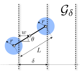
Figure 1: A Buffon “dumbbell” problem in 2-D.

For $r>0$, Eq.(34) shows that we must now consider the two neighboring $\ell_{2}$-balls of $\boldsymbol{p}$ and $\boldsymbol{q}$ in $P_{s^{\prime}}(\alpha,1|\phi)$ and estimate the probability that at least two points of these balls share the same dithered quantized projection onto $\hat{\boldsymbol{\varphi}}$. Following the same argument as above, this new problem is now equivalent to a new Buffon experiment if the previous needle is ended with two balls. In other words, we create a dumbbell shape formed by a segment of length $L$ on the extremities of which two balls of radius $r$ are centered (see Fig. 1).

It is then easy to see that $P_{s^{\prime}}(\alpha,1|\phi)$ is equivalent to the probability that there is no hyperplane of $\mathcal{G}_{\delta}$ intersecting only the part of the segment outside of the two balls when the dumbbell is thrown randomly in $\mathbb{R}^{N}$ as for previous Buffon’s needle. Otherwise, having such an intersection would mean that no pair of points (taken in distinct balls) lie in the same subvolume delimited by two consecutive hyperplanes, i.e., they do not have the same quantized projection, and conversely.

Let us parametrize this dumbbell by its distance $w\sim\mathcal{U}([0,\delta/2])$ (estimated from the middle of the segment) to the closest hyperplane $\mathcal{G}_{\delta}$ and by its orientation drawn uniformly at random in $\mathbb{S}^{N-1}$. By symmetry, only the angle $\theta\in[0,\pi]$ made by the dumbbell with the normal vector $\boldsymbol{e}_{1}$ to $\mathcal{G}_{\delta}$ is important in this parametrization [22]. Moreover, from Fig. 1, the absence of intersection amounts to imposing $w\geqslant\frac{1}{2}\,L|\cos\theta|-r$. The probability $P_{s^{\prime}}(\alpha,1|\phi)$ is thus obtained by

$$\textstyle P_{s^{\prime}}(\alpha,1|\phi) \textstyle=\int_{0}^{\pi}\kappa_{N}\,(\sin\theta)^{N-2}\,\mathrm{d}\theta\int_{0}^{\delta/2}\mathbb{I}(w\geqslant\tfrac{L}{2}|\cos\theta|-r)\tfrac{2}{\delta}\,\mathrm{d}w,$$

$$\textstyle=\tfrac{4\kappa_{N}}{\delta}\int_{0}^{\pi/2}(\sin\theta)^{N-2}\mathrm{d}\theta\int_{0}^{\delta/2}\mathbb{I}(w\geqslant\tfrac{L}{2}\cos\theta-r)\,\mathrm{d}w,$$

where $\kappa_{N}(\sin\theta)^{N-2}\mathrm{d}\theta$ is the area (normalized to the one of $\mathbb{S}^{N-1}$) of the thin spherical segment $\mathcal{S}_{\mathrm{d}\theta}(\theta):=\{\hat{\boldsymbol{v}}\in\mathbb{S}^{N-1}:\arccos(\boldsymbol{e}_{1}^{T}\hat{\boldsymbol{v}})\in[\theta,\theta+\mathrm{d}\theta]\}$, where $\kappa_{N}:=\frac{\Gamma(\frac{N}{2})}{\sqrt{\pi}\,\Gamma(\frac{N-1}{2})}=B(\frac{1}{2},\frac{N-1}{2})^{-1}$ and $B(k,l)=\Gamma(k)\Gamma(l)/\Gamma(k+l)$ is the Beta function.

It is important to remark that, from [22, 35],

$$\textstyle\ \tfrac{\sqrt{2}}{\sqrt{\pi}}\,(N+1)^{-\frac{1}{2}}\ \leqslant\ \tfrac{2\kappa_{N}}{N-1}\ \leqslant\ \tfrac{\sqrt{2}}{\sqrt{\pi}}\,(N-1)^{-\frac{1}{2}},$$ (35)

so that, for $N\geqslant 2$,

$$\tfrac{1}{\sqrt{2\pi}}\,(N+1)^{\frac{1}{2}}-1\ <\ \kappa_{N}\ \leqslant\ \tfrac{1}{\sqrt{2\pi}}\,(N-1)^{\frac{1}{2}}\quad\Rightarrow\ \kappa_{N}=\Theta(\sqrt{\tfrac{N}{2\pi}}).$$

Let us define two angles $0\leqslant\theta_{0}\leqslant\theta_{1}\leqslant\pi/2$ such that $\cos\theta_{0}=\min(\tfrac{\delta+2r}{L},1)$ and $\cos\theta_{1}=\tfrac{2r}{L}$, assuming $2r\leqslant L$ (otherwise, $P_{s^{\prime}}=1$). The angular integration domain can be split in three intervals: $[0,\theta_{0}]$, $[\theta_{0},\theta_{1}]$ and $[\theta_{1},\pi/2]$. Over the first interval, the integral is always zero since, either we have a zero measure interval ($\theta_{0}=0$) or $\mathbb{I}(w\geqslant\tfrac{L}{2}\cos\theta-r)=0$ since $\tfrac{L}{2}\cos\theta\geqslant\tfrac{L}{2}\cos\theta_{0}=\delta/2+r$ and $0\leqslant w\leqslant\delta/2$. Moreover, over the last interval $[\theta_{1},\pi/2]$, $I(w\geqslant\tfrac{L}{2}\cos\theta-r)=1$

Therefore, writing $a=L/\delta$,

$$\textstyle P_{s^{\prime}}(\alpha,1|\phi) \textstyle=\ \tfrac{4\kappa_{N}}{\delta}\int_{\theta_{0}}^{\theta_{1}}(\sin\theta)^{N-2}(\tfrac{\delta}{2}-\tfrac{L}{2}\cos\theta+r)\,\mathrm{d}\theta\ +\ 2\kappa_{N}\int_{\theta_{1}}^{\pi/2}(\sin\theta)^{N-2}\,\mathrm{d}\theta$$

$$\textstyle=1+\tfrac{4\kappa_{N}}{\delta}\int_{\theta_{0}}^{\theta_{1}}(\sin\theta)^{N-2}(\tfrac{\delta}{2}-\tfrac{L}{2}\cos\theta+r)\,\mathrm{d}\theta\ -\ 2\kappa_{N}\int_{0}^{\theta_{1}}(\sin\theta)^{N-2}\,\mathrm{d}\theta$$

$$\textstyle=1-\tfrac{4\kappa_{N}}{\delta}\int_{\theta_{0}}^{\theta_{1}}(\sin\theta)^{N-2}(\tfrac{L}{2}\cos\theta-r)\,\mathrm{d}\theta\ -\tfrac{4\kappa_{N}}{\delta}\int_{0}^{\theta_{0}}(\sin\theta)^{N-2}\,\tfrac{\delta}{2}\,\mathrm{d}\theta$$

$$\textstyle=1\ -\ \tfrac{4\kappa_{N}}{\delta}\int_{0}^{\theta_{1}}(\sin\theta)^{N-2}(\tfrac{L}{2}\cos\theta-r)\,\mathrm{d}\theta\ +\ \tfrac{4\kappa_{N}}{\delta}\int_{0}^{\theta_{0}}(\sin\theta)^{N-2}(\tfrac{L}{2}\cos\theta-(r+\tfrac{\delta}{2}))\,\mathrm{d}\theta$$

$$\textstyle=1\ -\ 2\kappa_{N}a\,\int_{0}^{1}(1-v^{2})^{\frac{N-3}{2}}\big{[}(v-\tfrac{2r}{L})_{+}-(v-\tfrac{2r+\delta}{L})_{+}\big{]}\mathrm{d}v,$$

applying a variable change $v=\cos\theta$ on the last line.

Let us study this last integral and the function $f(v)=(v-\tfrac{2r}{L})_{+}-(v-\tfrac{2r+\delta}{L})_{+}$. We can verify that $F(v):=\int_{0}^{v}f(v^{\prime})\mathrm{d}v^{\prime}$ is convex and reads

$$2F(v)\ =\ (v-\tfrac{2r}{L})^{2}_{+}-(v-\tfrac{2r+\delta}{L})^{2}_{+}\ =\ \begin{cases}0,&\text{if }v\leqslant\tfrac{2r}{L},\\ (v-\tfrac{2r}{L})^{2},&\text{if }\tfrac{2r}{L}<v\leqslant\tfrac{2r+\delta}{L},\\ \tfrac{\delta}{L}(2v-\tfrac{4r+\delta}{L}),&\text{if}\ v>\tfrac{2r+\delta}{L}.\end{cases}$$

Moreover, by integrating by part,

$$\textstyle\int_{0}^{1}(1-v^{2})^{\frac{N-3}{2}}f(v)\,\mathrm{d}v\ \textstyle=\int_{0}^{1}(N-3)\,v\,(1-v^{2})^{\frac{N-5}{2}}F(v)\,\mathrm{d}v,$$

The positive measure $\mu(v)=(N-3)\,v\,(1-v^{2})^{\frac{N-5}{2}}$ has unit mass over $[0,1]$ so that, by convexity of $F$ and using Jensen’s inequality,

$$\int_{0}^{1}F(v)\,\mu(v)\,\mathrm{d}v\ \geqslant\ F\big{(}\textstyle\int_{0}^{1}v\,\mu(v)\,\mathrm{d}v\big{)}.$$

However, since

$$\textstyle(N-3)\int_{0}^{1}(1-v^{2})^{\frac{N-5}{2}}\,v^{q}\,\mathrm{d}v=\ \textstyle\tfrac{N-3}{2}\,B(\tfrac{q+1}{2},\tfrac{N-3}{2})=\tfrac{\Gamma\big{(}\tfrac{q+1}{2}\big{)}\,\Gamma(\frac{N-1}{2})}{\Gamma\big{(}\tfrac{N+q-2}{2}\big{)}},$$ (36)

we find

$$\textstyle\textstyle\int_{0}^{1}v\,\mu(v)\,\mathrm{d}v=(N-3)\int_{0}^{1}(1-v^{2})^{\frac{N-5}{2}}\,v^{2}\,\mathrm{d}v\ =\tfrac{\sqrt{\pi}\,\Gamma(\frac{N-1}{2})}{2\,\Gamma(\frac{N}{2})}=\tfrac{1}{2\kappa_{N}},$$ (37)

and

$$P_{s^{\prime}}(\alpha,1|\phi)\ \leqslant\ 1-2\kappa_{N}a\,F({\textstyle\frac{1}{2\kappa_{N}}}).$$

From the definition of $F$ above, if ${\textstyle\frac{1}{2\kappa_{N}}}\leqslant\frac{2r}{L}$, $F=0$ and we cannot show anything. Let us thus set $2r=\tfrac{\lambda}{2\kappa_{N}}L$, where $\lambda\in(0,1)$ will be determined later. Notice that, since $s^{\prime}=\phi\,r$ and $\|\tilde{\boldsymbol{p}}-\tilde{\boldsymbol{q}}\|=\phi\,L$, we implicitly impose $2r/L=2s^{\prime}/\|\tilde{\boldsymbol{p}}-\tilde{\boldsymbol{q}}\|=\tfrac{\lambda}{2\kappa_{N}}$.

Then,

$$2F({\textstyle\frac{1}{2\kappa_{N}}})=\begin{cases}{\textstyle\frac{1}{4\kappa^{2}_{N}}}(1-\lambda)^{2},&\text{if }a\leqslant\tfrac{2\kappa_{N}}{1-\lambda},\\ {\textstyle\frac{1}{a}}(\tfrac{1}{\kappa_{N}}(1-\lambda)-{\textstyle\frac{1}{a}}),&\text{if }a\geqslant\tfrac{2\kappa_{N}}{1-\lambda},\end{cases}$$

so that, writing $\phi_{0}=\tfrac{2\kappa_{N}}{1-\lambda}$, we have

$$P_{s^{\prime}}(\alpha,1|\phi)\ \leqslant\ \begin{cases}1-\tfrac{a}{2\phi_{0}}(1-\lambda),&\text{if }a\leqslant\phi_{0},\\ \lambda+\tfrac{\phi_{0}}{2a}(1-\lambda),&\text{if }a\geqslant\phi_{0}.\end{cases}$$

Let us recall that $P_{s^{\prime}}(\alpha,1|\phi)$ is defined conditionally to $\phi=\|\boldsymbol{\varphi}\|$ with $\phi\sim\chi(N)$. Moreover, $a=\|\boldsymbol{p}-\boldsymbol{q}\|/\delta=\phi\|\tilde{\boldsymbol{p}}-\tilde{\boldsymbol{q}}\|/\delta=\alpha\phi$ with $\alpha=\|\tilde{\boldsymbol{p}}-\tilde{\boldsymbol{q}}\|/\delta$. Denoting the pdf of $\chi(N)$ by $\gamma_{N}(\phi)=c_{N}\phi^{N-1}\exp(-\tfrac{\phi^{2}}{2})$ and $c_{N}=2^{1-\frac{N}{2}}/\Gamma(\frac{N}{2})$, we can develop $P_{s^{\prime}}(\alpha,1)=\ \int_{0}^{+\infty}P_{s^{\prime}}(\alpha,1|\phi)\,\gamma_{N}(\phi)\ \mathrm{d}\phi$ as follows

$$P_{s^{\prime}}(\alpha,1) \textstyle\leqslant\ \int_{0}^{\phi_{0}/\alpha}(1-\tfrac{\alpha\phi}{2\phi_{0}}(1-\lambda))\,\gamma_{N}(\phi)\,\mathrm{d}\phi$$

$$\textstyle\quad+\ \int_{\phi_{0}/\alpha}^{+\infty}(\lambda+\tfrac{\phi_{0}}{2\alpha\phi}(1-\lambda))\,\gamma_{N}(\phi)\,\mathrm{d}\phi$$

$$\textstyle=\lambda\ +\ (1-\lambda)\int_{0}^{\phi_{0}/\alpha}(1-\tfrac{\alpha\phi}{2\phi_{0}})\,\gamma_{N}(\phi)\,\mathrm{d}\phi$$

$$\textstyle\qquad+\ (1-\lambda)\,\int_{\phi_{0}/\alpha}^{+\infty}\tfrac{\phi_{0}}{2\alpha\phi}\gamma_{N}(\phi)\,\mathrm{d}\phi$$

$$\textstyle=\lambda\ +\ (1-\lambda)\int_{0}^{+\infty}\varphi(\tfrac{\alpha\phi}{\phi_{0}})\,\gamma_{N}(\phi)\mathrm{d}\phi,$$

with $\varphi(t)=1-{\textstyle\frac{1}{2}}t$ if $0\leqslant t<1$ and $\varphi(t)={\textstyle\frac{1}{2t}}$ if $t\geqslant 1$.

We can notice that $t\varphi(t)$, which is equal to ${\textstyle\frac{1}{2}}t(2-t)$ over $[0,1]$ and to ${\textstyle\frac{1}{2}}$ for $t\geqslant 1$, is a concave function. Therefore, by Jensen inequality,

$$\textstyle\int_{0}^{+\infty}\varphi(\tfrac{\alpha\phi}{\phi_{0}})\,\gamma_{N}(\phi)\mathrm{d}\phi$$

$$\textstyle=\ \tfrac{c_{N}}{c_{N-1}}\,\int_{0}^{+\infty}\phi\,\varphi(\tfrac{\alpha\phi}{\phi_{0}})\,\gamma_{N-1}(\phi)\mathrm{d}\phi$$

$$\textstyle\leqslant\ \tfrac{c_{N}}{c_{N-1}}(\mathbb{E}_{\gamma_{N-1}}\phi)\,\varphi(\tfrac{\alpha\mathbb{E}_{\gamma_{N-1}}\phi}{\phi_{0}}).$$

We have also $c_{N}/c_{N-1}=\Gamma(\frac{N-1}{2})/(\sqrt{2}\Gamma(\frac{N}{2}))$ and $\mathbb{E}_{\gamma_{N-1}}\phi=\sqrt{2}\Gamma(\tfrac{N}{2})/\Gamma(\tfrac{N-1}{2})=\sqrt{2\pi}\kappa_{N}$, so that $\tfrac{c_{N}}{c_{N-1}}(\mathbb{E}_{\gamma_{N-1}}\phi)=1$ and

$$\tfrac{\alpha\mathbb{E}_{\gamma_{N-1}}\phi}{\phi_{0}}=\alpha\,\tfrac{1-\lambda}{2\kappa_{N}}\,\mathbb{E}_{\gamma_{N-1}}\phi=\sqrt{\tfrac{\pi}{2}}(1-\lambda)\alpha.$$

Consequently, since $\varphi(t)\leqslant\tfrac{2}{2+t}$,

$$P_{s^{\prime}}(\alpha,1) \textstyle\leqslant\lambda+(1-\lambda)\varphi\big{(}\sqrt{\tfrac{\pi}{2}}(1-\lambda)\alpha\big{)}$$

$$\textstyle\leqslant\lambda+(1-\lambda)\tfrac{2}{2+\sqrt{\frac{\pi}{2}}(1-\lambda)\alpha}$$

$$\textstyle=1-\tfrac{\sqrt{\frac{\pi}{2}}(1-\lambda)^{2}\alpha}{2+\sqrt{\frac{\pi}{2}}(1-\lambda)\alpha}=\ 1-\tfrac{\sqrt{\frac{2}{\pi}}\alpha}{2+\alpha}$$

$$\textstyle<\ 1-\tfrac{3\alpha}{8+4\alpha},$$

taking $(1-\lambda)=\sqrt{\tfrac{2}{\pi}}>3/4$.

Moreover, from the bounds on $\kappa_{N}$ given in (35), this shows also that

$$\tfrac{2s^{\prime}}{\|\tilde{\boldsymbol{p}}-\tilde{\boldsymbol{q}}\|}=\tfrac{2r}{L}=\tfrac{\lambda}{2\kappa_{N}}\geqslant(1-\sqrt{\tfrac{2}{\pi}})\sqrt{\tfrac{\pi}{2}}{\textstyle\frac{1}{(N-1)^{1/2}}}>\tfrac{1}{4\sqrt{N}},$$

as stated at the beginning of Lemma 1.

References

- [1] R. Baraniuk, M. Davenport, R. DeVore, and M. Wakin. A simple proof of the restricted isometry property for random matrices. Constructive Approximation, 28(3):253–263, 2008.
- [2] T. Blumensath and M. Davies. Iterative hard thresholding for compressive sensing. Appl. Comput. Harmon. Anal., 27(3):265–274, 2009.
- [3] P. T. Boufounos. Quantization and Erasures in Frame Representations. D.Sc. Thesis, MIT EECS, Cambridge, MA, January 2006.
- [4] P. T. Boufounos. Universal rate-efficient scalar quantization. IEEE Trans. Info. Theory, 58(3):1861–1872, March 2012.
- [5] P. T. Boufounos and R. G. Baraniuk. 1-bit compressive sensing. In Proc. Conf. Inform. Science and Systems (CISS), Princeton, NJ, March 19-21 2008.
- [6] P. T. Boufounos and S. Rane. Efficient coding of signal distances using universal quantized embeddings. In Proc. Data Compression Conference (DCC), Snowbird, UT, March 20-22 2013.
- [7] P. T. Boufounos, L. Jacques, F. Krahmer, and R. Saab. Quantization and compressive sensing. In book ”Compressed Sensing and its Applications”, Springer, 2014.
-
[8]
G. C. Buffon.
Essai d’arithmétique morale, volume 4 of Supplément
à l’histoire naturelle, 1777.
http://www.buffon.cnrs.fr. - [9] P. Bürgisser, F. Cucker, M. Lotz. Coverage processes on spheres and condition numbers for linear programming. The Annals of Probability, 38(2):570–604, 2010.
- [10] E. Candès, J. Romberg, and T. Tao. Stable signal recovery from incomplete and inaccurate measurements. Comm. Pure Appl. Math, 59(8):1207–1223, 2006.
- [11] E. J. Candes and T. Tao. Near-optimal signal recovery from random projections: Universal encoding strategies? Information Theory, IEEE Transactions on, 52(12):5406–5425, 2006.
- [12] S. S. Chen, D. L. Donoho, and M. A. Saunders. Atomic Decomposition by Basis Pursuit. SIAM Journal on Scientific Computing, 20(1):33–61, 1998.
- [13] W. Dai, H. V. Pham, and O. Milenkovic. Distortion-Rate Functions for Quantized Compressive Sensing. Technical Report arXiv:0901.0749, 2009.
- [14] V. K Goyal, M. Vetterli, and N. T. Thao. Quantized overcomplete expansions in : Analysis, synthesis, and algorithms. IEEE Trans. Info. Theory, 44(1):16–31, 1998.
- [15] V. K. Goyal, J. Kovačević, and J. A. Kelner. Quantized frame expansions with erasures. Applied and Computational Harmonic Analysis, 10(3):203–233, 2001.
- [16] V. K. Goyal, A. K. Fletcher, and S. Rangan. Compressive sampling and lossy compression. IEEE, Signal Processing Magazine, 25(2):48–56, 2008.
- [17] R.M. Gray and D.L. Neuhoff. Quantization. IEEE Trans. Info. Theory, 44(6):2325–2383, Oct 1998.
- [18] C. S. Güntürk, M. Lammers, A. M. Powell, R. Saab, and Ö. Yılmaz. Sobolev duals for random frames and quantization of compressed sensing measurements. Foundations of Computational Mathematics, 13(1):1–36, 2013.
- [19] J. D. Hey, T. M. Neugebauer, and C. M. Pasca. Georges-Louis Leclerc de Buffon’s ‘Essays on Moral Arithmetic’. In The Selten School of Behavioral Economics, pages 245–282. Springer, 2010.
- [20] L. Jacques, D. K. Hammond, and M. J. Fadili. Dequantizing Compressed Sensing: When Oversampling and Non-Gaussian Constraints Combine. IEEE Trans. Inf. Theory, 57(1):559–571, January 2011.
- [21] L. Jacques, D. K. Hammond, and M. J. Fadili. Stabilizing Nonuniformly Quantized Compressed Sensing With Scalar Companders. IEEE Trans. Inf. Theory, 59(12):7969 – 7984, January 2013.
- [22] L. Jacques. A Quantized Johnson Lindenstrauss Lemma: The Finding of Buffon’s Needle. IEEE Trans. Inf. Theory, 61(9):5012–5027, Sept. 2015.
- [23] L. Jacques, K. Degraux, and C. De Vleeschouwer. Quantized iterative hard thresholding: Bridging 1-bit and high-resolution quantized compressed sensing. In 10th international conference on Sampling Theory and Applications (SampTA 2013), arXiv:1305.1786, pages 105–108, Bremen, Germany, 2013.
- [24] L. Jacques, J. N. Laska, P. T. Boufounos, and R. G. Baraniuk. Robust 1-bit compressive sensing via binary stable embeddings of sparse vectors. IEEE Transactions on Information Theory, 59(4):2082–2102, 2013.
- [25] U. S. Kamilov, V. K. Goyal, S. Rangan. Message-passing de-quantization with applications to compressed sensing. Signal Processing, IEEE Transactions on, 60(12):6270–6281, 2012.
- [26] D. E. Knuth. Big omicron and big omega and big theta. ACM Sigact News, 8(2):18–24, 1976.
- [27] F. Krahmer, R. Saab, and R. Ward. Root-exponential accuracy for coarse quantization of finite frame expansions. IEEE Trans. Inform. Theory, 58(2):1069–1079, 2012.
- [28] B. K. Natarajan. Sparse approximate solutions to linear systems. SIAM journal on computing, 24(2):227–234, 1995.
- [29] H. Q. Nguyen, V.K. Goyal, and L.R. Varshney. Frame Permutation Quantization. Applied and Computational Harmonic Analysis (ACHA), Nov. 2010.
- [30] R. J. Pai. Nonadaptive lossy encoding of sparse signals Doctoral dissertation, Massachusetts Institute of Technology, 2006.
- [31] Y. Plan and R. Vershynin. Dimension reduction by random hyperplane tessellations. arXiv preprint arXiv:1111.4452, 2011.
- [32] Y. Plan and R. Vershynin. One-bit compressed sensing by linear programming. Communications on Pure and Applied Mathematics, 66(8):1275–1297, 2013.
- [33] A. M. Powell. Mean squared error bounds for the Rangan-Goyal soft thresholding algorithm. Appl. Comput. Harmon. Anal., 29:251–271, 2010.
- [34] A. M. Powell and J. T. Whitehouse. Error bounds for consistent reconstruction: Random polytopes and coverage processes. arXiv preprint arXiv:1405.7094, 2014.
- [35] F. Qi and Q.-M. Luo. Bounds for the ratio of two gamma functions–From Wendel’s and related inequalities to logarithmically completely monotonic functions. Banach J. Math. Anal, 6(2):132–158, 2012.
- [36] S. Rangan and V. K. Goyal. Recursive Consistent Estimation with Bounded Noise. IEEE Trans. Information Theory, 47:457–464, 2001.
- [37] N. T. Thao and M. Vetterli. Deterministic analysis of oversampled A/D conversion and decoding improvement based on consistent estimates. Signal Processing, IEEE Transactions on, 42(3): 519–531, 1994.
- [38] J. A. Tropp. Just relax: Convex programming methods for identifying sparse signals in noise. Information Theory, IEEE Transactions on, 52(3):1030–1051, 2006.