Turbulent diffusion of chemically reacting gaseous admixtures

Abstract

We study turbulent diffusion of chemically reacting gaseous admixtures in a developed turbulence. In our previous study [Phys. Rev. Lett. 80, 69 (1998)] using a path-integral approach for a delta-correlated in time random velocity field, we demonstrated a strong modification of turbulent transport in fluid flows with chemical reactions or phase transitions. In the present study we use the spectral tau approximation, that is valid for large Reynolds and Peclet numbers, and show that turbulent diffusion of the reacting species can be strongly depleted by a large factor that is the ratio of turbulent and chemical times (turbulent Damköhler number). We have demonstrated that the derived theoretical dependence of turbulent diffusion coefficient versus the turbulent Damköhler number is in a good agreement with that obtained previously in the numerical modelling of a reactive front propagating in a turbulent flow and described by the Kolmogorov-Petrovskii-Piskunov-Fisher equation. We have found that turbulent cross-effects, e.g., turbulent mutual diffusion of gaseous admixtures and turbulent Dufour-effect of the chemically reacting gaseous admixtures, are less sensitive to the values of stoichiometric coefficients. The mechanisms of the turbulent cross-effects are different from the molecular cross effects known in irreversible thermodynamics. In a fully developed turbulence and at large Peclet numbers the turbulent cross-effects are much larger than the molecular ones. The obtained results are applicable also to heterogeneous phase transitions.

I Introduction

Turbulent transport in flows with chemical reactions is of great interest in various applications, ranging from combustion to physics of turbulent atmosphere of the Earth (see, e.g., ZB85 ; F03 ; P04 ; EM11 ; SB11 ; SP06 ; PK97 ; W99 ; J05 ). During the decades turbulent transport of passive scalar and particles has been subject of an active research (see, e.g., handbooks MY75 ; CSA80 ; Mc90 ; ZRS90 ; BLA97 ; CST11 and reviews WA00 ; S03 ; BH03 ; KPE07 ; WA09 ; BE10 ). Many important problems, including particle clustering in isothermal EKR96a ; BF01 ; EKR02 ; FP04 ; EKR07 ; SA08 ; XB08 ; SSA08 and stratified EKR10 ; EKR13 turbulence, intermittency KR68 ; F95 , effective diffusion DF14 , the formation of large-scale inhomogeneous structures in spatial distribution of particles or different scalar fields in small-scale turbulence EKR96 ; EKR00 ; PM02 ; BEE04 ; RE05 ; EEKR06 ; SSEKR09 ; HKRB12 have been investigated in analytical, numerical and laboratory studies. However, impact of chemical reactions on turbulent transport have been studied mainly numerically and in the context of turbulent combustion (see, e.g., F03 ; P04 ; EM11 ; SB11 ).

Combustion process is the chemical reaction accompanied by heat release. Turbulent combustion can proceed as volume distributed chemical reaction (e.g., as a homogeneous burning of the turbulent premixed gaseous mixture) or propagate as a flame front in a turbulent flow separating fresh unburned fuel and combustion products (see, e.g., D08 ). In both cases turbulence is created by an external forcing and can be enhanced by intrinsic instability of the flame front (see, e.g., ZB85 ; P04 ; VV02 ; HT04 ).

Notice that temperature and equilibrium composition of combustion products are purely thermodynamic characteristics determined by the thermodynamic equilibrium laws which yield a relation between the initial and final stages. In this case chemical kinetics described by a one-step Arrhenius model provides results which usually are in a good agreement with experimental data. On the contrary, in order to reproduce transient processes that are accompanied by compression and shock waves, it is necessary to take into account the detailed chemical reaction mechanisms involving several hundreds chemical reactions. This complex chemistry determines the chemical time scales, such as induction time and period of exothermal reaction, competing with transport time scales in formation of the zone of energy release. The latter determines the evolution of the propagating flame (see, e.g., ML14 ).

In a turbulent atmosphere the most common are the volume distributed chemical reactions, while during wild fires propagation of the turbulent flame front is of particular interest in the atmospheric and industrial applications (see, e.g., SP06 ; PK97 ; W99 ; J05 ). In the previous studies the main attention was focused on evaluation of nonlinear sources in the governing equations for concentrations of chemical species. In such description the effect of chemical reactions on turbulent transport coefficients has been neglected. For the first time the effect of chemistry on turbulent diffusion was studied in EKR98 by means of a path-integral approach for the Kraichnan-Kazantsev model (see KR68 ; K68 ) of the random velocity field, and it was found that turbulent diffusion can be strongly depleted by chemical reactions or phase transitions. It was also shown in EKR98 that there exists an additional non-diffusive turbulent flux of number density of gaseous admixture (proportional to the mean temperature gradient multiplied by the number density of gaseous admixture) and additional turbulent heat flux (proportional to the gradient of the mean number density of gaseous admixture) in flows with chemical reactions or phase transitions.

The effect of chemistry on turbulent diffusion has been recently studied in BH11 using mean-field simulations (MFS) and direct numerical simulations (DNS). In these simulations a reactive front propagation in a turbulent flow was investigated using the Kolmogorov-Petrovskii- Piskunov (KPP) equation KPP37 or the Fisher equation F37 . This equation has also been amended by an advection term to describe the interaction with a turbulent velocity field BN09 ; PBN10 . In MFS of BH11 memory effects of turbulent diffusion have been taken into account to determine the front speed in the case when the turbulent time, $\tau_{0}$, is much larger than the characteristic chemical time, $\tau_{c}$. It was found that the memory effects saturate the front speed to values of the turbulent speed, while the nonlinearity of the reaction term increases the front speed. This study allows to determine the dependence of the turbulent diffusion coefficient versus the turbulent Damköhler number, ${\rm Da}_{{}_{\rm T}}=\tau_{0}/\tau_{c}$.

In the present study we investigate turbulent transport of chemically reacting gaseous admixtures in a developed turbulence using a spectral tau approach (high-order closure procedure), see, e.g., O70 ; PFL76 ; Mc90 . We have demonstrated here the existence of the turbulent cross-effects, including turbulent mutual diffusion of gaseous admixtures and turbulent Dufour-effect. The mechanisms of these cross-effects are different from the molecular cross effects known in irreversible thermodynamics (see, e.g., GM84 ). In a developed turbulence and at large Peclet numbers the turbulent cross-effects are much larger than the molecular ones. These results are also valid for heterogeneous phase transitions. We show that for a large turbulent Damköhler number ${\rm Da}_{{}_{\rm T}}\gg 1$ turbulent diffusion of the admixtures can be strongly reduced by a large factor ${\rm Da}_{{}_{\rm T}}$ depending on the value of stoichiometric coefficients of chemical species. In this paper we illustrate effect of chemistry on turbulent diffusion using simple global one step chemical reactions taking into account the reaction order. Such approach provides qualitatively and often quantitatively correct physics.

The paper is organized as follows. The governing equations and applied methods are formulated in Section II. Turbulent fluxes of chemically reacting admixtures are determined in Sections III and IV. Comparison of theoretical predictions with numerical simulations is given in Section V. Finally, in Section VI we draw conclusions and discuss the implications of the obtained results.

II Governing equations

Advection-diffusion equation for the number density $n_{\beta}(t,{\bm{x}})$ of chemically reactive admixtures in a turbulent flow reads:

$$\frac{\partial n_{\beta}}{\partial t}+{\bm{\nabla}\cdot}(n_{\beta}\,{\bm{v}})=-\nu_{\beta}\hat{W}(n_{\beta},T)+\hat{D}(n_{\beta}),$$ (1)

where ${\bm{v}}(t,{\bm{x}})$ is the instantaneous fluid velocity field, $\hat{D}(n_{\beta})=$ div $[\rho\,D_{\beta}{\bm{\nabla}}(n_{\beta}/\rho)]$ is the linear diffusion operator of $n_{\beta}$ (see, e. g., LL87 ), $D_{\beta}$ is the coefficient of the molecular diffusion based on molecular Fick’s law, $T$ is the fluid temperature, $-\nu_{\beta}\hat{W}(n_{\beta},T)$ is the source (or sink) term and $\nu_{\beta}$ is the stoichiometric coefficient that is the order of the reaction with respect to species $\beta$, $\sum_{\beta=1}^{m}\,\nu_{\beta}$ is the overall order of the reaction and $m$ is total number of species. The function $\hat{W}(n_{\beta},T)$ satisfies to the Arrhenius law (see, e.g., ML08 ):

$$\hat{W}=A\exp\left(-E_{a}/R\,T\right)\,\Large{\Pi}_{\beta=1}^{m}\,(n_{\beta})^{\nu_{\beta}},$$ (2)

where $A$ is the reaction rate constant, $E_{a}$ is the activation energy and $R$ is the universal gas constant. Evolution of the temperature field $T(t,{\bm{x}})$ in a turbulent fluid flow is determined by the following equation

$${\partial T\over\partial t} + ({\bm{v}}\cdot{\bm{\nabla}})T+(\gamma-1)T({\bm{\nabla}}\cdot{\bm{v}})$$ (3)

$$=q\hat{W}(n_{\beta},T)+\hat{D}(T),$$

where the term $\hat{D}(T)=\rho^{-1}$   div $[\rho\,\chi{\bm{\nabla}}T]$ determines the molecular diffusion of the fluid temperature, $\chi$ is the coefficient of molecular diffusion of temperature, $q=Q/\rho c_{p}$, $Q$ is the reaction energy release, $c_{p}$ is the specific heat at constant pressure, $\rho$ is the fluid density and $\gamma=c_{p}/c_{v}$ is the ratio of specific heats. The density $\rho$ and the velocity ${\bm{v}}$ of the fluid satisfy the continuity equation

$${\partial\rho\over\partial t}+{\bm{\nabla}}\cdot(\rho{\bm{v}})=0,$$ (4)

and the Navier-Stokes equation:

$${\partial{\bm{v}}\over\partial t} + ({\bm{v}}\cdot{\bm{\nabla}}){\bm{v}}=-{1\over\rho}{\bm{\nabla}}P+\hat{D}_{\nu}({\bm{v}}),$$ (5)

and $\hat{D}_{\nu}({\bm{v}})$ is the viscous term and $P$ is the fluid pressure.

To study the formation of large-scale inhomogeneous structures, Eqs. (1) and (3) are averaged over an ensemble of turbulent velocity fields. Using a mean-field approach, we decompose $n_{\beta}$ and $T$ into the mean quantities, $\overline{N}_{\beta}$ and $\overline{T}$, and fluctuations $n^{\prime}_{\beta}$ and $\theta$, where $\overline{n^{\prime}_{\beta}}=0$ and $\overline{\theta}=0$. We decompose the velocity field in a similar fashion, and assume for simplicity vanishing mean fluid velocity, $\overline{\bm{U}}=0$. Averaging Eqs. (1) and (3) over an ensemble of turbulent velocity fields we obtain the equations for the mean fields:

$$\frac{\partial\overline{N}_{\beta}}{\partial t} + {\bm{\nabla}\cdot}\langle n^{\prime}_{\beta}\,{\bm{u}}\rangle=-\nu_{\beta}\overline{W}+\hat{D}(\overline{N}_{\beta}),$$ (6)

$$\frac{\partial\overline{T}}{\partial t} + {\bm{\nabla}\cdot}\langle\theta\,{\bm{u}}\rangle+(\gamma-2)\langle\theta({\bm{\nabla}}\cdot{\bm{u}})\rangle$$ (7)

$$=q\overline{W}+\hat{D}(\overline{T}),$$

where ${\bm{u}}$ are the fluid velocity fluctuations, $\overline{W}\equiv\langle\hat{W}(n_{\beta},T)\rangle$ and angular brackets imply the averaging over the statistics of turbulent velocity field. To obtain a closed system of the mean-field equations one needs to determine the turbulent fluxes $\langle n^{\prime}_{\beta}\,{\bm{u}}\rangle$ and $\langle\theta\,{\bm{u}}\rangle$ as well as $\langle\theta({\bm{\nabla}}\cdot{\bm{u}})\rangle$. To this end we use the following equations for fluctuations $n^{\prime}_{\beta}=n_{\beta}-\overline{N}_{\beta}$ and $\theta=T-\overline{T}$:

$$\frac{\partial n^{\prime}_{\beta}}{\partial t}+{\bm{\nabla}\cdot}\Big{(}n^{\prime}_{\beta}\,{\bm{u}}-\langle n^{\prime}_{\beta}\,{\bm{u}}\rangle\Big{)}=-\nu_{\beta}\Big{(}\hat{W}-\overline{W}\Big{)}$$

$$\quad-{\bm{\nabla}\cdot}(\overline{N}_{\beta}\,{\bm{u}})+\hat{D}(n^{\prime}_{\beta}),$$ (8)

$$\frac{\partial\theta}{\partial t}+{\bm{\nabla}\cdot}\Big{(}\theta\,{\bm{u}}-\langle\theta\,{\bm{u}}\rangle\Big{)}+(\gamma-2)\Big{[}\theta({\bm{\nabla}}\cdot{\bm{u}})-\langle\theta({\bm{\nabla}}\cdot{\bm{u}})\rangle\Big{]}$$

$$\quad=q\left[\hat{W}-\overline{W}\right]-({\bm{u}}\cdot{\bm{\nabla}})\overline{T}-(\gamma-1)\overline{T}({\bm{\nabla}}\cdot{\bm{u}})+\hat{D}(\theta).$$

(9)

These equations are obtained by subtracting Eqs. (6) and (7) for the mean fields from Eqs. (1) and (3) for the total fields.

Now we assume that the temperature fluctuations are much smaller than the mean temperature, and the fluctuations of the number density of admixtures are much smaller than mean values. This allows us to expand the source term in a series:

$$\hat{W}-\overline{W} = \sum_{\beta=1}^{m}\left({\partial\hat{W}\over\partial n_{\beta}}\right)_{\overline{N}_{\beta}}n^{\prime}_{\beta}+\left({\partial\hat{W}\over\partial T}\right)_{\overline{T}}\theta$$ (10)

$$+ O\left[(n^{\prime}_{\beta})^{2};\theta^{2};n^{\prime}_{\beta}\,\theta\right]\equiv\overline{W}(C^{\prime}_{n}+C^{\prime}_{T}),$$

where we take into account that for the Arheneus law (2):

$$\left({\partial\ln\hat{W}\over\partial n_{\beta}}\right)_{\overline{N}_{\beta}}={\nu_{\beta}\over\overline{N}_{\beta}},\quad\left({\partial\ln\hat{W}\over\partial T}\right)_{\overline{T}}={E_{a}\over R\overline{T}^{2}}.$$ (11)

Here we introduced the following new variables:

$$C^{\prime}_{n} = \sum_{\beta=1}^{m}{\nu_{\beta}\over\overline{N}_{\beta}}n^{\prime}_{\beta},\quad C^{\prime}_{T}={E_{a}\over R\overline{T}^{2}}\theta,$$ (12)

where the evolutionary equations for $C^{\prime}_{n}$ and $C^{\prime}_{T}$ read:

$$\frac{\partial C^{\prime}_{n}}{\partial t}+{\bm{\nabla}\cdot}\Big{(}C^{\prime}_{n}\,{\bm{u}}-\langle C^{\prime}_{n}\,{\bm{u}}\rangle\Big{)}=-\alpha_{n}\overline{W}(C^{\prime}_{n}+C^{\prime}_{T})$$

$$\quad-\sum_{\beta=1}^{m}{\nu_{\beta}\over\overline{N}_{\beta}}{\bm{\nabla}\cdot}(\overline{N}_{\beta}\,{\bm{u}})+\hat{D}(C^{\prime}_{n}),$$ (13)

$$\frac{\partial C^{\prime}_{T}}{\partial t}+{\bm{\nabla}\cdot}\Big{(}C^{\prime}_{T}\,{\bm{u}}-\langle C^{\prime}_{T}\,{\bm{u}}\rangle\Big{)}+(\gamma-2)\Big{[}C^{\prime}_{T}({\bm{\nabla}}\cdot{\bm{u}})$$

$$\quad-\langle C^{\prime}_{T}({\bm{\nabla}}\cdot{\bm{u}})\rangle\Big{]}=\alpha_{{}_{T}}\overline{W}(C^{\prime}_{n}+C^{\prime}_{T})+\hat{D}(C^{\prime}_{T})$$

$$\quad-{\alpha_{{}_{T}}\over q}\,\left[({\bm{u}}\cdot{\bm{\nabla}})\overline{T}+(\gamma-1)\overline{T}({\bm{\nabla}}\cdot{\bm{u}})\right],$$ (14)

where

$$\alpha_{n} = \sum_{\beta=1}^{m}{\nu_{\beta}\over\overline{N}_{\beta}},\quad\alpha_{{}_{T}}={qE_{a}\over R\overline{T}^{2}}.$$ (15)

Using Eqs. (13)-(14) and the Navier-Stokes equation (5) we derive equations for the second-order moments $\langle C^{\prime}_{n}\,{\bm{u}}\rangle$ and $\langle C^{\prime}_{T}\,{\bm{u}}\rangle$:

$$\frac{\partial\langle C^{\prime}_{n}\,u_{i}\rangle}{\partial t}=-\alpha_{n}\overline{W}\Big{(}\langle C^{\prime}_{n}\,u_{i}\rangle+\langle C^{\prime}_{T}\,u_{i}\rangle\Big{)}+\hat{\cal N}\langle C^{\prime}_{n}\,u_{i}\rangle$$

$$\quad-\sum_{\beta=1}^{m}\nu_{\beta}\Big{[}\langle u_{i}\,u_{j}\rangle\,\nabla_{j}\ln\overline{N}_{\beta}+\langle u_{i}({\bm{\nabla}}\cdot{\bm{u}})\rangle\Big{]},$$ (16)

$$\frac{\partial\langle C^{\prime}_{T}\,u_{i}\rangle}{\partial t}={\alpha_{{}_{T}}\over q}\,\Big{[}q\overline{W}\left(\langle C^{\prime}_{n}\,u_{i}\rangle+\langle C^{\prime}_{T}\,u_{i}\rangle\right)-\langle u_{i}\,u_{j}\rangle\,\nabla_{j}\overline{T}$$

$$\quad-(\gamma-1)\overline{T}\,\langle u_{i}({\bm{\nabla}}\cdot{\bm{u}})\rangle\Big{]}+\hat{\cal N}\langle C^{\prime}_{T}\,u_{i}\rangle,$$ (17)

where $\hat{\cal N}\langle C^{\prime}_{n}\,u_{i}\rangle$ and $\hat{\cal N}\langle C^{\prime}_{T}\,u_{i}\rangle$ include the third-order moments caused by the nonlinear terms and the second-order moments due to the molecular dissipative terms:

$$\hat{\cal N}\langle C^{\prime}_{n}\,u_{i}\rangle=-\langle[{\bm{\nabla}\cdot}(C^{\prime}_{n}\,{\bm{u}})]\,u_{i}\rangle+\langle\hat{D}(C^{\prime}_{n})\,u_{i}\rangle$$

$$\quad-\langle C^{\prime}_{n}\,[({\bm{u}}\cdot{\bm{\nabla}})u_{i}+\rho^{-1}\nabla_{i}p^{\prime}]\rangle+\langle C^{\prime}_{n}\,\hat{D}_{\nu}(u_{i})\rangle,$$ (18)

$$\hat{\cal N}\langle C^{\prime}_{T}\,u_{i}\rangle=-\langle[{\bm{\nabla}\cdot}(C^{\prime}_{T}\,{\bm{u}})+(\gamma-2)C^{\prime}_{T}({\bm{\nabla}}\cdot{\bm{u}})]\,u_{i}\rangle$$

$$\quad+\langle\hat{D}(C^{\prime}_{T})\,u_{i}\rangle-\langle C^{\prime}_{T}\,[({\bm{u}}\cdot{\bm{\nabla}})u_{i}+\rho^{-1}\nabla_{i}p^{\prime}]\rangle$$

$$\quad+\langle C^{\prime}_{n}\,\hat{D}_{\nu}(u_{i})\rangle,$$ (19)

and $p^{\prime}$ are the fluid pressure fluctuations.

In the anelastic approximation for the low- Mach-number flows (Ma $=u/c_{s}\ll 1)$ and for hydrodynamic times that are much larger than the acoustic times, the continuity equation for surrounding fluid reads ${\bm{\nabla}}\cdot{\bm{u}}=-({\bm{u}}\cdot{\bm{\nabla}})\ln\rho$. We consider the ideal gases. Therefore,

$$\overline{T}\,\langle u_{i}({\bm{\nabla}}\cdot{\bm{u}})\rangle=\langle u_{i}\,u_{j}\rangle\,(\nabla_{j}\ln\overline{P}-\nabla_{j}\ln\overline{P}).$$ (20)

In a particular case when there is no external pressure gradient, ${\bm{\nabla}}\overline{P}=0$, (e.g., there is no mean flow), Eq. (20) yields:

$$\overline{T}\,\langle u_{i}({\bm{\nabla}}\cdot{\bm{u}})\rangle=\langle u_{i}\,u_{j}\rangle\,\nabla_{j}\overline{T},$$ (21)

where $\overline{P}$ is the mean fluid pressure. This allows us to rewrite Eqs. (16)-(17) in the following form:

$$\frac{\partial\langle C^{\prime}_{n}\,u_{i}\rangle}{\partial t}=-\alpha_{n}\overline{W}\Big{(}\langle C^{\prime}_{n}\,u_{i}\rangle+\langle C^{\prime}_{T}\,u_{i}\rangle\Big{)}+\hat{\cal N}\langle C^{\prime}_{n}\,u_{i}\rangle$$

$$\quad-\langle u_{i}\,u_{j}\rangle\,\nabla_{j}\sum_{\beta=1}^{m}\nu_{\beta}\Big{[}\ln\overline{N}_{\beta}+\ln\overline{T}\Big{]},$$ (22)

$$\frac{\partial\langle C^{\prime}_{T}\,u_{i}\rangle}{\partial t}=\alpha_{{}_{T}}\Big{[}\overline{W}\left(\langle C^{\prime}_{n}\,u_{i}\rangle+\langle C^{\prime}_{T}\,u_{i}\rangle\right)-{\gamma\over q}\,\langle u_{i}\,u_{j}\rangle\,\nabla_{j}\overline{T}\Big{]}$$

$$\quad+\hat{\cal N}\langle C^{\prime}_{T}\,u_{i}\rangle.$$ (23)

Now we introduce a new variable $C^{\prime}=C^{\prime}_{n}+C^{\prime}_{T}$. Equations (13)-(14) allow us to derive equation for the second-order moment $\langle C^{\prime}\,u_{i}\rangle$:

$$\frac{\partial\langle C^{\prime}\,u_{i}\rangle}{\partial t}=-\tau_{c}^{-1}\,\langle C^{\prime}\,u_{i}\rangle+\hat{\cal N}\langle C^{\prime}\,u_{i}\rangle-\langle u_{i}\,u_{j}\rangle$$

$$\,\times\Big{[}\sum_{\beta=1}^{m}\nu_{\beta}\,\nabla_{j}\Big{(}\ln\overline{N}_{\beta}+\ln\overline{T}\Big{)}+{\gamma\over q}\,\alpha_{{}_{T}}\,\nabla_{j}\overline{T}\Big{]},$$ (24)

where $\tau_{c}^{-1}=\overline{W}(\alpha_{n}-\alpha_{{}_{T}})$ is the inverse chemical time, $\hat{\cal N}\langle C^{\prime}\,u_{i}\rangle=\hat{\cal N}\langle C^{\prime}_{n}\,u_{i}\rangle+\hat{\cal N}\langle C^{\prime}_{T}\,u_{i}\rangle$ and the third-order moments $\hat{\cal N}\langle C^{\prime}_{n}\,u_{i}\rangle$ and $\hat{\cal N}\langle C^{\prime}_{T}\,u_{i}\rangle$ are determined by Eqs. (18)-(19).

It should be noted that the anelastic approximation is used in the continuity equation for the surrounding fluid. The chemical time appears only in the equation for the number density for species and the temperature equation. Since the ratio of spatial density of species is assumed to be much smaller than the density of the surrounding fluid (i.e., small mass-loading parameter), there is only one-way coupling, i.e., no effect of species on the fluid flow. Due to the same reason the energy release (or absorbtion of energy) caused by chemical reactions is much smaller than the internal energy of the surrounding fluid. This implies that even small chemical time does not affect the fluid characteristics.

III Turbulent flux of $C$

The equation for the second-order moment (24) includes the first-order spatial differential operators applied to the third-order moments $\hat{\cal N}F^{(III)}$ [see Eqs. (18)-(19)]. To close the system of equations it is necessary to express the third-order terms $\hat{\cal N}F^{(III)}$ through the lower-order moments $F^{(II)}$ (see, e.g., O70 ; MY75 ; Mc90 ). We use the spectral $\tau$ approximation which postulates that the deviations of the third-order moments, $\hat{\cal N}F^{(III)}({\bm{k}})$, from the contributions to these terms afforded by the background turbulence, $\hat{\cal N}F^{(III,0)}({\bm{k}})$, can be expressed through the similar deviations of the second-order moments, $F^{(II)}({\bm{k}})-F^{(II,0)}({\bm{k}})$:

$$\hat{\cal N}F^{(III)}({\bm{k}})-\hat{\cal N}F^{(III,0)}({\bm{k}})$$

$$\quad\quad\quad=-{1\over\tau_{r}(k)}\,\Big{[}F^{(II)}({\bm{k}})-F^{(II,0)}({\bm{k}})\Big{]},$$ (25)

(see, e.g., O70 ; PFL76 ; RK07 ), where $\tau_{r}(k)$ is the scale-dependent relaxation time, which can be identified with the correlation time $\tau(k)$ of the turbulent velocity field for large Reynolds and Peclet numbers. The functions with the superscript $(0)$ correspond to the background turbulence with zero gradients of the mean temperature, the mean number density and the mean fluid density.

In order to elucidate the spectral $\tau$ approach in the following we present the explicit form of terms in Eq. (25) corresponding to the second-order moments, $F^{(II)}({\bf k})\equiv\langle C^{\prime}_{n}({\bm{k}})\,u_{i}(-{\bm{k}})\rangle$, and the third-order moments $\hat{\cal N}F^{(III)}({\bm{k}})\equiv\hat{\cal N}\langle C^{\prime}_{n}\,u_{i}\rangle_{\bm{k}}$:

$$\hat{\cal N}\langle C^{\prime}_{n}\,u_{i}\rangle_{\bm{k}}-\hat{\cal N}\langle C^{\prime}_{n}\,u_{i}\rangle_{\bm{k}}^{(0)}$$

$$\quad=-{1\over\tau(k)}\,\Big{[}\langle C^{\prime}_{n}({\bm{k}})\,u_{i}(-{\bm{k}})\rangle-\langle C^{\prime}_{n}({\bm{k}})\,u_{i}(-{\bm{k}})\rangle^{(0)}\Big{]}.$$

(26)

Similarly one can formulate Eq. (25) for all other third-order and second-order correlators involving velocity, temperature and species number density fluctuations in ${\bf k}$-space. Validation of the $\tau$ approximation for different situations has been performed in numerous numerical simulations and analytical studies (see, e.g., review BS05 ; and also discussion in RK07 , Sec. 6).

The $\tau$-approximation is in general similar to Eddy Damped Quasi Normal Markowian (EDQNM) approximation. However some principle difference exists between these two approaches (see O70 ; Mc90 ). The EDQNM closures do not relax to equilibrium, and this procedure does not describe properly the motions in the equilibrium state in contrast to the $\tau$-approximation. Within the EDQNM theory, there is no dynamically determined relaxation time, and no slightly perturbed steady state can be approached O70 . In the $\tau$-approximation, the relaxation time for small departures from equilibrium is determined by the random motions in the equilibrium state, but not by the departure from equilibrium. We use the $\tau$-approximation, but not the EDQNM approximation because we consider a case when the characteristic scales of variations of the mean number density of admixtures and the mean temperature are much larger than the integral turbulence scale. Analysis performed in O70 showed that the $\tau$-approximation describes the relaxation to equilibrium state significantly more accurately than the EDQNM approach.

The $\tau$ approach is an universal tool in turbulent transport that allows to obtain closed results and compare them with the results of laboratory experiments, observations and numerical simulations. The $\tau$ approximation reproduces many well-known phenomena found by other methods in turbulent transport of particles and magnetic fields, in turbulent convection and stably stratified turbulent flows BS05 ; RK07 ; RKKB11 .

Note that when the gradients of the mean temperature and the mean number density are zero, the turbulent heat flux and the turbulent flux of chemical admixtures vanish, and the contributions of the corresponding fluctuations [the terms with the superscript (0)], vanish as well. Consequently, Eq. (26) reduces to $\hat{\cal N}\langle C^{\prime}_{n}\,u_{i}\rangle_{\bm{k}}=-\langle C^{\prime}_{n}({\bm{k}})\,u_{i}(-{\bm{k}})\rangle/\tau(k)$. We also assume that the characteristic time of variation of the second-order moments are substantially larger than the correlation time $\tau(k)$ for all turbulence scales. Therefore, the steady-state version of Eq. (24), written in the Fourier space yields the following formulae for the turbulent flux $\langle C^{\prime}({\bm{k}})\,u_{i}(-{\bm{k}})\rangle$:

$$\langle C^{\prime}({\bm{k}})\,u_{i}(-{\bm{k}})\rangle=-\tau_{\rm eff}(k)\,\langle u_{i}({\bm{k}})\,u_{j}(-{\bm{k}})\rangle\,$$

$$\quad\quad\times\Big{[}\sum_{\beta=1}^{m}\nu_{\beta}\,\nabla_{j}\Big{(}\ln\overline{N}_{\beta}+\ln\overline{T}\Big{)}+{\gamma\over q}\,\alpha_{{}_{T}}\,\nabla_{j}\overline{T}\Big{]},$$ (27)

where $\tau^{-1}_{\rm eff}(k)=\tau^{-1}_{c}+\tau^{-1}(k)$.

To integrate in ${\bm{k}}$-space we need to choose a model of the background turbulence. In order to separate the turbulent transport effects caused by the chemistry from those caused by inhomogeneity of turbulence we consider isotropic and homogeneous background turbulence, $\langle u_{i}({\bm{k}})\,u_{j}(-{\bm{k}})\rangle$ (see, e.g., B53 ):

$$\langle u_{i}({\bm{k}})\,u_{j}(-{\bm{k}})\rangle={u_{0}^{2}\,E_{T}(k)\over 8\pi k^{2}}\Big{[}\delta_{ij}-{k_{i}\,k_{j}\over k^{2}}\Big{]},$$ (28)

where $E_{T}(k)=(\mu-1)k_{0}^{-1}(k/k_{0})^{-\mu}$ is the energy spectrum function with the exponent $1<\mu<3$, $\tau(k)=2\,\tau_{0}\,(k/k_{0})^{1-\mu}$ is the turbulent correlation time, $\tau_{0}=\ell/u_{0}$ is the characteristic turbulent time and $u_{0}$ is the characteristic turbulent velocity in the integral scale $\ell$.

After integration in ${\bm{k}}$ space we obtain the turbulent flux $\langle C^{\prime}\,u_{i}\rangle=\int\langle C^{\prime}({\bm{k}})\,u_{i}(-{\bm{k}})\rangle\,d{\bm{k}}$:

$$\langle C^{\prime}\,u_{i}\rangle = -D^{T}_{C}\,\Big{[}\sum_{\beta=1}^{m}\nu_{\beta}\,\nabla_{j}\Big{(}\ln\overline{N}_{\beta}+\ln\overline{T}\Big{)}$$ (29)

$$+{\gamma\over q}\,\alpha_{{}_{T}}\,\nabla_{j}\overline{T}\Big{]},$$

where $D^{T}_{0}=\tau_{0}u_{0}^{2}/3$, and the turbulent diffusion coefficient reads:

$$D^{T}_{C}=D^{T}_{0}\,\left(1-{\ln(1+2{\rm Da}_{{}_{\rm T}})\over 2{\rm Da}_{{}_{\rm T}}}\right),$$ (30)

where ${\rm Da}_{{}_{\rm T}}=\tau_{0}/\tau_{c}$ is the turbulent Damköhler number. Here we used that $\int\tau_{\rm eff}(k)\langle u_{i}({\bm{k}})\,u_{j}(-{\bm{k}})\rangle\,d{\bm{k}}=D^{T}_{C}\delta_{ij}$. The asymptotic behaviour of the turbulent diffusion coefficient is as follows: when ${\rm Da}_{{}_{\rm T}}\ll 1$, the turbulent diffusion coefficient is

$$D^{T}_{C}=D^{T}_{0}\,{\rm Da}_{{}_{\rm T}}\left(1-{4{\rm Da}_{{}_{\rm T}}\over 3}\right),$$ (31)

while for ${\rm Da}_{{}_{\rm T}}\gg 1$, it is

$$D^{T}_{C}=D^{T}_{0}\,\left(1-{\ln{\rm Da}_{{}_{\rm T}}\over 2{\rm Da}_{{}_{\rm T}}}\right).$$ (32)

Equations (27) and (29)-(32) allow us to determine the turbulent transport coefficients for gaseous admixtures and temperature field (see next section).

IV Turbulent transport of admixtures and temperature

Using Eqs. (10)-(11) we rewrite Eqs. (8)-(9) for the fluctuations of the number density of admixtures, $n^{\prime}_{\beta}=n_{\beta}-\overline{N}_{\beta}$, and the fluid temperature field, $\theta=T-\overline{T}$, in the following form:

$$\frac{\partial n^{\prime}_{\beta}}{\partial t}+{\bm{\nabla}\cdot}\Big{(}n^{\prime}_{\beta}\,{\bm{u}}-\langle n^{\prime}_{\beta}\,{\bm{u}}\rangle\Big{)}=-\nu_{\beta}\overline{W}(C^{\prime}_{n}+C^{\prime}_{T})$$

$$\quad-{\bm{\nabla}\cdot}(\overline{N}_{\beta}\,{\bm{u}})+\hat{D}(n^{\prime}_{\beta}),$$ (33)

$$\frac{\partial\theta}{\partial t}+{\bm{\nabla}\cdot}\Big{(}\theta\,{\bm{u}}-\langle\theta\,{\bm{u}}\rangle\Big{)}+(\gamma-2)\Big{[}\theta({\bm{\nabla}}\cdot{\bm{u}})-\langle\theta({\bm{\nabla}}\cdot{\bm{u}})\rangle\Big{]}$$

$$\quad=q\overline{W}(C^{\prime}_{n}+C^{\prime}_{T})-({\bm{u}}\cdot{\bm{\nabla}})\overline{T}-(\gamma-1)\overline{T}({\bm{\nabla}}\cdot{\bm{u}})$$

$$\quad+\hat{D}(\theta).$$ (34)

To close a system of the mean-field equations we determine the turbulent fluxes $\langle n^{\prime}_{\beta}\,{\bm{u}}\rangle$ and $\langle\theta\,{\bm{u}}\rangle$. Equations for these second moments read:

$$\frac{\partial\langle n^{\prime}_{\beta}\,u_{i}\rangle}{\partial t} = -\nu_{\beta}\overline{W}\langle C^{\prime}\,u_{i}\rangle-\langle u_{i}\,u_{j}\rangle\,\nabla_{j}\overline{N}_{\beta}$$ (35)

$$-\overline{N}_{\beta}\,\langle u_{i}({\bm{\nabla}}\cdot{\bm{u}})\rangle+\hat{\cal N}\langle n^{\prime}_{\beta}\,u_{i}\rangle,$$

$$\frac{\partial\langle\theta\,u_{i}\rangle}{\partial t} = q\overline{W}\langle C^{\prime}\,u_{i}\rangle-\langle u_{i}\,u_{j}\rangle\,\nabla_{j}\overline{T}$$ (36)

$$-(\gamma-1)\overline{T}\,\langle u_{i}({\bm{\nabla}}\cdot{\bm{u}})\rangle+\hat{\cal N}\langle\theta\,u_{i}\rangle.$$

where $\hat{\cal N}\langle n^{\prime}_{\beta}\,u_{i}\rangle$ and $\hat{\cal N}\langle\theta\,u_{i}\rangle$ include the third-order moments caused by the nonlinear terms and the second-order moments due to the dissipative terms in Eqs. (33)-(34) and the Navier-Stokes equation:

$$\hat{\cal N}\langle n^{\prime}_{\beta}\,u_{i}\rangle=-\langle[{\bm{\nabla}\cdot}(n^{\prime}_{\beta}\,{\bm{u}})]\,u_{i}\rangle+\langle\hat{D}(n^{\prime}_{\beta})\,u_{i}\rangle$$

$$\quad-\langle n^{\prime}_{\beta}\,[({\bm{u}}\cdot{\bm{\nabla}})u_{i}+\rho^{-1}\nabla_{i}p^{\prime}]\rangle+\langle n^{\prime}_{\beta}\,\hat{D}_{\nu}(u_{i})\rangle,$$ (37)

$$\hat{\cal N}\langle\theta\,u_{i}\rangle=-\langle[{\bm{\nabla}\cdot}(\theta\,{\bm{u}})+(\gamma-2)\theta({\bm{\nabla}}\cdot{\bm{u}})]\,u_{i}\rangle$$

$$\quad+\langle\hat{D}(\theta)\,u_{i}\rangle-\langle\theta\,[({\bm{u}}\cdot{\bm{\nabla}})u_{i}+\rho^{-1}\nabla_{i}p^{\prime}]\rangle$$

$$\quad+\langle\theta\,\hat{D}_{\nu}(u_{i})\rangle.$$ (38)

Next, we apply the $\tau$ approximation to Eqs. (35)-(36), written in ${\bf k}$-space: $\hat{\cal N}\langle n^{\prime}_{\beta}\,u_{i}\rangle_{\bm{k}}=-\langle n^{\prime}_{\beta}({\bm{k}})\,u_{i}(-{\bm{k}})\rangle/\tau(k)$ and $\hat{\cal N}\langle\theta\,u_{i}\rangle_{\bm{k}}=-\langle\theta({\bm{k}})\,u_{i}(-{\bm{k}})\rangle/\tau(k)$. Taking into account that the characteristic time scale of variation of the second moments is much larger than the turbulent time $\tau(k)$, we arrive at the following steady-state solutions for the second moments:

$$\langle n^{\prime}_{\beta}({\bm{k}})\,u_{i}(-{\bm{k}})\rangle=-\tau(k)\,\Big{[}\nu_{\beta}\overline{W}\langle C^{\prime}({\bm{k}})\,u_{i}(-{\bm{k}})\rangle$$

$$\quad+\langle u_{i}({\bm{k}})\,u_{j}(-{\bm{k}})\rangle\,\Big{(}\nabla_{j}\overline{N}_{\beta}+\overline{N}_{\beta}\,\nabla_{j}\ln\overline{T}\Big{)}\Big{]},$$

(39)

$$\langle\theta({\bm{k}})\,u_{i}(-{\bm{k}})\rangle=-\tau(k)\,\Big{[}-q\overline{W}\langle C^{\prime}({\bm{k}})\,u_{i}(-{\bm{k}})\rangle$$

$$\quad+\gamma\langle u_{i}({\bm{k}})\,u_{j}(-{\bm{k}})\rangle\,\nabla_{j}\overline{T}\Big{]},$$ (40)

where the flux $\langle C^{\prime}({\bm{k}})\,u_{i}(-{\bm{k}})\rangle$ is determined by Eq. (27). After integration in ${\bm{k}}$-space, we finally arrive at the following equation for the turbulent flux of reacting admixtures, $\langle n^{\prime}_{\beta}\,{\bm{u}}\rangle$, and the turbulent heat flux, $\langle\theta\,{\bm{u}}\rangle$:

$$\langle n^{\prime}_{\beta}\,{\bm{u}}\rangle = -D^{T}_{\beta}\,{\bm{\nabla}}\overline{N}_{\beta}+\sum_{\lambda=1;\lambda\not=\beta}^{m}\,D^{\rm MTD}_{\lambda}(\beta)\,{\bm{\nabla}}\overline{N}_{\lambda}$$ (41)

$$\quad+{\bm{V}}_{\rm eff}\,\overline{N}_{\beta},$$

$$\langle\theta\,{\bm{u}}\rangle = -D^{T}\,{\bm{\nabla}}\overline{T}-\sum_{\lambda=1}^{m}D^{\rm TDE}_{\lambda}\,{\bm{\nabla}}\overline{N}_{\lambda}.$$ (42)

In Eqs. (41) and (42) we used the following notations:

$D^{T}_{\beta}$ is the coefficient of turbulent diffusion of the number density of admixtures,

$$D^{T}_{\beta}=D^{T}_{0}\,\left(1-{\nu_{\beta}^{2}\over\overline{N}_{\beta}\,(\alpha_{n}-\alpha_{{}_{T}})}\,\Phi({\rm Da}_{{}_{\rm T}})\right),$$ (43)

$\Phi({\rm Da}_{{}_{\rm T}})$ is the non-dimensional function,

$$\Phi({\rm Da}_{{}_{\rm T}})=1-{1\over{\rm Da}_{{}_{\rm T}}}\,\left(1-{\ln(1+2{\rm Da}_{{}_{\rm T}})\over 2{\rm Da}_{{}_{\rm T}}}\right);$$ (44)

$D^{\rm MTD}_{\lambda}(\beta)$ is the coefficient of the mutual turbulent diffusion of the number density of admixtures:

$$D^{\rm MTD}_{\lambda}(\beta)=D^{T}_{0}\,{\nu_{\beta}\nu_{\lambda}\over\overline{N}_{\lambda}\,(\alpha_{n}-\alpha_{{}_{T}})}\,\Phi({\rm Da}_{{}_{\rm T}});$$ (45)

${\bm{V}}_{\rm eff}$ is the effective velocity of the number density of admixtures due to the turbulent thermal diffusion:

$${\bm{V}}_{\rm eff}=-D^{\rm TTD}_{\beta}\,{\bm{\nabla}}\ln\overline{T},$$ (46)

$D^{\rm TTD}_{\beta}$ is the coefficient of turbulent thermal diffusion,

$$D^{\rm TTD}_{\beta} = D^{T}_{0}\,\Big{[}1-{\nu_{\beta}\over\overline{N}_{\beta}\,(\alpha_{n}-\alpha_{{}_{T}})}\,\Phi({\rm Da}_{{}_{\rm T}})$$ (47)

$$\times\Big{(}\sum_{\lambda=1}^{m}\nu_{\lambda}+\gamma{E_{a}\over R\overline{T}}\Big{)}\Big{]};$$

$D^{T}$ is the coefficient of turbulent diffusion of the temperature,

$$D^{T} = D^{T}_{0}\,\gamma\,\Big{[}1+{q\over\gamma\,\overline{T}\,(\alpha_{n}-\alpha_{{}_{T}})}\,\Phi({\rm Da}_{{}_{\rm T}})$$ (48)

$$\times\Big{(}\sum_{\beta=1}^{m}\nu_{\beta}+\gamma{E_{a}\over R\overline{T}}\Big{)}\Big{]};$$

$D^{\rm TDE}_{\lambda}$ is the coefficient that describes the turbulent Duffor effect,

$$D^{\rm TDE}_{\lambda} = D^{T}_{0}\,{q\,\nu_{\lambda}\over\overline{N}_{\lambda}\,(\alpha_{n}-\alpha_{{}_{T}})}\,\Phi({\rm Da}_{{}_{\rm T}}).$$ (49)

Here we used that $\int\tau_{\rm eff}(k)\tau(k)\langle u_{i}({\bm{k}})\,u_{j}(-{\bm{k}})\rangle\,d{\bm{k}}=D^{T}_{0}\tau_{c}\,\Phi({\rm Da}_{{}_{\rm T}})\,\delta_{ij}$. The asymptotic behaviour of the function $\Phi({\rm Da}_{{}_{\rm T}})$ is as follows: when ${\rm Da}_{{}_{\rm T}}\ll 1$, the function $\Phi({\rm Da}_{{}_{\rm T}})$ is

$$\Phi({\rm Da}_{{}_{\rm T}})={4{\rm Da}_{{}_{\rm T}}\over 3}+O\left({\rm Da}_{{}_{\rm T}}^{2}\right),$$ (50)

while for ${\rm Da}_{{}_{\rm T}}\gg 1$, it is

$$\Phi({\rm Da}_{{}_{\rm T}})=1-{1\over{\rm Da}_{{}_{\rm T}}}\,\left(1-{\ln{\rm Da}_{{}_{\rm T}}\over 2{\rm Da}_{{}_{\rm T}}}\right).$$ (51)

Let us discuss the mechanisms of the effects that are described by the different terms in Eqs. (41) and (42) for the turbulent flux of reacting admixtures, $\langle n^{\prime}_{\beta}\,{\bm{u}}\rangle$, and the turbulent heat flux, $\langle\theta\,{\bm{u}}\rangle$. In addition to the turbulent diffusion terms in the turbulent flux of reacting admixtures, $-D^{T}_{\beta}\,{\bm{\nabla}}\overline{N}_{\beta}$, and the turbulent heat flux, $-D^{T}\,{\bm{\nabla}}\overline{T}$, there are different turbulent cross-effects that are discussed below.

The term ${\bm{V}}_{\rm eff}\,\overline{N}_{\beta}=-\overline{N}_{\beta}\,D^{\rm TTD}_{\beta}\,{\bm{\nabla}}\ln\overline{T}$ in the expression (41) for the turbulent flux of reacting admixtures, $\langle n^{\prime}_{\beta}\,{\bm{u}}\rangle$ describes the phenomenon of turbulent thermal diffusion. This effect has been predicted theoretically EKR96 ; EKR00 and detected in different laboratory experiments in stably and unstably temperature-stratified turbulence produced by oscillating grids or a multi-fan generator BEE04 ; EEKR06 ; EKR10 . Turbulent thermal diffusion has been also detected in direct numerical simulations HKRB12 and is shown to be important for atmospheric turbulence with temperature inversions SSEKR09 and for small-scale particle clustering in temperature-stratified turbulence EKR10 ; EKR13 .

The phenomenon of turbulent thermal diffusion in temperature-stratified turbulence causes a non-diffusive turbulent flux (i.e., non-counter-gradient transport) of gaseous admixtures in the direction of the turbulent heat flux and results in the formation of large-scale inhomogeneities in the spatial distribution of gaseous admixtures, so that admixtures are accumulated in the vicinity of the mean temperature minimum. A competition between turbulent thermal diffusion and turbulent diffusion determines the conditions for the formation of large-scale gaseous clouds with the characteristic scale that is much larger than the integral scale of the turbulence and the characteristic life-time that is much larger than the characteristic turbulent time.

The physics of the accumulation of gaseous admixtures in the vicinity of the maximum of the mean fluid density (or the minimum of the mean fluid temperature) can be explained as follows. Let us assume that the fluid mean density $\rho_{2}$ at point $2$ is larger than the fluid mean density $\rho_{1}$ at point $1$. Consider two small control volumes “a” and “b” located between these two points, and let the direction of the local turbulent velocity in volume “a” at some instant be the same as the direction of the mean fluid density gradient $\mbox{\boldmath$\nabla$}\,\rho$ (i.e., towards point $2$). Let the local turbulent velocity in volume “b” at this instant be directed opposite to the mean fluid density gradient (i.e., towards point $1$).

In a low-Mach-number fluid flow with an imposed mean temperature gradient (i.e., an imposed mean fluid density gradient), one of the sources of gaseous admixtures fluctuations, $n^{\prime}_{\beta}\propto-\tau_{0}\,\overline{N}_{\beta}\,(\mbox{\boldmath$\nabla$}{\bf\cdot}\,{\bm{u}})$, is caused by a non-zero $\mbox{\boldmath$\nabla$}\cdot{\bm{u}}\approx-({\bm{u}}\cdot\mbox{\boldmath$\nabla$})\ln\rho\not=0$ [see the second term on the right hand side of Eq. (8)]. Since fluctuations of the fluid velocity ${\bm{u}}$ are positive in volume “a” and negative in volume “b”, we have $\mbox{\boldmath$\nabla$}{\bf\cdot}\,{\bm{u}}<0$ in volume “a”, and $\mbox{\boldmath$\nabla$}{\bf\cdot}\,{\bm{u}}>0$ in volume “b”. Therefore, the fluctuations of the gaseous admixtures number density $n^{\prime}_{\beta}\propto-\tau_{0}\,\overline{N}_{\beta}\,(\mbox{\boldmath$\nabla$}{\bf\cdot}\,{\bm{u}})$ are positive in volume “a” and negative in volume “b”. However, the flux of gaseous admixtures $n^{\prime}_{\beta}\,{\bm{u}}$ is positive in volume “a” (i.e., it is directed toward point $2$), and it is also positive in volume “b” (because both fluctuations of fluid velocity and number density of particles are negative in volume “b”). Therefore, the mean flux of gaseous admixtures $\langle n^{\prime}_{\beta}\,{\bm{u}}\rangle$ is directed, as is the mean fluid density gradient $\mbox{\boldmath$\nabla$}\,\rho$, toward point 2. This forms large-scale heterogeneous structures of gaseous admixtures in regions with a mean fluid density maximum.

The term $\sum_{\lambda=1;\lambda\not=\beta}^{m}\,D^{\rm MTD}_{\lambda}(\beta)\,{\bm{\nabla}}\overline{N}_{\lambda}$ in the expression (41) for the turbulent flux of reacting admixtures, $\langle n^{\prime}_{\beta}\,{\bm{u}}\rangle$ describes the mutual turbulent diffusion of admixtures. Let us discuss the mechanism of this effect. It is known in irreversible thermodynamics that the mutual molecular diffusion of admixtures is caused by interaction between gaseous admixtures due to collisions of molecules of the admixtures. In turbulent flow with chemical reactions inhomogeneities of the number density of one of the reagents causes fast change (during the chemical reaction time scale $\tau_{c})$ of the number density of other components due to the shift from the chemical equilibrium.

The inhomogeneities of the number density of the admixture cause heat release (or absorption) due to the thermal effects of the chemical reactions, i.e., additional non-diffusive turbulent heat flux, that is determined by the term $-\sum_{\lambda=1}^{m}D^{\rm TDE}_{\lambda}\,{\bm{\nabla}}\overline{N}_{\lambda}$ in the expression (42) for $\langle\theta\,{\bm{u}}\rangle$. This flux can be interpreted as turbulent analogue of the molecular Duffor effect known in irreversible thermodynamics.

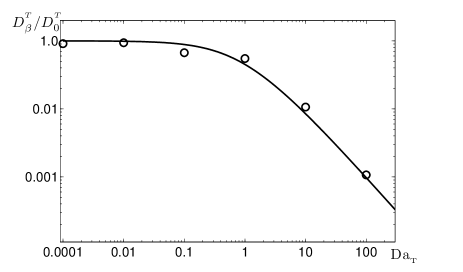
Figure 1: Comparison of the theoretical dependence of turbulent diffusion coefficient $D^{T}_{\beta}/D_{0}^{T}$ versus turbulent Damköhler number ${\rm Da}_{{}_{\rm T}}$ with the corresponding results of MFS performed in BH11 .

V Comparison with numerical simulations

In this section we compare the obtained theoretical dependence of turbulent diffusion coefficient $D^{T}_{\beta}/D_{0}^{T}$ versus turbulent Damköhler number ${\rm Da}_{{}_{\rm T}}$ with the corresponding results of MFS performed in BH11 , where a reactive front propagation in a turbulent flow was studied using the Kolmogorov-Petrovskii-Piskunov-Fisher equation. To describe the interaction with a turbulent velocity field an advection term was added to this equation, so that advection-reaction-diffusion equation reads BH11 :

$$\frac{\partial n}{\partial t}+{\bm{\nabla}\cdot}(n\,{\bm{v}})={n\over\tau_{c}}\left(1-{n\over n_{0}}\right)+D\Delta n,$$ (52)

where $n=n_{0}$ is a stable equilibrium solution of Eq. (52). After averaging Eq. (52) the following mean-field equation was obtained in BH11 :

$$\frac{\partial\overline{N}}{\partial t}+\tau\frac{\partial^{2}\overline{N}}{\partial t^{2}}={\overline{N}\over\tau_{c}}\left(1-{\overline{N}\over n_{0}}\right)+D_{\rm T}\Delta\overline{N},$$ (53)

where $D_{\rm T}$ is the sum of turbulent and molecular diffusion coefficients. The second term in the left hand side of Eq. (53) that is proportional to the memory time $\tau$, determines the memory effects of turbulent diffusion. One-dimensional Eq. (53) was solved numerically in BH11 to determine the dependence of the front speed, $s_{{}_{\rm T}}$ on turbulent Damköhler numbers. Here the reaction speed, $s_{{}_{\rm T}}=(d/dt)\int(\overline{N}/n_{0})\,dz$, is determined by differentiating the concentration integrated over the whole domain, and approximating the asymptotic front speed with the value at the time when the front has reached the other end of the computational domain.

Comparison of the theoretical dependence of turbulent diffusion coefficient versus turbulent Damköhler number with the corresponding results of MFS is shown in Fig. 1, and it demonstrate a very good agreement between the theoretical predictions [see Eqs. (43) and (44) with $\nu_{\beta}=1$ and $\alpha_{n}=1/\overline{N}_{\beta}\gg\alpha_{{}_{T}}$] and numerical simulations of BH11 . To obtain the function $D^{T}_{\beta}({\rm Da}_{{}_{\rm T}})$ we have taken into account that $s_{{}_{\rm T}}=2(D^{T}_{\beta}/\tau_{c})^{1/2}$ (see EKR98 ; BH11 ). Note that a detailed comparison of the theoretical results with DNS requires a specially designed DNS that is a subject of separate ongoing study.

VI Discussion and Conclusions

In this study we investigated effects of the chemical reactions on turbulent transport and turbulent diffusion of gaseous admixtures. To elucidate physics of the obtained results we consider examples of chemical reactions proceeding in a stoichiometric mixture. For a small concentration of reactive admixtures, $\overline{N}_{\beta}\ll\overline{N}_{f}$, the characteristic chemical time $\tau_{c}$ varies from $10^{-3}$ s to $10^{-2}$ s, where $\overline{N}_{f}$ is the ambient fluid number density. For typical values of turbulent velocity in atmospheric flows $u_{0}=1$ m/s and integral scale $\ell=100$ m, we obtain characteristic turbulent time $\tau_{0}=\ell/u_{0}=10^{2}$ s, so that the case of large turbulent Damköhler numbers, ${\rm Da}_{{}_{\rm T}}=\tau_{0}/\tau_{c}\gg 1$ is of the main physical interest. Let us also estimate the ratio $\alpha_{n}/\alpha_{{}_{T}}$ in the expression (43) for the coefficients of turbulent diffusion. Using Eq. (15), we rewrite equation for $\alpha_{{}_{T}}$ in the following form:

$$\alpha_{{}_{T}}\approx{T_{f}\over\overline{N}_{f}}\,\left({E_{a}\over R\overline{T}^{2}}\right).$$ (54)

We take into account that the temperature of the reaction products equals the fluid temperature, $\overline{T}=T_{f}$, the reactive species are strongly diluted, $\overline{N}_{\beta}\ll\overline{N}_{f}$, and $E_{a}/R\overline{T}$ varies in the range from 10 to 100. For a small enough concentration of the reactive admixtures, $\alpha_{n}/\alpha_{{}_{T}}\sim(E_{a}/R\overline{T})^{-1}(\overline{N}_{f}/\overline{N}_{\beta})\gg 1$.

The stoichiometric coefficient $\nu_{\beta}$ in Eq. (1) is known as the order of the reaction with respect to species $\beta$. In practice the overall order of the reaction is defined as the sum of the exponents of the concentrations in the reaction rate, $\nu_{c}=\sum_{\beta=1}^{m}\nu_{\beta}$. For a simplified model of a single-step reaction the overall order of the reaction is the molecularity of the reaction, indicating the number of particles entering the reaction. In general the overall order of most chemical reactions is 2 or 3, though for complex reactions the overall order of the reaction can be fractional one SP06 ; ML08 .

Let us consider first the simplest chemical reaction $A\to B$, assuming a large turbulent Damköhler numbers, ${\rm Da}_{{}_{\rm T}}\gg 1$. An example of such chemical reaction is the dissociation: $O_{2}\to O+O$. As follows from Eqs. (43) and (51), turbulent diffusion of the number density of admixtures is $D^{T}_{\beta}=D_{0}^{T}/{\rm Da}_{{}_{\rm T}}=\tau_{c}u_{0}^{2}/3$, which means that the turbulent diffusion of admixture is determined by the chemical time. This is in agreement with the result obtained in EKR98 where path-integral approach in a turbulence model with a very short correlation time was used. The underlying physics of this phenomena is quite transparent. For a simple first-order chemical reaction $A\to B$ the species $A$ of the reactive admixture are consumed and their concentration decreases much faster during the chemical reaction, so that the usual turbulent diffusion based on the turbulent time $\tau_{0}\gg\tau_{c}$, does not contribute to the mass flux of a reagent $A$. The turbulent diffusion during the turnover time of the turbulent eddies is effective only for the product of reaction, $B$. Applicability of the obtained results requires the condition ${\rm Pe}/{\rm Da}_{{}_{\rm T}}\gg 1$ to be satisfied, where ${\rm Pe}=u_{0}^{2}\tau_{0}/3$ is the Peclet number.

For multi-component second-order or third-order chemical reactions, the impact of chemistry on the turbulent diffusion is more complicated. Let us determine the turbulent diffusion coefficients for the second-order chemical reaction that is determined by the following equation:

$$A+B\to C+D.$$ (55)

An example of such chemical reaction is $H+O_{2}\to OH+O$. The numbers of species in Eq. (55) are stoichiometric coefficients, which define number of moles participating in the reaction. The stoichiometric reaction whereby the initial substances are taken in a proportion such that the chemical transformation fully converts them into the reaction products, can proceed as the inverse reaction also. For the reaction given by Eq. (55), we obtain $\alpha_{n}=2/\overline{N}$, where $\overline{N}_{A}=\overline{N}_{B}\equiv\overline{N}$. On the other hand, using Eq. (43) for the turbulent diffusion coefficients of species $A$ and $B$, we obtain

$$D_{A,B}^{T}=\frac{1}{2}\,D_{0}^{T}\,\left(1+{\rm Da}_{{}_{\rm T}}^{-1}\right).$$ (56)

Correspondingly for the third-order reaction, $A+B+C\to D+E$, we find

$$D_{A,B,C}^{T}=\frac{2}{3}\,D_{0}^{T}\,\left(1+{\rm Da}_{{}_{\rm T}}^{-1}\right),$$ (57)

where we have taken into account that in this case $\alpha_{n}=3/\overline{N}$.

Consider the stoichiometric third-order reaction with different stoichiometric coefficients of the reagents $2A+B\to 2C$ (for example, the chemical reaction $2C+O_{2}\to 2CO$ or $2H_{2}+O_{2}\to 2H_{2}O$). In this case $\alpha_{n}=2/\overline{N}$, and the turbulent diffusion coefficients of species $A$ and $B$ are as follows:

$$D_{A}^{T}=D_{0}^{T}/{\rm Da}_{{}_{\rm T}},\quad D_{B}^{T}=\frac{1}{2}\,D_{0}^{T}\,\left(1+{\rm Da}_{{}_{\rm T}}^{-1}\right).$$ (58)

Since the species $A$ have a larger stoichiometric coefficient and, correspondingly, larger number of moles participating in the chemical reaction, they are consumed more effectively in the reaction and the turbulent diffusion coefficient for the species $A$ decreases much stronger than that for species $B$.

Note that the derived in the present study theoretical dependence of turbulent diffusion coefficient versus the turbulent Damköhler number is in a good agreement with that obtained in BH11 using MFS of a reactive front propagating in a turbulent flow and described by the Kolmogorov-Petrovskii-Piskunov-Fisher equation.

The turbulent thermal diffusion coefficient in the case of a large turbulent Damköhler numbers, ${\rm Da}_{{}_{\rm T}}\gg 1$, is

$$D^{\rm TTD}_{\beta}=D_{0}^{T}\,\left[1-\nu_{\beta}\,{\overline{N}_{\beta}\over\overline{N}_{f}}\,\left({E_{a}\over R\overline{T}}\right)\,\left[1-O({\rm Da}_{{}_{\rm T}}^{-1})\right]\right],$$

(59)

which implies that the turbulent thermal diffusion is only slightly sensitive to the chemical reaction energy release in the case of small concentration of the reactive admixture, $(\overline{N}_{\beta}/\overline{N}_{f})({E_{a}}/R\overline{T})\ll 1$.

The mutual turbulent diffusion of the number density of admixtures (determined by $D_{\beta}^{\rm MTD})$ and the turbulent Duffor effect (determined by $D_{\beta}^{\rm TDE})$ are caused only by the chemical reaction, see Eqs. (45) and (49). The mechanisms of these cross-effects (e.g., heat flux caused by concentration gradient, Dufour-effect; or mutual diffusion of the number density of gaseous admixtures; or turbulent thermal diffusion) are different from molecular cross effects.

The effect of strong suppression of turbulent diffusion also holds for the heterogeneous phase transitions. It is plausible that this effect explains the existence a sharp boundary of the clouds containing very small droplets (of the order of several microns), and a visible diffusive boundary for raindrop clouds consisting of 300 - 500 microns droplets.

It should be noticed that in the case of non-stoichiometric reaction, when the substances with higher stoichiometry (molecularity) [$A$ in Eq. (58)] is excessive in the initial mixture, e.g., appears in an amount larger than that required according to the stoichiometric equation, the turbulent diffusion coefficient of the species $A$ tends to zero, so molecular diffusion can be important.

- (1) Y. B. Zeldovich, G. I. Barenblatt, V. B. Librovich, G. M. Makhviladze, The Mathematical Theory of Combustion and Explosion (Plenum, New York, 1985).
- (2) R. O. Fox, Computational Models for Turbulent Reacting Flows (Cambridge University Press, NY, 2003).
- (3) N. Peters, Turbulent Combustion (Cambridge Univ. Press, New York, 2004).
- (4) T. Echekki and E. Mastorakos, Turbulent Combustion Modeling (Springer, Dordrecht, 2011).
- (5) N. Swaminathan and K. N. C. Bray, Turbulent Premixed Flames (Cambridge Univ. Press, New York, 2011).
- (6) J. H. Seinfeld and S. N. Pandis, Atmospheric Chemistry and Physics. From Air Pollution to Climate Change, 2nd ed. (John Wiley & Sons, NY, 2006).
- (7) H. R. Pruppacher and J. D. Klett, Microphysics of Clouds and Precipitation, 2nd ed., (Kluwer Academic, Dordrecht, 1997).
- (8) P. Warneck, Chemistry of the Natural Atmosphere, (Academic Press, London, 1999).
- (9) M. Z. Jacobson, Fundamentals of Atmospheric Modeling, (Cambridge Univ. Press, Cambridge, 2005).
- (10) A. S. Monin and A. M. Yaglom, Statistical Fluid Mechanics (MIT Press, Cambridge, Massachusetts, 1975), Vol. 2.
- (11) G. T. Csanady, Turbulent Diffusion in the Environment (Reidel, Dordrecht, 1980).
- (12) W. D. McComb, The Physics of Fluid Turbulence (Clarendon, Oxford, 1990).
- (13) Ya. B. Zeldovich, A. A. Ruzmaikin, and D. D. Sokoloff, The Almighty Chance (Word Scientific Publ., Singapore, 1990).
- (14) A. K. Blackadar, Turbulence and Diffusion in the Atmosphere (Springer, Berlin, 1997).
- (15) C. T. Crowe, J. D. Schwarzkopf, M. Sommerfeld and Y. Tsuji, Multiphase flows with droplets and particles, second edition (CRC Press LLC, NY, 2011).
- (16) Z. Warhaft, Annu. Rev. Fluid Mech. 32, 203 (2000).
- (17) R. A. Shaw, Annu. Rev. Fluid Mech. 35, 183 (2003).
- (18) R. E. Britter and S. R. Hanna, Annu. Rev. Fluid Mech. 35, 469 (2003).
- (19) A. Khain, M. Pinsky, T. Elperin, N. Kleeorin, I. Rogachevskii and A. Kostinski, Atmosph. Res. 86, 1 (2007).
- (20) Z. Warhaft, Fluid Dyn. Res. 41, 011201 (2009).
- (21) S. Balachandar and J. K. Eaton, Annu. Rev. Fluid Mech. 42, 111 (2010).
- (22) T. Elperin, N. Kleeorin, I. Rogachevskii, Phys. Rev. Lett. 77, 5373 (1996).
- (23) E. Balkovsky, G. Falkovich and A. Fouxon, Phys. Rev. Lett. 86, 2790 (2001).
- (24) T. Elperin, N. Kleeorin, V. S. L’vov, I. Rogachevskii, D. Sokoloff, Phys. Rev. E 66, 036302 (2002).
- (25) G. Falkovich and A. Pumir, Phys. Fluids 16, L47 (2004).
- (26) T. Elperin, N. Kleeorin, M.A. Liberman, V.S. L’vov, I. Rogachevskii, Environ. Fluid Mech. 7, 173 (2007).
- (27) J. Salazar, J. de Jong, L. Cao, S. Woodward, H. Meng and L. Collins, J. Fluid Mech. 600, 245 (2008).
- (28) H. Xu and E. Bodenschatz, Physica D 237, 2095 (2008).
- (29) E. W. Saw, R. A. Shaw, S. Ayyalasomayajula, P. Y. Chuang and A. Gylfason, Phys. Rev. Lett. 100 214501 (2008).
- (30) A. Eidelman, T. Elperin, N. Kleeorin, B. Melnik and I. Rogachevskii, Phys. Rev. E 81, 056313 (2010).
- (31) T. Elperin, N. Kleeorin, M. A. Liberman and I. Rogachevskii, Phys. Fluids 25, 085104 (2013).
- (32) R. H. Kraichnan, Phys. Fluids 11, 945 (1968); Phys. Rev. Lett. 72, 1016 (1994).
- (33) U. Frisch, Turbulence: the Legacy of A. N. Kolmogorov (Cambridge University Press, Cambridge, 1995).
- (34) A. Donev, T. G. Fai and E. Vanden-Eijnden, J. Stat. Mech. P04004 (2014).
- (35) T. Elperin, N. Kleeorin and I. Rogachevskii, Phys. Rev. Lett. 76, 224 (1996); Phys. Rev. E 55, 2713 (1997).
- (36) T. Elperin, N. Kleeorin, I. Rogachevskii and D. Sokoloff, Phys. Rev. E 61, 2617 (2000); 64, 026304 (2001).
- (37) R. V. R. Pandya and F. Mashayek, Phys. Rev. Lett. 88, 044501 (2002).
- (38) J. Buchholz, A. Eidelman, T. Elperin, G. Grünefeld, N. Kleeorin, A. Krein, I. Rogachevskii, Experim. Fluids 36, 879 (2004).
- (39) M. W. Reeks, Int. J. Multiph. Flow 31, 93 (2005).
- (40) A. Eidelman, T. Elperin, N. Kleeorin, I. Rogachevskii and I. Sapir-Katiraie, Experim. Fluids 40, 744 (2006).
- (41) M. Sofiev, V. Sofieva, T. Elperin, N. Kleeorin, I. Rogachevskii and S. S. Zilitinkevich, J. Geophys. Res. 114, D18209 (2009).
- (42) N. E. L. Haugen, N. Kleeorin, I. Rogachevskii and A. Brandenburg, Phys. Fluids 24, 075106 (2012).
- (43) J. F. Driscoll, Progress in Energy and Combustion Science 34, 91 (2008).
- (44) D. Veynante and L. Vervisch, Progress in Energy and Combustion Science 28, 193 (2002).
- (45) R. Hilbert, F. Tap, H. El-Rabii, D. Thévenin, Progress in Energy and Combustion Science 30, 61 (2004).
- (46) M. A. Liberman, 10th International Conference on Heat Transfer, Fluid Mechanics and Thermodynamics (HEFAT-2014), keynote lecture, Orlando, Florida (2014).
- (47) T. Elperin, N. Kleeorin and I. Rogachevskii, Phys. Rev. Lett. 80, 69 (1998).
- (48) A. P. Kazantsev, Sov. Phys. JETP 26, 1031 (1968).
- (49) A. Brandenburg, N. E. L. Haugen and N. Babkovskaia, Phys. Rev. E 83, 016304 (2011).
- (50) A. N.Kolmogorov, I. G. Petrovskii, and N. S. Piskunov, Moscow Univ. Bull. Math. 1, 1 (1937).
- (51) R. A. Fisher, Ann. Eugenics 7, 353 (1937).
- (52) R. Benzi and D. R. Nelson, Physica D 238, 2003 (2009).
- (53) P. Perlekar, R. Benzi, D. R. Nelson and F. Toschi, Phys. Rev. Lett. 105, 144501 (2010).
- (54) S. A. Orszag, J. Fluid Mech. 41, 363 (1970).
- (55) A. Pouquet, U. Frisch, and J. Leorat, J. Fluid Mech. 77, 321 (1976).
- (56) S. R. de Groot and P. Mazur, Non-Equilibrium Thermodynamics (Dover, New York, 1984).
- (57) L. D. Landau and E. M. Lifshitz, Fluid Mechanics (Pergamon, Oxford, 1987).
- (58) M. Liberman, Introduction to Physics and Chemistry of Combustion (Springer-Verlag, New York, 2008).
- (59) I. Rogachevskii and N. Kleeorin, Phys. Rev. E 76, 056307 (2007).
- (60) A. Brandenburg and K. Subramanian, Phys. Rept. 417, 1 (2005).
- (61) I. Rogachevskii,N. Kleeorin, P. J. Käpylä, A. Brandenburg, Phys. Rev. E 84, 056314 (2011).
- (62) G. K. Batchelor, The Theory of Homogeneous Turbulence (Cambridge Univ. Press, New York, 1953).