Analysis of a mutualism model with stochastic perturbations

Abstract. This article is concerned with a mutualism ecological model with stochastic perturbations. The local existence and uniqueness of a positive solution are obtained with positive initial value, and the asymptotic behavior to the problem is studied. Moreover, we show that the solution is stochastically bounded, uniformly continuous and stochastic permanence. The sufficient conditions for the system to be extinct are given and the condition for the system to be persistent are also established. At last, some figures are presented to illustrate our main results.

2010 MSC: primary: 34K50, 60H10; secondary: 92B05
Keywords: It$\hat{o}$’s formula; mutualism model; Persistent in mean; Extinction; Uniformly continuous

1 Introduction

Mutualism is an important biological interaction in nature. It occurs when one species provides some benefit in exchange for some benefit, for example, pollinators and flowering plants, the pollinators obtain floral nectar (and in some cases pollen) as a food resource while the plant obtains non-trophic reproductive benefits through pollen dispersal and seed production. Another instance is ants and aphids, in which the ants obtain honeydew food resources excreted by aphids while the aphids obtain increased survival by the non-trophic service of ant defense against natural enemies of the aphids. Lots of author have discussed these models [1, 2, 3, 5, 8, 10, 12, 13, 22, 34]. One of the simplest models is the classical Lotka-Volterra two-species mutualism model as follow:

$$\left\{\begin{array}[]{lll}\dot{x}(t)=x(t)\big{(}a_{1}-b_{1}x(t)+c_{1}y(t)\big{)},\\ \dot{y}(t)=y(t)\big{(}a_{2}-b_{2}y(t)+c_{2}x(t)\big{)}.\end{array}\right.$$ (1.3)

Among various types mutualistic model, we should specially mention the following model which was proposed by May ([29]) in 1976:

$$\left\{\begin{array}[]{ll}\dot{x}(t)=x(t)\big{(}r_{1}-\frac{b_{1}x(t)}{K_{1}+y(t)}-\varepsilon_{1}x(t)\big{)},&\\ \dot{y}(t)=y(t)\big{(}r_{2}-\frac{b_{2}y(t)}{K_{2}+x(t)}-\varepsilon_{2}y(t)\big{)},&\end{array}\right.$$ (1.6)

where $x(t),y(t)$ denote population densities of each species at time t, $r_{i},K_{i},\alpha_{i},\varepsilon_{i}$ (i=1, 2) are positive constants, $r_{1},r_{2}$ denote the intrinsic growth rate of species $x(t),y(t)$ respectively, $K_{1}$ is the capability of species $x(t)$ being short of $y(t)$, similarly $K_{2}$ is the capability of species $y(t)$ being short of $x(t)$. For (1.6), there are three trivial equilibrium points

$$E_{1}=(0,0),\ \ E_{2}=(\frac{r_{1}}{\varepsilon_{1}+\frac{b_{1}}{K_{1}}},0),\ \ E_{3}=(0,\frac{r_{2}}{\varepsilon_{2}+\frac{b_{2}}{K_{2}}}),$$

and a unique positive interior equilibrium point $E^{*}=(x^{*},y^{*})$ satisfies the following equations

$$\left\{\begin{array}[]{ll}r_{1}-\frac{b_{1}x(t)}{K_{1}+y(t)}-\varepsilon_{1}x(t)=0,&\\ r_{2}-\frac{b_{2}y(t)}{K_{2}+x(t)}-\varepsilon_{2}y(t)=0,&\end{array}\right.$$ (1.9)

where $E^{*}$ is globally asymptotically stable.

In addition, population dynamics is inevitably affected by environmental noises, May[30] pointed out the fact that due to environmental fluctuation, the birth rates, carrying capacity, and other parameters involved in the model system exhibit random fluctuation to a greater or lesser extent. Consequently the equilibrium population distribution fluctuates randomly around some average values. Therefore lots of authors introduced stochastic perturbation into deterministic models to reveal the effect of environmental variability on the population dynamics in mathematical ecology [6, 9, 15, 16, 17, 20, 21, 23, 24, 25, 31, 33]. So far as our knowledge is concerned, taking into account the effect of randomly fluctuating environment, we now add white noise to each equations of the problem (1.6). Suppose that parameter $r_{i}$ is stochastically perturbed, with

$$r_{i}\rightarrow r_{i}+\alpha_{i}\dot{W}_{i}(t),\ i=1,2$$

where $W_{1}(t),W_{2}(t)$ are mutually independent Brownian motion, $\alpha_{i}^{2}$ represent the intensities of the white noise. then the corresponding deterministic model system (1.6) may be described by the It$\hat{o}$ problems:

$$\left\{\begin{array}[]{ll}dx(t)=x(t)\big{(}r_{1}-\frac{b_{1}x(t)}{K_{1}+y(t)}-\varepsilon_{1}x(t)\big{)}dt+\alpha_{1}x(t)dW_{1}(t),\\ dy(t)=y(t)\big{(}r_{2}-\frac{b_{2}y(t)}{K_{2}+x(t)}-\varepsilon_{2}y(t)\big{)}dt+\alpha_{2}y(t)dW_{2}(t).\\ \end{array}\right.$$ (1.12)

In this paper, we will discuss the stability in time average. We now briefly give an outline of the paper. In the next section, the global existence and uniqueness of the positive solution to problem (1.12) are proved by using comparison theorem for stochastic equations. Sections 3 and 4 is devoted to stochastic boundedness, uniformly Hölder-continuous. Section 5 deals with stochastic permanence. Section 6 discusses the persistence in mean and extinction, sufficient conditions of persistence in mean and extinction are obtained. Finally in section 7, we carry out numerical simulations to confirm our part results. throughout this paper, we let $(\Omega,F,{\mathcal{\{}F_{t}\}}_{t\geq 0},P)$ be a complete probability space with a filtration ${\mathcal{\{}F_{t}\}}_{t\geq 0}$ satisfying the usual conditions. $X(t)=(x(t),y(t))$ and $|X(t)|=\sqrt{x^{2}(t)+y^{2}(t)}.$

We end this section by recalling three definitions and two lemmas which we will use in the forthcoming sections.

Definition 1.1

[26] If for any $0<\varepsilon<1$, there is a constant $\delta>0$ such that the solution $(x(t),y(t))$ of (1.12) satisfies

$$\limsup_{t\rightarrow\infty}P{|X(t)|}>\delta\}<\varepsilon,$$

for any initial value $(x_{0},y_{0})>(0,0)$, then we say the solution $X(t)$ be stochastically ultimate boundedness.

Definition 1.2

[26] If for arbitrary $\varepsilon\in(0,1),$ there are two positive constants $\beta_{1}$ and $\beta_{2}$ such that for positive initial data $X_{0}=(x_{0},y_{0})$, the solution $X(t)$of problem (1.12) has the property that

$$\liminf_{t\rightarrow\infty}P\{|X(t)|\geq\beta_{1}\}\geq 1-\varepsilon,\ \ \liminf_{t\rightarrow\infty}P\{|X(t)|\leq\beta_{2}\}\geq 1-\varepsilon.\ \$$

Then problem (1.12) is said to be stochastically permanent.

Definition 1.3

[4] If $x(t),y(t)$ satisfy the following condition

$$\lim_{t\rightarrow\infty}\frac{1}{t}\int_{0}^{t}x(s)ds>0,\ \ \lim_{t\rightarrow\infty}\frac{1}{t}\int_{0}^{t}x(s)ds>0\ \ a.s.$$

The problem of (1.12) is said to be persistence in mean.

Lemma 1.1

(Chebyshev’s inequality) [28] If $\delta>0,k>0$ and $X\in L^{p}(\Omega)$ with $E|X|^{k}<\infty,$ then,

$$P\{|X|\geq\delta\}\leq\delta^{-k}E|X|^{k}.$$

Lemma 1.2

[18] Assume that an n-dimensional stochastic process $X(t)$ on $t\geq 0$ satisfies the condition

$$E|X(t)-X(s)|^{\alpha}\leq C|t-s|^{1+\beta},\ 0\leq s,\,t<+\infty$$

for some positive constants $\alpha,\beta$ and $C$. There exists a continuous modification $\tilde{X}(t)$ of $X(t)$, which has the property that for every $\gamma\in(0,\beta/\alpha)$, there is a positive random variable $h(w)$ such that

$$P\big{\{}\omega:\sup_{0<|t-s|<h(w),0\leq s,t<+\infty}\frac{|\tilde{X}(t,\omega)-\tilde{X}(s,\omega)|}{|t-s|^{\gamma}}\leq\frac{2}{1-2^{-\gamma}}\big{\}}=1.$$

In other words, almost every sample path of $\tilde{X}(t)$ is locally but uniformly Hölder-continuous with exponent $\gamma$.

2 Existence and uniqueness of the positive solution

First, we show that there exists a unique local positive solution of (1.12).

Lemma 2.1

For the given positive initial value $(x_{0},y_{0})$, there is $\tau\geq 0$ such that problem (1.12) admits a unique positive local solution $(x(t),y(t))$ a.s. for $t\in[0,\tau).$

Proof:  We first set a change of variables : $u(t)=\ln x(t),v(t)=\ln y(t)$, then problem (1.12) deduces to

$$\left\{\begin{array}[]{lll}du(t)=\big{(}r_{1}-\alpha_{1}^{2}/2-\frac{b_{1}e^{u(t)}}{K_{1}+e^{v(t)}}-\varepsilon_{1}e^{u(t)}\big{)}dt+\alpha_{1}dW_{1}(t),\\ dv(t)=\big{(}r_{2}-\alpha_{2}^{2}/2-\frac{b_{2}e^{v(t)}}{K_{2}+e^{u(t)}}-\varepsilon_{2}e^{v(t)}\big{)}dt+\alpha_{2}dW_{2}(t)\\ \end{array}\right.$$ (2.3)

on $t\geq 0$ with initial value $u(0)=\ln{x_{0}},v(0)=\ln{y_{0}}$. Obviously, the coefficients of (2.3) satisfy the local Lipschitz condition, then, making use of the theorem [7, 27] about existence and uniqueness for stochastic differential equation there is a unique local solution $(u(t),v(t))$ on $t\in[0,\tau)$, where $\tau$ is the explosion time. Hence, by It$\hat{o}$’s formula, $(x(t),y(t))$ is a unique positive local solution to problem (1.12) with positive initial value.

Next we need to prove solution is global, that is $\tau=\infty$.

Theorem 2.2

For any positive initial value $(x_{0},y_{0})$, there exists a unique global positive solution $(x(t),y(t))$ to problem (1.12), which satisfies

$$\lambda(t)\leq x(t)\leq\Lambda(t),\ \theta(t)\leq y(t)\leq\Theta(t),\ t\geq 0,\ a.s.$$

where $\lambda,\ \Lambda,\ \theta$ and $\Theta$ are defined as (2.7), (2.9), (2.13) and (2.14).

Proof:  [16]was the main source of inspiration for its proof. Because of $(x(t),y(t))$ is positive, from the first equation of (1.12) we get

$$dx(t)\leq x(t)\big{(}r_{1}-\varepsilon_{1}x(t)\big{)}dt+\alpha_{1}x(t)dW_{1}(t).$$

Define the following problem

$$\left\{\begin{array}[]{l}d\Lambda(t)=\Lambda(t)\big{(}r_{1}-\varepsilon_{1}\Lambda(t)\big{)}dt+\alpha_{1}\Lambda(t)dW_{1}(t),\\ \Lambda(0)=x_{0},\end{array}\right.$$ (2.6)

then

$$\Lambda(t)=\frac{\exp\big{(}(r_{1}-\frac{\alpha_{1}^{2}}{2})t+\alpha_{1}W_{1}(t)\big{)}}{\frac{1}{x_{0}}+\varepsilon_{1}\int^{t}_{0}\exp\big{(}(r_{1}-\frac{\alpha_{1}^{2}}{2})s+\alpha_{1}W_{1}(s)\big{)}ds}$$ (2.7)

is the unique solution of (2.6), and it follows from the comparison theorem for stochastic equations that

$$x(t)\leq\Lambda(t),\ t\in[0,\tau),\ a.s.$$

On the other hand,

$$\begin{array}[]{lll}dx(t)&\geq&x(t)\big{(}r_{1}-\frac{b_{1}x(t)}{K_{1}}-\varepsilon_{1}x(t)\big{)}dt+\alpha_{1}dW_{1}(t)\\ &=&x(t)\big{(}r_{1}-(\frac{b_{1}}{K_{1}}+\varepsilon_{1})x(t)\big{)}dt+\alpha_{1}dW_{1}(t).\end{array}$$

Obviously,

$$\lambda(t)=\frac{\exp((r_{1}-\frac{\alpha_{1}^{2}}{2})t+\alpha_{1}W_{1}(t))}{\frac{1}{x_{0}}+(\frac{b_{1}}{K_{1}}+\varepsilon_{1})\int^{t}_{0}\exp((r_{1}-\frac{\alpha_{1}^{2}}{2})s+\alpha_{1}W_{1}(s))ds}$$ (2.9)

is the solution to the problem

$$\left\{\begin{array}[]{llll}d\lambda(t)=\lambda(t)\big{(}r_{1}-(\frac{b_{1}}{K_{1}}+\varepsilon_{1})\lambda(t)\big{)}dt+\alpha_{1}\lambda(t)dW_{1}(t),\\ \lambda(0)=x_{0},\end{array}\right.$$ (2.12)

and

$$x(t)\geq\lambda(t),\ t\in[0,\tau),\ a.s.$$

Similarly, we can get

$$y(t)\leq\Theta(t),\ t\in[0,\tau),\ a.s,$$

where

$$\Theta(t)=\frac{\exp\big{(}(r_{2}-\frac{\alpha_{2}^{2}}{2})t+\alpha_{2}W_{2}(t)\big{)}}{\frac{1}{y_{0}}+\varepsilon_{2}\int^{t}_{0}\exp((r_{2}-\frac{\alpha_{2}^{2}}{2})s+\alpha_{2}W_{2}(s))ds},$$ (2.13)

and,

$$y(t)\geq\theta(t),\ t\in[0,\tau),\ a.s.$$

where

$$\theta(t)=\frac{\exp((r_{2}-\frac{\alpha_{2}^{2}}{2})t+\alpha_{2}W_{2}(t))}{\frac{1}{y_{0}}+(\frac{b_{2}}{K_{2}}+\varepsilon_{2})\int^{t}_{0}\exp((r_{2}-\frac{\alpha_{2}^{2}}{2})s+\alpha_{2}W_{2}(s))ds}.$$ (2.14)

Combining (2.13) and (2.14), we obtain

$$\lambda(t)\leq x(t)\leq\Lambda(t),\ \theta(t)\leq y(t)\leq\Theta(t),t\geq 0,\ a.s.$$

Since that $\Lambda(t),\lambda(t),\theta(t)$ and $\Theta(t)$ exist for any $t>0$, it follows from the comparison theorem for stochastic equations [14] that $(x(t),y(t))$ exists globally. $\Box$

3 Stochastically ultimate boundedness

In a population dynamical system, the nonexplosion property is often not good enough but the property of ultimate boundedness is more desired. Now, let us present a theorem about the Stochastically ultimate boundedness of (1.12) for any positive initial value.

Theorem 3.1

For any positive initial value $(x_{0},y_{0})$, the solution $X(t)$ of problem (1.12) is stochastically ultimate boundedness.

Proof:  As in [26] we define the function $U=e^{t}x^{k},\ k>0$. By the It$\hat{o}$’s formula:

$$\begin{array}[]{lll}d(e^{t}x^{k})&=&e^{t}x^{k}dt+ke^{t}x^{k-1}dx+\frac{1}{2}k(k-1)e^{t}x^{k-2}(dx)^{2}\\ &=&e^{t}x^{k}dt+ke^{t}x^{k-1}x(r_{1}-\frac{b_{1}x}{K_{1}+y}-\varepsilon_{1}x)dt+\alpha_{1}ke^{t}x^{k}dW_{1}(t)\\ &&+\frac{1}{2}k(k-1)e^{t}x^{k-1}\alpha_{1}^{2}x^{2}dt\\ &=&e^{t}x^{k}[1+k(r_{1}-\frac{b_{1}x}{K_{1}+y}-\varepsilon_{1}x)+\frac{1}{2}\alpha_{1}^{2}k(k-1)]dt+\alpha_{1}ke^{t}x^{k}dW_{1}(t).\end{array}$$

Application of young’s inequality yields,

$$\begin{array}[]{ll}&e^{t}x^{k}[1+k(r_{1}-\frac{b_{1}x}{K_{1}+y}-\varepsilon_{1}x)+\frac{1}{2}\alpha_{1}^{2}k(k-1)]\\ &\leq e^{t}[(1+kr_{1}+\frac{1}{2}\alpha_{1}^{2}k(k-1))x^{k}-k\varepsilon_{1}x^{k+1}]\\ &\leq\frac{e^{t}}{\varepsilon_{1}^{k}}\big{[}\frac{1+kr_{1}+\frac{k(k-1)}{2}\alpha_{1}^{2}}{k+1}\big{]}^{k+1}:=H_{1}(k)e^{t},\end{array}$$

where $H_{1}(k)=\frac{1}{\varepsilon_{1}^{k}}\big{[}\frac{1+kr_{1}+\frac{k(k-1)}{2}\alpha_{1}^{2}}{k+1}\big{]}^{k+1}$. Therefore,

$$d(e^{t}x^{k})\leq H_{1}(k)e^{t}dt+\alpha_{1}ke^{t}x^{k}dW_{1}(t),$$

Taking expectation to obtain

$$E(e^{t}x^{k})-E(x_{0}^{k})\leq H_{1}(k)e^{t}.$$

Thus,

$$\limsup_{t\rightarrow\infty}Ex^{k}\leq H_{1}(k).$$ (3.3)

Similarly, we have

$$\limsup_{t\rightarrow\infty}Ey^{k}\leq H_{2}(k),$$ (3.4)

where $H_{2}(k)=\frac{1}{\varepsilon_{2}^{k}}\big{[}\frac{1+kr_{2}+\frac{k(k-1)}{2}\alpha_{2}^{2}}{k+1}\big{]}^{k+1}.$ We now combine (3.3), (3.4) and the formula $\big{[}x(t)^{2}+y(t)^{2}\big{]}^{\frac{k}{2}}\leq 2^{\frac{k}{2}}\big{[}x(t)^{k}+y(t)^{k}\big{]}$ to yield

$$\limsup_{t\rightarrow\infty}E|X|^{k}\leq 2^{\frac{k}{2}}(H_{1}(k)+H_{2}(k))<+\infty.$$

By the Lemma 1.1 we can complete the proof. $\Box$

4 Uniformly Hölder-continuous

Now, let us discuss the uniformly Hölder-continuous about the positive solution of problem (1.12).

Theorem 4.1

Let $X(t)$ be a positive solution of problem (1.12) for any positive initial value $X(0)=(x_{0},y_{0})$, almost every sample path of $X(t)$ to (1.12) is uniformly Hölder-continuous.

Proof:  The proof is motivated by the arguments in [24]. The first equation of (1.12) is equivalent to the following stochastic integral equation

$$x(t)=x_{0}+\int_{0}^{t}x(s)[r_{1}-\frac{b_{1}x(s)}{K_{1}+y(s)}-\varepsilon_{1}x(s)]ds+\int_{0}^{t}\alpha_{1}x(s)dW_{1}(s).$$

By Theorem 3.2 and the inequality (3.3), we have

$$\begin{array}[]{ll}&E\big{|}x(s)[r_{1}-\frac{b_{1}x(s)}{K_{1}+y(s)}-\varepsilon_{1}x(s)]\big{|}^{k}\\ &\leq 0.5Ex^{2k}(s)+0.5E(r_{1}-\frac{b_{1}x(s)}{K_{1}+y(s)}-\varepsilon_{1}x(s))^{2k}\\ &\leq 0.5Ex^{2k}(s)+2^{2k-2}r_{1}^{2k}+2^{2k-2}Ex^{2k}(s)\\ &\leq 0.5H_{1}{(2k)}+2^{2k-2}r_{1}^{2k}+2^{2k-2}H_{1}{(2k)}\\ &=:H_{11}(k).\end{array}$$

and

$$E|\alpha_{1}x(s)|^{k}\leq\alpha_{1}^{k}H_{1}(k).$$

Using the moment inequality ([27]) gives that

$$\begin{array}[]{lll}&E|\int_{t_{1}}^{t_{2}}\alpha_{1}x(s)dW_{1}(s)|^{k}\\ &\leq\alpha_{1}^{k}[0.5k(k-1)]^{0.5k}(t_{2}-t_{1})^{0.5(k-2)}\int_{t_{1}}^{t_{2}}Ex^{k}(s)ds\\ &\leq\alpha_{1}^{k}[0.5k(k-1)]^{0.5k}(t_{2}-t_{1})^{0.5(k)}H_{1}(k)\end{array}$$

for $0\leq t_{1}\leq t_{2}$ and $k>2.$ Therefore we obtain

$$\begin{array}[]{lll}&&E|x(t_{2})-x(t_{1})|^{k}\\ &=&E\big{|}\int_{t_{1}}^{t_{2}}x(s)[r_{1}-\frac{b_{1}x(s)}{K_{1}+y(s)}-\varepsilon_{1}x(s)]ds+\int_{t_{1}}^{t_{2}}\alpha_{1}x(s)dW_{1}(s)\big{|}^{k}\\ &\leq&2^{k-1}E\big{|}\int_{t_{1}}^{t_{2}}x(s)[r_{1}-\frac{b_{1}x(s)}{K_{1}+y(s)}-\varepsilon_{1}x(s)]ds\big{|}^{k}\\ &&+2^{k-1}E\big{|}\int_{t_{1}}^{t_{2}}\alpha_{1}x(s)dW_{1}(s)\big{|}^{k}\\ &\leq&2^{k-1}(\int_{t_{1}}^{t_{2}}ds)^{k-1}\int_{t_{1}}^{t_{2}}E|x(s)[r_{1}-\frac{b_{1}x(s)}{K_{1}+y(s)}-\varepsilon_{1}x(s)]|^{k}ds\\ &&+2^{k-1}\alpha_{1}^{k}[0.5k(k-1)(t_{2}-t_{1})]^{0.5k}H_{1}(k)\\ &\leq&2^{k-1}(t_{2}-t_{1})^{k}H_{11}(k)+2^{k-1}\alpha_{1}^{k}[0.5k(k-1)(t_{2}-t_{1})]^{0.5k}H_{1}(k)\\ &\leq&2^{k-1}(t_{2}-t_{1})^{0.5k}\big{\{}(t_{2}-t_{1})^{0.5k}+[0.5k(k-1)]^{0.5k}\big{\}}H(k),\end{array}$$

for $0<t_{1}<t_{2}<\infty,t_{2}-t_{1}\leq 1,k>2,$ where $H(k)=\max\big{\{}H_{11}(k),\alpha_{1}^{k}H_{1}(k)\big{\}}.$ Hence, it follows from Lemma 1.2 that almost every sample path of $x(t)$ is locally but uniformly Hölder continuous with exponent $\gamma\in(0,\frac{k-2}{2k}),$ and almost every sample path of $x(t)$ is uniformly continuous on $t\geq 0$. Similarly, almost every sample path of $y(t)$ is uniformly continuous on $t\geq 0$. All in all, almost every sample path of $X(t)=(x(t),y(t))$ of (1.12) be uniformly continuous on $t\geq 0$. $\Box$

5 Stochastic permanence

In the study of population models, permanence is one of the most interesting and important topics. We will discuss the property by using the method as in [25] in this section.

Theorem 5.1

Problem (1.12) is stochastically permanent.

Proof:  For a positive constant $\eta<1$, we set a function

$$U(X)=\frac{1}{\eta}(1+\frac{1}{x})^{\eta}+\frac{1}{\eta}(1+\frac{1}{y})^{\eta},$$

Straightforward compute $dU(X)$ by It$\hat{o}$ formula

$$\begin{array}[]{lll}&&dU(X)\\ &=&(1+\frac{1}{x})^{\eta-1}d(\frac{1}{x})+(1+\frac{1}{y})^{\eta-1}d(\frac{1}{y})\\ &&+0.5(\eta-1)(1+\frac{1}{x})^{\eta-2}(d(\frac{1}{x}))^{2}+0.5(\eta-1)(1+\frac{1}{y})^{\eta-2}(d(\frac{1}{y}))^{2}\\ &=&(1+\frac{1}{x})^{\eta-2}\big{\{}(1+\frac{1}{x})[-\frac{1}{x}(r_{1}-\frac{b_{1}x(t)}{K_{1}+y(t)}-\varepsilon_{1}x(t))+0.5(\eta-1)\alpha_{1}^{2}\frac{1}{x^{2}}]\big{\}}dt\\ &&+(1+\frac{1}{x})^{\eta-2}\big{\{}(1+\frac{1}{x})[-\frac{1}{x}(r_{1}-\frac{b_{1}x(t)}{K_{1}+y(t)}-\varepsilon_{1}x(t))+0.5(\eta-1)\alpha_{1}^{2}\frac{1}{x^{2}}]\big{\}}dt\\ &&-\frac{1}{x}(1+\frac{1}{x})^{\eta-1}\alpha_{1}dW_{1}(t)-\frac{1}{y}(1+\frac{1}{y})^{\eta-1}\alpha_{2}dW_{2}(t)\\ &\leq&(1+\frac{1}{x})^{\eta-2}\big{\{}-\frac{1}{x^{2}}[r_{1}-0.5(\eta-1)\alpha_{1}^{2}]+\frac{1}{x}(-r_{1}+\varepsilon_{1}+\frac{b_{1}}{K_{1}})+(\varepsilon_{1}+\frac{b_{1}}{K_{1}})\big{\}}dt\\ &&+(1+\frac{1}{y})^{\eta-2}\big{\{}-\frac{1}{y^{2}}[r_{1}-0.5(\eta-1)\alpha_{1}^{2}]+\frac{1}{y}(-r_{2}+\varepsilon_{2}+\frac{b_{2}}{K_{2}})+(\varepsilon_{2}+\frac{b_{2}}{K_{2}})\big{\}}dt\\ &&-\frac{1}{x}(1+\frac{1}{x})^{\eta-1}\alpha_{1}dW_{1}(t)-\frac{1}{y}(1+\frac{1}{y})^{\eta-1}\alpha_{2}dW_{2}(t).\end{array}$$

Let us choose $\mu$ sufficiently small to satisty

$$0<\frac{\mu}{\eta}<\min\{r_{1},r_{2}\}$$

Set $V(X)=e^{\mu t}U(X),$ applying the It$\hat{o}^{,}s$ formula, we obtain

$$\begin{array}[]{lll}&&dV(X)=\mu e^{\mu t}U(X)dt+e^{\mu t}dU(X)\\ &\leq&\mu e^{\mu t}[\frac{1}{\eta}(1+\frac{1}{x})^{\eta}+\frac{1}{\eta}(1+\frac{1}{y})^{\eta}]dt+e^{\mu t}dU(X)\\ &\leq&e^{\mu t}(1+\frac{1}{x})^{\eta-2}\{-\frac{1}{x^{2}}[r_{1}-0.5(\eta-1)\alpha_{1}^{2}-\frac{\mu}{\eta}]+\frac{1}{x}(-r_{1}+\frac{2\mu}{\eta})\\ &&+(1+\frac{1}{x})(\varepsilon_{1}+\frac{b_{1}}{K_{1}})+\frac{\mu}{\eta}\}dt\\ &&+e^{\mu t}(1+\frac{1}{y})^{\eta-2}\{-\frac{1}{y^{2}}[r_{2}-0.5(\eta-1)\alpha_{2}^{2}-\frac{\mu}{\eta}]+\frac{1}{y}(-r_{2}+\frac{2\mu}{\eta})\\ &&+(1+\frac{1}{y})(\varepsilon_{2}+\frac{b_{2}}{K_{2}})+\frac{\mu}{\eta}\}dt\\ &&-e^{\mu t}[\frac{1}{x}(1+\frac{1}{x})^{\eta-1}\alpha_{1}dW_{1}(t)+\frac{1}{y}(1+\frac{1}{y})^{\eta-1}\alpha_{2}dW_{2}(t)]\\ &\leq&e^{\mu t}[(1+\frac{1}{x})^{\eta-1}(\varepsilon_{1}+\frac{b_{1}}{K_{1}}+\frac{\mu}{\eta})+(1+\frac{1}{y})^{\eta-1}(\varepsilon_{2}+\frac{b_{2}}{K_{2}}+\frac{\mu}{\eta})]dt\\ &&-e^{\mu t}[\frac{1}{x}(1+\frac{1}{x})^{\eta-1}\alpha_{1}dW_{1}(t)+\frac{1}{y}(1+\frac{1}{y})^{\eta-1}\alpha_{2}dW_{2}(t)]\\ &\leq&L_{1}e^{\mu t}dt-e^{\mu t}[\frac{1}{x}(1+\frac{1}{x})^{\eta-1}\alpha_{1}dW_{1}(t)+\frac{1}{y}(1+\frac{1}{y})^{\eta-1}\alpha_{2}dW_{2}(t)],\end{array}$$

where $L_{1}=\max\{\varepsilon_{1}+\frac{b_{1}}{K_{1}}+\frac{\mu}{\eta},\varepsilon_{2}+\frac{b_{2}}{K_{2}}+\frac{\mu}{\eta}\}.$

Integrating and then taking expectations yields

$$E[V(X)]=e^{\mu t}E(U(X))\leq\frac{1}{\eta}(1+\frac{1}{x_{0}})^{\eta}+\frac{1}{\eta}(1+\frac{1}{y_{0}})^{\eta}+\frac{L_{1}}{\mu}(e^{\mu t}-1).$$

Therefore,

$$\limsup_{t\rightarrow+\infty}E[\frac{1}{x^{\eta}(t)}]\leq\limsup_{t\rightarrow+\infty}E[(1+\frac{1}{x(t)})^{\eta}+(1+\frac{1}{y(t)})^{\eta}]\leq\frac{\eta L_{1}}{\mu}=L,$$

and

$$\limsup_{t\rightarrow+\infty}E[\frac{1}{y^{\eta}(t)}]\leq\limsup_{t\rightarrow+\infty}E[(1+\frac{1}{x(t)})^{\eta}+(1+\frac{1}{y(t)})^{\eta}]\leq\frac{\eta L_{1}}{\mu}=L.$$

For arbitrary $\varepsilon\in(0,1)$, choose $\beta_{1}(\varepsilon)=(\frac{\varepsilon}{L})^{\frac{1}{\eta}},$ we yield the following inequality making Chebyshev’s inequality,

$$P\{x(t)<\beta_{1}\}=P\{\frac{1}{x^{\eta}(t)}>\frac{1}{\beta_{1}^{\eta}}\}\leq\frac{E[\frac{1}{x^{\eta}(t)}]}{\beta_{1}^{-\eta}},$$

$$P\{y(t)<\beta_{1}\}=P\{\frac{1}{y^{\eta}(t)}>\frac{1}{\beta_{1}^{\eta}}\}\leq\frac{E[\frac{1}{y^{\eta}(t)}]}{\beta_{1}^{-\eta}}.$$

Hence,

$$\limsup_{t\rightarrow+\infty}P\{|X(t)|<\beta_{1}\}\leq\beta_{1}^{\eta}L=\varepsilon,$$

Then,

$$\liminf_{t\rightarrow+\infty}P\{|X(t)|\geq\beta_{1}\}\geq 1-\varepsilon.$$

Using Chebyshev’s inequality and (3.3), (3.4) we can prove that
for arbitrary $\varepsilon\in(0,1)$, there is a positive constant $\beta_{2}$ such that

$$\liminf_{t\rightarrow+\infty}P\{|X(t)|\leq\beta_{2}\}\geq 1-\varepsilon.$$

$\Box$

6 Persistence in mean and extinction

In the description of population dynamics, it is critical to discuss the property of persistence in mean and extinction.

Theorem 6.1

Suppose that $r_{i}>\frac{\alpha_{i}^{2}}{2},(i=1,2),$ $X(t)$ is the positive solution to (1.12) with positive initial value $(x_{0},y_{0})$, then the problem (1.12) is persistent in mean.

Proof:  The method is similar to [16]. We first deduce

$$\lim_{t\rightarrow\infty}\frac{\ln x(t)}{t}=0,\ \lim_{t\rightarrow\infty}\frac{\ln y(t)}{t}=0.$$

For $t\geq T>0$, we compute from (2.7) that

$$\Lambda(t)=\frac{\exp\big{(}(r_{1}-\frac{\alpha_{1}^{2}}{2})(t-T)+\alpha_{1}(W_{1}(t)-W_{1}(T))\big{)}}{\frac{1}{x(T)}+\varepsilon_{1}\int^{t}_{T}\exp\big{(}(r_{1}-\frac{\alpha_{1}^{2}}{2})s+\alpha_{1}W_{1}(s)\big{)}ds}.$$

Hence,

$$\begin{array}[]{lll}&&\frac{1}{\Lambda(t)}=\frac{\frac{1}{x(T)}+\varepsilon_{1}\int^{t}_{T}\exp\big{(}(r_{1}-\frac{\alpha_{1}^{2}}{2})s+\alpha_{1}W_{1}(s)\big{)}ds}{\exp\big{(}(r_{1}-\frac{\alpha_{1}^{2}}{2})(t-T)+\alpha_{1}(W_{1}(t)-W_{1}(T))\big{)}}\\ &\geq&\exp\big{(}-(r_{1}-\frac{1}{2}\alpha_{1}^{2})(t-T)-\alpha_{1}(W_{1}(t)-W_{1}(T))\big{)}\times\\ &&\big{[}\frac{1}{x(T)}+\varepsilon_{1}\int^{t}_{T}\exp((r_{1}-\frac{\alpha_{1}^{2}}{2})v+\alpha_{1}W_{1}(v))dv\big{]}\\ &\geq&\frac{\varepsilon_{1}}{r_{1}-\frac{\alpha_{1}^{2}}{2}}\exp\big{(}(r_{1}-\frac{\alpha_{1}^{2}}{2})T+\alpha_{1}W_{1}(T)\big{)}\big{(}1-\exp(-(r_{1}-\frac{\alpha_{1}^{2}}{2})(t-T))\big{)}\times\\ &&\exp\big{(}\alpha_{1}(\min_{0\leq v\leq t}W_{1}(v)-\max_{0\leq v\leq t}W_{1}(v))\big{)}\\ &=:&H_{1}(t)\exp\big{(}\alpha_{1}(\min_{0\leq v\leq t}W_{1}(v)-\max_{0\leq v\leq t}W_{1}(v))\big{)},\end{array}$$

where $H_{1}(t)=\frac{\varepsilon_{1}}{r_{1}-\frac{\alpha_{1}^{2}}{2}}e^{(r_{1}-\frac{\alpha_{1}^{2}}{2})T+\alpha_{1}W_{1}(T)}\big{(}1-e^{-(r_{1}-\frac{\alpha_{1}^{2}}{2})(t-T)}\big{)}.$
Taking logarithm to obtain

$$-\ln\Lambda(t)\geq\ln H_{1}(t)+\alpha_{1}\big{(}\min_{0\leq v\leq t}W_{1}(v)-\max_{0\leq v\leq t}W_{1}(v)\big{)},$$

which implies that

$$\frac{\ln\Lambda(t)}{t}\leq-\frac{\ln H_{1}(t)}{t}-\alpha_{1}\frac{\min_{0\leq v\leq t}W_{1}(v)-\max_{0\leq v\leq t}W_{1}(v)}{t}.$$

The distributions of $\max_{0\leq v\leq t}W_{1}(v),$ is same as $|W_{1}(t)|$, $\min_{0\leq v\leq t}W_{1}(v)$ have same distribution as $-\max_{0\leq v\leq t}W_{1}(v).$ Moreover, $\frac{\ln H_{1}(t)}{t}\rightarrow\infty$ as $t\rightarrow\infty,$ by the strong law of large numbers we get $\lim_{t\rightarrow\infty}\sup\frac{\ln\Lambda(t)}{t}\leq 0.$ Then

$$\lim_{t\rightarrow\infty}\sup\frac{\ln x(t)}{t}\leq 0.$$

On the other hand, from the (2.9) we have:

$$\frac{1}{\lambda(t)}=\frac{1}{x_{0}}e^{-(r_{1}-\frac{\alpha_{1}^{2}}{2})t-\alpha_{1}W_{1}(t)}+(\frac{b_{1}}{K_{1}}+\varepsilon_{1})\int_{0}^{t}e^{-(r_{1}-\frac{\alpha_{1}^{2}}{2})(t-s)-\alpha_{1}(W_{1}(t)-W_{1}(s))}ds$$

$$\leq e^{\alpha_{1}(\max_{0\leq s\leq t}W_{1}(s)-W_{1}(t))}\big{[}\frac{1}{x_{0}}e^{-(r_{1}-\frac{\alpha_{1}^{2}}{2})t}+(\frac{b_{1}}{K_{1}}+\varepsilon_{1})\int_{0}^{t}e^{-(r_{1}-\frac{\alpha_{1}^{2}}{2})(t-s)}ds\big{]}.$$

Similarly, we can deduce

$$\frac{1}{\lambda(t)}\geq e^{\alpha_{1}(\min_{0\leq s\leq t}W_{1}(s)-W_{1}(t))}\big{[}\frac{1}{x_{0}}e^{-(r_{1}-\frac{\alpha_{1}^{2}}{2})t}+(\frac{b_{1}}{K_{1}}+\varepsilon_{1})\int_{0}^{t}e^{-(r_{1}-\frac{\alpha_{1}^{2}}{2})(t-s)}ds\big{]}.$$

Note that

$$\eta(t)=\frac{1}{\frac{1}{x_{0}}e^{-(r_{1}-\frac{\alpha_{1}^{2}}{2})t}+(\frac{b_{1}}{K_{1}}+\varepsilon_{1})\int_{0}^{t}e^{-(r_{1}-\frac{\alpha_{1}^{2}}{2})(t-s)}ds}$$

is the solution of the problem

$$\left\{\begin{array}[]{llll}\dot{\eta}(t)=\eta(t)\big{(}r_{1}-\frac{\alpha_{1}^{2}}{2}-(\frac{b_{1}}{K_{1}}+\varepsilon_{1})\eta(t)\big{)},\\ \eta(0)=x_{0},\end{array}\right.$$ (6.4)

we have

$$e^{\alpha_{1}(\min_{0\leq s\leq t}W_{1}(s)-W_{1}(t))}\frac{1}{\eta(t)}\leq\frac{1}{\lambda(t)}\leq e^{\alpha_{1}(\max_{0\leq s\leq t}W_{1}(s)-W_{1}(t))}\frac{1}{\eta(t)},$$

that is

$$\alpha_{1}(W_{1}(t)-\max_{0\leq s\leq t}W_{1}(s))\leq\ln\lambda(t)-\ln\eta(t)\leq\alpha_{1}(W_{1}(t)-\min_{0\leq s\leq t}W_{1}(s)).$$

Making use of the large number theorem and the distribution of $|W_{1}(t)|$, we get

$$\lim_{t\rightarrow\infty}\frac{\ln\lambda(t)}{t}=0,$$

Therefore

$$\lim_{t\rightarrow\infty}\sup\frac{\ln x(t)}{t}\geq 0.$$

Hence,

$$\lim_{t\rightarrow\infty}\frac{\ln x(t)}{t}=0.$$

Similarly, we yield that

$$\lim_{t\rightarrow\infty}\frac{\ln y(t)}{t}=0.$$

Integrating the first equation of (2.1) from $0$ to $t$, we yield

$$b_{1}\int_{0}^{t}\frac{x(s)}{K_{1}+y(s)}ds=-(\ln x(t)-\ln x_{0})+(r_{1}-\frac{\alpha_{1}^{2}}{2})t+\alpha_{1}W_{1}(t)-\varepsilon_{1}\int_{0}^{t}x(s)ds,$$

because of $\int_{0}^{t}x(s)ds\geq K_{1}\int_{0}^{t}\frac{x(s)}{K_{1}+y(s)}ds,$ we obtain

$$b_{1}\frac{1}{t}\int_{0}^{t}x(s)ds\geq K_{1}\frac{1}{t}\big{[}-(\ln x(t)-\ln x_{0})+(r_{1}-\frac{\alpha_{1}^{2}}{2})t+\alpha_{1}W_{1}(t)-\varepsilon_{1}\int_{0}^{t}x(s)ds\big{]},$$

that is

$$(b_{1}+\varepsilon_{1}K_{1})\frac{1}{t}\int_{0}^{t}x(s)ds\geq-K_{1}\frac{\ln x(t)-\ln x_{0}}{t}+K_{1}(r_{1}-\frac{\alpha_{1}^{2}}{2})+K_{1}\alpha_{1}\frac{W_{1}(t)}{t}.$$

Since that $\lim_{t\rightarrow\infty}\frac{W_{1}(t)}{t}=0$, and $\lim_{t\rightarrow\infty}\frac{\ln x(t)}{t}=0$, we get

$$\lim_{t\rightarrow\infty}\frac{\int_{0}^{t}x(s)ds}{t}\geq\frac{K_{1}(r_{1}-\frac{\alpha_{1}^{2}}{2})}{b_{1}+\varepsilon_{1}K_{1}}>0,\ a.s.$$

Similarly, we yield

$$\lim_{t\rightarrow\infty}\frac{\int_{0}^{t}y(s)ds}{t}\geq\frac{K_{2}(r_{2}-\frac{\alpha_{2}^{2}}{2})}{b_{2}+\varepsilon_{2}K_{2}}>0,\ a.s.$$

The proof is completed $\Box$

Theorem 6.2

Let $X(t)=(x(t),y(t))$ be a positive solution of (1.12) with positive initial value $X(0)=(x_{0},y_{0})$, then
$(A)$ If $r_{1}<\frac{\alpha_{1}^{2}}{2},r_{2}>\frac{\alpha_{2}^{2}}{2}$, then $x(t)$ is extinction, $y(t)$ is persistent in mean.
$(B)$ If $r_{1}>\frac{\alpha_{1}^{2}}{2},r_{2}<\frac{\alpha_{2}^{2}}{2}$, then $y(t)$ is extinction, $x(t)$ is persistent in mean.
$(C)$ If $r_{1}<\frac{\alpha_{1}^{2}}{2},r_{2}<\frac{\alpha_{2}^{2}}{2}$, then $x(t),y(t)$ be extinction.

Proof:  We first prove part $(A)$ of the theorem. The proof of $(B),(C)$ is similar. It follows from the first equation of (2.1) that

$$du(t)\leq(r_{1}-\frac{\alpha_{1}^{2}}{2})dt+\alpha_{1}dW_{1}(t).$$

Apply the comparison theorem for stochastic equations and the diffusion processes, we deduce that

$$\lim_{t\rightarrow\infty}u(t)=-\infty,$$

i.e.

$$\lim_{t\rightarrow\infty}x(t)=0,\ a.s.$$

Hence for any small $\varepsilon>0$, there exist $t_{0}$ and a set $\Omega_{\varepsilon}$ such that $P(\Omega_{\varepsilon})\geq 1-\varepsilon$ and $\frac{x(t)}{K_{2}+x(t)}\leq\varepsilon$ for $t\geq t_{0}$ and $\omega\in\Omega_{\varepsilon}.$ Therefore, the second equation of (1.12) becomes

$$dy(t)=y(t)\big{(}r_{2}-\frac{b_{2}y(t)}{K_{2}+x(t)}-\varepsilon_{2}y(t)\big{)}dt+\alpha_{2}y(t)dW_{2}(t)$$

$$=y(t)\big{(}r_{2}-\frac{b_{2}y(t)}{K_{2}}+\frac{b_{2}y(t)x(t)}{K_{2}(K_{2}+x(t))}-\varepsilon_{2}y(t)\big{)}dt+\alpha_{2}y(t)dW_{2}(t).$$

We can yield

$$y(t)\geq y(t)\big{(}r_{2}-(\frac{b_{2}}{K_{2}}+\varepsilon_{2})y(t)\big{)}dt+\alpha_{2}y(t)dW_{2}(t),$$

$$y(t)\leq y(t)\big{(}r_{2}-(\frac{b_{2}}{K_{2}}(1-\varepsilon)+\varepsilon_{2})y(t)\big{)}dt+\alpha_{2}y(t)dW_{2}(t).$$

If $r_{2}>\frac{\alpha_{2}^{2}}{2},$ using comparison theorem for stochastic equations, we get

$$\lim_{t\rightarrow\infty}\inf\frac{\int_{0}^{t}y(s)ds}{t}\geq\frac{r_{2}-\frac{\alpha_{2}^{2}}{2}}{\frac{b_{2}}{K_{2}}+\varepsilon_{2}},\ \lim_{t\rightarrow\infty}\sup\frac{\int_{0}^{t}y(s)ds}{t}\leq\frac{r_{2}-\frac{\alpha_{2}^{2}}{2}}{\frac{b_{2}(1-\varepsilon)}{K_{2}}+\varepsilon_{2}},$$

which implies that

$$\lim_{t\rightarrow\infty}\frac{\int_{0}^{t}y(s)ds}{t}=\frac{r_{2}-\frac{\alpha_{2}^{2}}{2}}{\frac{b_{2}}{K_{2}}+\varepsilon_{2}}>0,\ \ a.s.$$

That is $y(t)$ is persistent in mean.

$\Box$

7 Numerical simulations

Now let us make use of Milstein’s method [11] to illustrate the analytical findings. Consider the following discretization system:

$$\left\{\begin{array}[]{lll}x^{(n+1)}&=&x^{(n)}+x^{(n)}\big{(}r_{1}-\frac{b_{1}x^{(n)}}{K_{1}+y^{(n)}}-\varepsilon_{1}x^{(n)}\big{)}\Delta t+\alpha_{1}x^{(n)}\sqrt{\Delta t}\xi^{(n)}\\ &&+\frac{\alpha_{1}^{2}}{2}x^{(n)}((\xi^{(n)})^{2}-1)\Delta t,\\ y^{(n+1)}&=&y^{(n)}+y^{(n)}\big{(}r_{2}-\frac{b_{2}y^{(n)}}{K_{2}+x^{(n)}}-\varepsilon_{2}y^{(n)}\big{)}\Delta t+\alpha_{2}y^{(n)}\sqrt{\Delta t}\zeta^{(n)}\\ &&+\frac{\alpha_{2}^{2}}{2}y^{(n)}((\zeta^{(n)})^{2}-1)\Delta t,\end{array}\right.$$ (7.5)

where $\xi^{(n)}$ and $\zeta^{(n)},$ n=1, 2, …, N, are the Gaussian random variables $N(0,1)$. In Figure 1 we choose $r_{1}=1.2,r_{2}=1,\varepsilon_{1}=0.8,\varepsilon_{2}=0.7,b_{1}=0.7,b_{2}=0.9,K_{1}=K_{2}=2$, step size $\Delta$ t=0.001. The only difference between conditions of Figure 1 is that the value of $\alpha_{1},\alpha_{2}$ . In Figure 1 (a), we choose $\alpha_{1}=\alpha_{2}=0$, we can see the positive equilibrium point $E^{*}$ is globally stable; In Figure 1 (b)-(d)we choose the value of $\alpha_{1},\alpha_{2}$ such that $r_{1}<\frac{\alpha_{1}^{2}}{2},r_{2}<\frac{\alpha_{2}^{2}}{2};r_{1}>\frac{\alpha_{1}^{2}}{2},r_{2}<\frac{\alpha_{2}^{2}}{2};r_{1}>\frac{\alpha_{1}^{2}}{2},r_{2}>\frac{\alpha_{2}^{2}}{2}$ respectively, then in view Theorem 6.2, we confirms them. By comparing In Figure 1 (a), (b), (c), we can see that small random perturbation can retain the stochastic system permanent; sufficiently large random perturbation leads to the stochastic system extinct.

(a)(b) (c)(d)

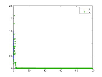
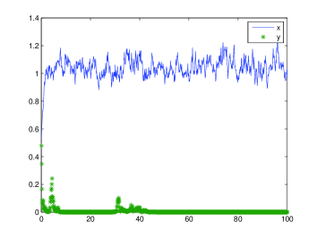
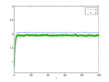
Figure 1: Solutions of (1.12) for $r_{1}=1.2,r_{2}=1,\varepsilon_{1}=0.8,\varepsilon_{2}=0.7,b_{1}=0.7,b_{2}=0.9,K_{1}=K_{2}=2$, step size $\Delta$ t=0.001. (a) is with $\alpha_{1}=\alpha_{2}=0$; (b) is with $\alpha_{1}=2.2,\alpha_{2}=1.8$; (c) is with $\alpha_{1}=0.1,\alpha_{2}=1.6$; (d) is with $\alpha_{1}=0.01,\alpha_{2}=0.01.$

References

[1]
E. S. Allman and J. A. Rhodes, ”Mathematical Models in Biology: An Introduction”, Cambridge University Press, 2004.
[2]
D. H. Boucher, S. James and K. H. Keeler, The ecology of mutualisms, it Annual Review of Ecology and Systematics 13 (1982), 315-347.
[3]
F. D. Chen, Permanence of a delayed discrete mutualism model with feedback controls, Math. Comput. Model.50 (2009), 1083-1089.
[4]
L. Chen, J. Chen, Nonlinear biological dynamical system, Science Press, Beijing, 1993.
[5]
F. D. Chen, M. S. You, Permanence for an integrodifferential model of mutualism, Appl. Math. Comput.186 (2007), 30-34.
[6]
N. H. Du, V. H. Sam, Dynamics of a stochastic Lotka-Volterra model perturbed by white noise, J. Math. Anal. Appl.324 (2006), 82-97.
[7]
A. Friedman, Stochastic differential equations and their applications, Academic press, New York, 1976.
[8]
B. S. Goh, Stability in models of mutualism, Amer. Natural.113 (1979), 261-275.
[9]
Y. Hu, F. Wu and C. Huang, Stochastic Lotka-Volterra models with multiple delays, J. Math. Anal. Appl.375 (2011), 42-57.
[10]
V. Hutson, K. Schmitt, Permanence and the dynamics of biological systems, Math. Biosci.111
(1992), 1-71.
[11]
D. J. Higham, An algorithmic introduction to numerical simulation of stochastic differential equations,
SIAM Rev.43 (2001), 525-546.
[12]
J. N. Holland, D. L. DeAngelis and J. L. Bronstein, Population dynamics and mutualism: Functional responses of benefits and costs,
The Amer. Natural.159 (2002), 231-244.
[13]
J. N. Holland, D. L. DeAngelis, A consumer-resource approach to the density-dependent population dynamics of mutualism,
Ecology.91 (2010), 1286-1295.
[14]
N. Ikeda, S. Wantanabe, Stochastic differential equations and diffusion processes, North-Holland, Amsterdam, 1981.
[15]
D. Q. Jiang, N. Z. Shi and X. Y. Li, Global stability and stochastic permanence of a non-autonomous logistic equation with
random perturbation, J. Math. Anal. Appl.340 (2008), 588-597.
[16]
C. Y. Ji, D. Q. Jiang and N. Z. Shi, Analysis of a predator-prey model with modified Leslie-Gower and Holling-
type II schemes with stochastic perturbation, J. Math. Anal. Appl.359 (2009), 482-489.
[17]
C. Y. Ji, D. Q. Jiang, Persistence and non-persistence of a mutualism system with stochastic perturbation,
Discrete Contin. Dyn. Syst.32 (2012), 867-889.
[18]
I. Karatzas, S. E. Shreve, ”Brownian Motion and Stochastic Calculus”, Springer-Verlag, Berlin, 1991.
[19]
F. C. Klebaner, Introduction to stochastic calculus with applications, Imperial college press, 1998.
[20]
X. Li, A. Gray, D, Jiang and X. Mao, Sufficient and necessary conditions of stochastic permanence
and extinction for stochastic logistic populations under regime switching, J. Math. Anal. Appl.376 (2011), 11-28.
[21]
G. Lu, Z. Lu and X. Lian, Delay effect on the permanence for Lotka-Volterra cooperative systems,
Nonl. Anal. RWA.11 (2010), 2810-2816.
[22]
Z. Lu, Y. Takeuchi, permanence and global stability for cooperative Lotka-Volterra diffusion systems,
Nonl. Anal.19 (1992), 963-975.
[23]
M. Liu, K. Wang, Survival analysis of a stochastic cooperation system in a polluted environment,J. Biol. Syst.19 (2011), 183-204.
[24]
M. Liu, K. Wang, Population dynamical behavior of Lotka-Volterra cooperative systems with random perturbations,
Disc. Cont. Dyna. Systems.33 (2013), 2495-2522.
[25]
M. Liu, K. Wang, Analysis of a stochastic autonomous mutualism model, J. Math. Anal. Appl.402 (2013), 392-403.
[26]
X. Y. Li, X. R. Mao, Population dynamical behavior of non-autonomous Lotka-Volterra competitive system
with random perturbations, Disc. Cont. Dyna. Systems.24 (2009), 523-545.
[27]
X. R. Mao, Stochastic Differential Equations and Applications, Horwood, Chichester,
1997.
[28]
X. R. Mao, C. Yuan, Stochastic Differential Equations with markovian switching, Imperial College press, 2006
[29] R. M. May, ”Models of two interacting populations”, in Theoretical Ecology: Principles and Application, ed. R. M. May (Philadelphia,
PA: Saunders, 1976) 78-104.
[30] R. M. May, Stability and complexity in model ecosystems, Princeton University Press, NJ, 2001
[31]
X. Mao, S. Sabais and E. Renshaw, Asymptotic behavior of stochastic Lotka-Volterra model, J. Math. Anal. Appl.287 (2003), 141-156.
[32]
S. Pang, F. Deng and X. Mao, Asymptotic properties of stochastic population dynamics,
Disc. Cont. Dyna. Systems15 (2008), 603-620.
[33]
Y. Takeuchi, N.H. Dub, N.T. Hieu, K. Sato, Evolution of predator-prey systems described by a Lotka-Volterra equation under random environment,
J. Math. Anal. Appl.323 (2006), 938-957.
[34]
A. R. Thompson, R. M. Nisbet and R. J. Schmitt, Dynamics of mutualist populations that are demographically open, J. Anim. Ecol. 75 (2006), 1239-1251.