Predicted Space Motions for Hypervelocity and Runaway Stars: Proper Motions and Radial Velocities for the GAIA Era

Abstract

We predict the distinctive three dimensional space motions of hypervelocity stars (HVSs) and runaway stars moving in a realistic Galactic potential. For nearby stars with distances less than 10 kpc, unbound stars are rare; proper motions alone rarely isolate bound HVSs and runaways from indigenous halo stars. At large distances of 20–100 kpc, unbound HVSs are much more common than runaways; radial velocities easily distinguish both from indigenous halo stars. Comparisons of the predictions with existing observations are encouraging. Although the models fail to match observations of solar-type HVS candidates from SEGUE, they agree well with data for B-type HVS and runaways from other surveys. Complete samples of $g\lesssim$ 20 stars with GAIA should provide clear tests of formation models for HVSs and runaways and will enable accurate probes of the shape of the Galactic potential.

1 INTRODUCTION

From the Galactic Center (GC) to the Magellanic Clouds, three dimensional (3D) space motions yield interesting information on the mass distribution and stellar populations in the Local Group. At the GC, proper motion and radial velocity data for several dozen bright O-type and B-type stars orbiting Sgr A^∗ reveal the existence of a black hole with a mass of roughly $4\times 10^{6}$ $M_{\odot}$ (e.g., Genzel et al., 2010; Morris et al., 2012). For the LMC, 3D motions of several thousand stars allow measures of the orientation of the stellar disk and the mass contained within $\sim$ 9 kpc (van der Marel & Kallivayalil, 2014). On distance scales intermediate between these two extremes, accurate space motions of large groups of stars bound to the Milky Way measure (i) the rotation of the Galactic bulge (e.g., Soto et al., 2014), (ii) the kinematics of nearby OB associations in the Galactic disk (e.g., de Zeeuw et al., 1999; Reid et al., 2014), and (iii) the frequency of streams of stars in the Milky Way halo (Koposov et al., 2013).

Unbound stars ejected from the Milky Way can also probe Galactic structure. HVSs are ejected from the GC when a close binary system passes within the tidal boundary of the central supermassive black hole (SMBH; Hills, 1988). During this passage, one component of the binary becomes bound to the SMBH; to conserve energy, the other is ejected at velocities ranging from a few hundred to a few thousand km s^-1. Robust identification of unbound HVSs in the halo enables more accurate measurements of the total mass of the Milky Way (e.g., Brown et al., 2010b; Gnedin et al., 2010). Because HVSs leave the GC on nearly radial orbits, measuring the 3D trajectories of unbound HVSs in the halo constrain the anisotropy of the Galactic potential (e.g., Gnedin et al., 2005; Yu & Madau, 2007).

Space motions of runaway stars may provide additional constraints on the Galactic potential (e.g., Martin, 2006). Produced when one component of a binary system explodes as a supernova (Zwicky, 1957; Blaauw, 1961) or when a star receives kinetic energy through dynamical interactions with several more massive stars (e.g., Poveda et al., 1967; Leonard, 1991), high velocity runaways have space motions and spatial distributions distinct from HVSs (Martin, 2006; Bromley et al., 2009). Separating unbound HVSs from unbound runaways should enable more rigorous constraints on the mass of the Galaxy and any anisotropy in the Galactic potential.

Realizing these possibilities requires robust predictions for the space motions of HVSs and runaways moving through a realistic Galactic potential. Here, we focus on calculations in an axisymmetric potential. Our results demonstrate that proper motions (radial velocities) isolate nearby (distant) HVSs and runaways from indigenous stars. Unique variations of proper motion and radial velocity with Galactic longitude and latitude enable new ways to identify high velocity stars. For observed high velocity stars, comparisons with the models indicate a mix of HVSs and runaways, with a strong preference for an HVS origin among the most distant stars.

2 OVERVIEW

To predict proper motions and radial velocities for HVSs and runaways, we consider both analytic models and numerical simulations. For stars with specific trajectories, analytic models allow us to derive the variations in proper motion and radial velocity as a function of position in the Galaxy. Numerical simulations yield predictions for the distributions of positions and space motions for specific models of HVSs and runaways.

We begin in §3 with a formal discussion of the analytic model. After defining cartesian, cylindrical, and spherical coordinate systems (§3.1), we derive radial and tangential velocities for stars (i) orbiting the Galaxy (§3.2.1) and (ii) moving radially away from the GC (§3.2.2). Features in the behavior of the radial and tangential velocities with distance and Galactic coordinates provide a basis for differentiating the two types of motion.

Readers more interested in results than techniques can use the figures in §3 as a guide and concentrate on §3.3, where we summarize the relative value of radial velocities and proper motions for identifying HVSs and runaways among indigenous stars. For stars at distances $d\gtrsim$ 20 kpc from the Sun, radial velocities separate orbital motion from radial motion. For nearby stars ($d\lesssim$ 20 kpc), tangential velocities may discriminate ejected stars from bulge and disk stars, but probably cannot isolate ejected stars from halo stars.

In §4, we describe numerical techniques for simulating HVSs and runaways moving through the Galaxy. Our procedures follow those discussed in Bromley et al. (2006), Kenyon et al. (2008), and Bromley et al. (2009). Here, we focus on the input gravitational potential for the Galaxy (§4.1), the initial conditions (§4.2), and the integration technique (§4.3).

We discuss results in four sections. We start by considering the fraction of ejected stars which reach the outer Galaxy with Galactocentric distances $r\gtrsim$ 60 kpc and high Galactic latitude, $|b|\gtrsim$ 30^o (§5). With their large ejection velocities, 25% of HVSs reach the outer halo. Much smaller ejection velocities prevent a large fraction of runaways from leaving the inner disk. For supernova-induced (dynamically ejected) runaways, only 1% (0.25%) reach Galactocentric distances of 60 kpc. Roughly 0.1% of either type of runaway achieves Galactocentric distances of 60 kpc and $|b|\gtrsim$ 30^o.

In §6, we examine distributions of the proper motion $\mu$ and radial velocity $v_{r}$ for complete samples of stars produced in simulations of HVSs and runaways. After exploring the density of stars in the $d-\mu$ (§6.1) and the $d-v_{r}$ (§6.2) planes, we examine the distributions of radial velocity and proper motion in specific distance bins and distributions of proper motion for all stars in each simulation (§6.3) and the density of stars as a function of Galactic coordinates (§6.4). §6.5 briefly summarizes the highlights of these simulations.

To establish predictions for surveys with GAIA and other facilities, we continue by constructing magnitude-limited samples of HVSs and runaways for 1 $M_{\odot}$ and 3 $M_{\odot}$ stars (§7). In the $v_{r}-\mu$ plane, magnitude-limited samples of nearby, mostly bound HVSs and runaways with d $\lesssim$ 10 kpc have nearly identical distributions, complicating attempts to isolate these stars from the indigenous halo population. Among 3 $M_{\odot}$ stars, high velocity HVSs easily distinguish themselves from high velocity runaways.

Comparisons between the numerical results and observations of several sets of high velocity stars complete our analysis (§8). HVS and runaway models yield a poor match to observations of solar-type HVS candidates from SEGUE (§8.1; Palladino et al., 2014). However, the models provide an excellent match to observations of B-type HVS candidates (§8.2; Brown et al., 2014), nearby B-type runaways (§8.3; Silva & Napiwotzki, 2011), and miscellaneous HVS and runaway star candidates from other surveys (§8.4; Edelmann et al., 2005; Heber et al., 2008; Tillich et al., 2009; Irrgang et al., 2010; Zheng et al., 2014). Although radial velocities easily separate unbound HVSs and runaways from indigenous halo stars, kinematic data alone are not sufficient to isolate bound HVSs or runaways from halo stars (§8.5). Combined with estimates of production rates (§8.6), these results suggest that ejections from the GC are the source of the highest velocity stars in the Galactic halo.

Our exploration of the space motions of HVSs and runaways concludes with a brief discussion and summary (§9).

3 ANALYTIC MODEL

3.1 Definitions

To establish a framework for analyzing numerical simulations, we consider an analytic model for the proper motions of stars with simple trajectories in the Galaxy. In a cartesian coordinate system with an origin at the GC, stars have positions $(x,y,z)$ and velocities $(v_{x},v_{y},v_{z})$. The distance from the GC to the star is $r$; the space velocity of the star relative to the GC is $v$. The angle of the position vector of the star relative to the $x$ axis is $\theta$; the angle relative to the $x$–$y$ plane is $\phi$. To distinguish these angles from standard galactic longitude and latitude, we call $\theta$ ($\phi$) the GC longitude (GC latitude).

In this convention, we specify coordinates in both the cartesian $(x,y,z)$ and spherical $(r,\theta,\phi)$ systems (see also Binney & Tremaine, 2008). These systems are appropriate for stars in the Galactic bulge or halo, where the potential is roughly spherically symmetric. To make a clear link with the cylindrical coordinate system more appropriate for the Galactic disk, we define the cylindrical radius $\rho^{2}=x^{2}+y^{2}$. In this system, we specify coordinates with $(\rho,\theta,z)$.

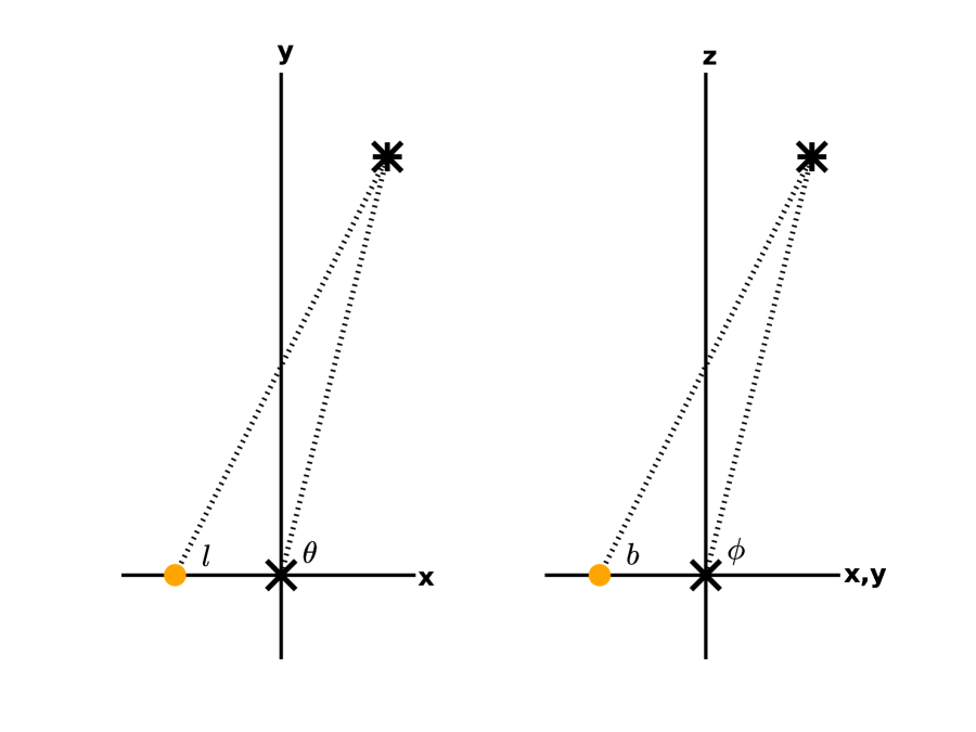
Figure 1: Schematic of the coordinate system. The ‘X’ at the origin indicates the position of the GC. The Sun is represented as the orange dot along the $x$-axis. A star is represented as an asterisk.

To connect these coordinates to the heliocentric galactic system, we assign the Sun a position $(-R_{\odot},0,0)$ and a velocity $(0,v_{\odot},0)$, where $R_{\odot}$ = 8 kpc is the distance of the Sun from the GC (e.g., Bovy et al., 2012) and $v_{\odot}$ is the space velocity of the Sun relative to the GC (Fig. 1). Each star then has a distance $d=((x+R_{\odot})^{2}+y^{2}+z^{2})^{1/2}$ from the Sun and a relative velocity $v_{rel}=(v_{x}^{2}+(v_{y}-v_{\odot})^{2}+v_{z})^{1/2}$. In this system, the galactic longitude $l$ of the star is the angle – measured counter-clockwise in the $x-y$ plane – from a line connecting the Sun to the GC, $l={\rm tan^{-1}}(x~{}{\rm tan}~{}\theta/(x+R_{\odot}))$. The galactic latitude measures the height of the star above the galactic plane, $b={\rm sin^{-1}}(z/d)={\rm sin^{-1}}(r~{}{\rm sin}~{}\phi/d)$. For $r\gg R_{\odot}$, $\theta\approx l$ and $\phi\approx b$.

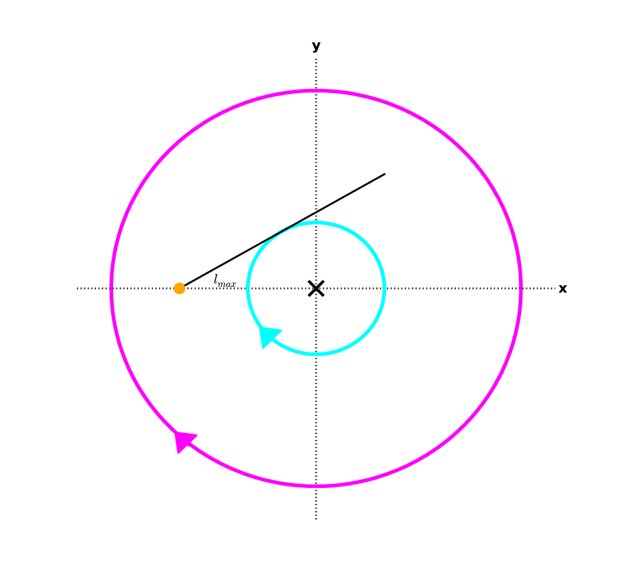
Figure 2: Schematic of stars on circular orbits of the GC. The ‘X’ at the origin indicates the position of the GC. The Sun is represented as the orange dot along the $x$-axis. Stars follow circular orbits around the GC in the direction of the arrows.

Although these coordinate systems are clearly defined, angles in the heliocentric galactic system span a smaller range than in the pure GC system (Fig. 2). For stars with positions $r<R_{\odot}$, the range of $\theta$ ($-\pi$ to $\pi$) is larger than the range of $l$ ($-l_{max}$ to $l_{max}$), where

$$l_{max}={\rm sin^{-1}}(\rho/R_{\odot})~{}.$$ (1)

When $l=l_{max}$, $\theta_{l}={\rm cos}^{-1}(-\rho/R_{\odot})$. For each $l<l_{max}$, there are two values of $\theta$.

We derive the radial velocity $v_{r}$, the tangential velocity $v_{t}$, and the proper motion $\mu$ in the heliocentric frame. For all stars, $v_{rel}^{2}=v_{r}^{2}+v_{t}^{2}$. The radial velocity is

$$v_{r}=v_{x}~{}{\rm cos}~{}l~{}{\rm cos}~{}b+(v_{y}-v_{\odot})~{}{\rm sin}~{}l~{}{\rm cos}~{}b+v_{z}~{}{\rm sin}~{}b~{}.$$ (2)

We separate the tangential velocity into two components, $v_{l}$ and $v_{b}$, where $v_{t}^{2}=v_{l}^{2}+v_{b}^{2}$. The component along the direction of galactic longitude is:

$$v_{l}=-v_{x}~{}{\rm sin}~{}l+(v_{y}-v_{\odot})~{}{\rm cos}~{}l~{}.$$ (3)

The latitude component is

$$v_{b}=-(v_{x}~{}{\rm cos}~{}l+(v_{y}-v_{\odot})~{}{\rm sin}~{}l)~{}{\rm sin}~{}b+v_{z}~{}{\rm cos}~{}b~{}.$$ (4)

For stars with $b\equiv$ 0 and no motion in the $z$-direction, $v_{b}=0$. Although each component of the tangential velocity has a clearly-defined sign convention, we plot the absolute magnitude when we combine the two components into the tangential velocity, $v_{t}=|v_{t}|=(v_{l}^{2}+v_{b}^{2})^{1/2}$.

The standard definition for the proper motion is

$$\mu={v_{t}\over{4.74~{}d}}~{},$$ (5)

where $v_{t}$ is measured in km s^-1 and $d$ is in pc. To set the proper motion in the heliocentric galactic frame, $\mu_{l}=v_{l}/(4.74~{}d)$ and $\mu_{b}=v_{b}/(4.74~{}d)$, where the velocities are in km s^-1. Positive (negative) proper motions are in the direction of increasing (decreasing) $l$ or $b$.

3.2 Simple Trajectories

Within this framework, we consider several simple stellar motions to explore the variation of $v_{r}$ and $v_{t}$ with position in the Galaxy. Most motions are composed of both a circular component and a radial component. Starting with stars following circular orbits around the GC inside and outside the solar circle (§3.2.1), we derive the behavior of $v_{r}$ and $v_{t}$ with $\theta$, $l$, and $b$ for stars with total velocity $v$. In this simple example, we set $z$ = 0 and work in a coordinate system where $r=\rho$. The maximum tangential velocity is then fixed at $v_{t,max}=v+v_{\odot}$; the maximum radial velocity falls with $r$ inside the solar circle and then grows with $r$ outside the solar circle. At large $r$, $v_{r,max}\approx v_{\odot}$. Continuing with stars on purely radial orbits (§3.2.2), we explore motions in the spherical coordinate system appropriate for the bulge and the halo. For stars inside the solar circle, the maximum radial and tangential velocities are $v_{r,max}\approx v$ and $v_{t,max}\approx v+v_{\odot}$. Extrema in $v_{r}$ lie at $l\approx$ 0; stars have maximum $v_{t}$ at $l\approx l_{max}$. Well outside the solar circle, the maximum radial velocity ($v_{r,max}\approx v+v_{\odot}$) is much larger than the maximum tangential velocity ($v_{t,max}\approx v_{\odot}$). At intermediate $r\approx$ 8–20 kpc, there is a smooth transition from small $v_{r,max}$ and large $v_{t,max}$ to large $v_{r,max}$ and small $v_{t,max}$.

3.2.1 Circular Orbital Motion

For stars following simple circular orbits around the GC, $v_{x}=v~{}{\rm sin}~{}\theta$, $v_{y}=-v~{}{\rm cos}~{}\theta$, and $v_{z}$ = 0 (Fig. 2). Although stars in the thin and thick disks have finite vertical distances from the Galactic plane and non-zero motion out of the Galactic plane, we set $z\equiv 0$ and ignore any out-of-plane motion here. Thus, our radial coordinate $r$ is identical to the standard cylindrical coordinate $\rho$. With $\phi=b=0$, the heliocentric radial and tangential velocities are

$$v_{r}=v~{}{\rm sin}~{}\theta~{}{\rm cos}~{}l-(v~{}{\rm cos}~{}\theta+v_{\odot})~{}{\rm sin}~{}l~{}$$ (6)

and

$$v_{t}=-v~{}{\rm sin}~{}\theta~{}{\rm sin}~{}l-(v~{}{\rm cos}~{}\theta+v_{\odot})~{}{\rm cos}~{}l~{}.$$ (7)

In this system, $v_{b}$ = 0 and $v_{t}=v_{l}$. Using trigonmetric identities, we can simplify these to:

$$v_{r}=v~{}{\rm sin}~{}(\theta-l)-v_{\odot}~{}{\rm sin}~{}l~{}$$ (8)

and

$$v_{t}=-v~{}{\rm cos}~{}(\theta-l)-v_{\odot}~{}{\rm cos}~{}l~{}.$$ (9)

For convenience, we can eliminate $\theta$ in the expression for the radial velocity,

$$v_{r}=\left({R_{\odot}\ \over r}v-v_{\odot}\right){\rm sin}~{}l~{}.$$ (10)

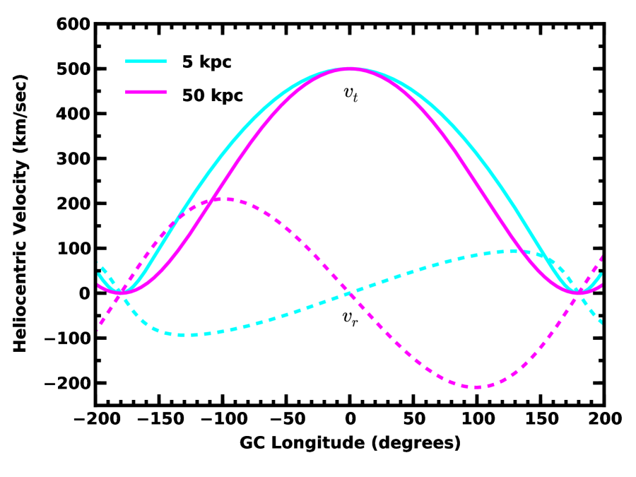
Figure 3: Radial (dashed curves) and tangential (solid curves) velocity for stars with $r$ = 5 kpc (cyan curves) and $r$ = 50 kpc (magenta curves) on circular orbits orbiting the Galaxy with $v$ = 250 km s^-1. In a frame centered on the GC, stars have velocities exactly anti-parallel (parallel) to the motion of the Sun at GC longitude $\theta$ = 0 ($\pm\pi$). At $\theta=0$ ($\theta=\pm\pi$), stars have maximum $|v_{t}|$ and $v_{r}$ = 0 ($v_{r}=v_{t}$ = 0).

Fig. 3 illustrates the variation of $v_{r}$ (dashed curves) and $v_{t}$ (solid curves) with GC longitude for stars with $v$ = 250 km s^-1 and $r$ = 5 kpc (cyan lines) and $r$ = 50 kpc (magenta lines). In this configuration, stars on the opposite side of the Galaxy from the Sun ($\theta=0$) have no net radial velocity and a maximum tangential velocity of $v+v_{\odot}$. For $v_{\odot}$ = 250 km s^-1, $v_{t,max}$ = 500 km s^-1. Stars on the near side of the Galaxy ($\theta=\pm\pi$) have no net radial or tangential velocity. Thus, the minimum tangential velocity is $v_{t,min}$ = 0.

The behavior of $v_{r}$ depends on $r$. For all $r$, $v_{r}=0$ at $\theta=0$ and $\pm\pi$. When $r<R_{\odot}$, maximum positive $v_{r}$ is at $\theta=-\theta_{l}$ ($l=-l_{max}$). Maximum negative $v_{r}$ is at $\theta=+\theta_{l}$. With a maximum radial velocity, $v_{r,max}=\pm(v-v_{\odot}r/R_{\odot})$, the amplitude of the radial velocity variation declines from roughly 250 km s^-1 at $r\approx$ 0 to roughly zero at $r\approx R_{\odot}$. Outside the solar circle, the extrema in $v_{r}$ lie at $l=\pm\pi/2$ ($\theta={\rm cos^{-1}}(-R_{\odot}/r)$). With $v_{r,max}=vR_{\odot}/r-v_{\odot}$, the amplitude of the $v_{r}$ variation grows from zero at $r\approx R_{\odot}$ to $v_{\odot}$ at $r\gg R_{\odot}$. Thus,

$$v_{r,max}=\left\{\begin{array}[]{lll}\pm\left(v-{r\over R_{\odot}}v_{\odot}\right)&&r<R_{\odot}\\ \\ \pm\left({R_{\odot}\over r}v-v_{\odot}\right)&&r\geq R_{\odot}\\ \end{array}\right.$$ (11)

In the heliocentric galactic frame, the variation of $v_{r}$ and $v_{t}$ with $l$ is somewhat different (Fig. 4). For stars inside the solar circle, $v_{t}$ follows an egg-shaped loop with minimum and maximum velocity at $l=0$. Here, $l_{max}$ sets the maximum extent of the loop in galactic longitude. Thus, the ‘egg’ widens at larger $r$, reaching $l_{max}\approx\pm\pi/2$ at $r\approx R_{\odot}$. Outside the solar circle, $v_{t}$ varies sinusoidally with $l$, with maxima of $v$ + $v_{\odot}$ = 500 km s^-1 at $l=\pm\pi$ and a minimum of zero at $l=0$.

The radial velocity also follows simple trajectories. At small $r$, $v_{r}$ varies along a curved line with extrema of $v_{r,max}$ (eq. [11]) at $l_{max}$. As $r$ grows, the curves extend to larger $l$ but have smaller maxima. At large $r$, $v_{r}$ follows a simple sinusoid, with extreme values set by $v_{\odot}$ at $l=\pm\pi/2$ and zero-crossings at $l=0$ and $l=\pm\pi$.

3.2.2 Radial Motion

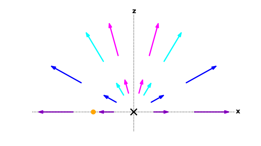
Figure 5: Schematic of stars on radially outflowing orbits from the GC. The ‘X’ at the origin indicates the position of the GC. The Sun is represented as the orange dot along the $x$-axis. Colored arrows indicate velocity vectors for stars with $\phi$ = 0^o (violet), $\phi$ = 30^o (blue), $\phi$ = 60^o (cyan), and $\phi$ = 75^o (magenta). Outside the solar circle (outer set of arrows), all stars move away from the Sun. Inside the solar circle (inner set of arrows), stars with low galactic latitude on the near side of the GC have some component of their motion towards the Sun.

Stars moving radially away from the GC have subtly different behavior. To infer conclusions appropriate for stars in the bulge or the halo, we consider stars with a broad range of GC latitude. In the GC frame, outflowing stars have constant $\phi$ for all $r$ (see Fig. 5). In the heliocentric frame, nearby stars have larger $b$ than more distant stars. For stars with $\phi>0$, $r>\rho$. Thus, distant stars with large $b$ may lie inside the solar circle.

With $v_{x}=v~{}{\rm cos}~{}\theta~{}{\rm cos}~{}\phi$, $v_{y}=v~{}{\rm sin}~{}\theta~{}{\rm cos}~{}\phi$, and $v_{z}=v~{}{\rm sin}~{}\phi$, the heliocentric radial and tangential velocities are

$$v_{r}=v~{}{\rm cos}~{}(\theta-l)~{}{\rm cos}~{}\phi~{}{\rm cos}~{}b-v_{\odot}~{}{\rm sin}~{}l~{}{\rm cos}~{}b+v~{}{\rm sin}~{}\phi~{}{\rm sin}~{}b~{},$$ (12)

$$v_{l}=v~{}{\rm sin}~{}(\theta-l)~{}{\rm cos}~{}\phi-v_{\odot}~{}{\rm cos}~{}l~{},$$ (13)

and

$$v_{b}=-v~{}{\rm cos}~{}(\theta-l)~{}{\rm cos}~{}\phi~{}{\rm sin}~{}b-v_{\odot}~{}{\rm sin}~{}l~{}{\rm sin}~{}b+v~{}{\rm sin}~{}\phi~{}{\rm cos}~{}b~{}.$$ (14)

When stars move radially outward through the Galactic plane, $\phi=b=0$. With $v_{b}=0$, the equations for radial and tangential velocity are then very simple: $v_{r}=v~{}{\rm cos}~{}(\theta-l)-v_{\odot}~{}{\rm sin}~{}l$ and $v_{t}=v_{l}=v~{}{\rm sin}~{}(\theta-l)-v_{\odot}~{}{\rm cos}~{}l$. For stars inside the solar circle, the maximum galactic longitude is $l=l_{max}$.

When $\phi>0$, the variations of $v_{r}$ and $v_{t}$ with $\theta$ and $l$ are more complex. Aside from having a non-zero $v_{b}$, the amplitude of both velocity components declines with cos $\phi$. For stars inside the solar circle, the maximum $l$ scales with $\phi$: $R_{\odot}$ sin $l_{max}$ = $r~{}{\rm cos}~{}\phi$. Thus, stars inside the solar circle at large $\phi$ have a smaller range in $l$ than stars with small $\phi$.

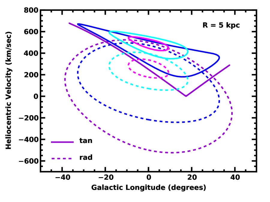
Figure 6: Radial ($v_{r}$, dashed curves) and tangential ($|v_{t}|$, solid curves) velocity as a function of galactic longitude ($l$) for stars at $r$ = 5 kpc and $\phi$ = 0^o (violet), 30^o (blue), 60^o (cyan), and 75^o (magenta) moving radially away from the GC with $v$ = 500 km s^-1.

Fig. 6 shows the variation of $v_{r}$ (dashed curves) and $v_{t}$ (solid curves) as a function of $l$ for stars with $r$ = 5 kpc, $v$ = 500 km s^-1, and $\phi$ = 0^o (violet curves), 30^o (blue curves), 60^o (cyan curves), and 75^o (magenta curves). With $l_{max}\propto\phi$, curves at larger $\phi$ have a smaller extent in $l$. For stars at $r$ = 5 kpc, the maximum galactic latitude is $b\approx$ 30^o–40^o. Both sets of curves follow loops in the $l,v$ plane. For $\phi$ = 0, the $v_{t}$ curve folds back on itself.

When stars lie inside the solar circle, the radial velocity varies symmetrically about an average velocity $v~{}{\rm sin}~{}\phi~{}{\rm sin}~{}b$. This average increases with $\phi$, reaching $v_{r,avg}=v_{\odot}~{}{\rm cos}~{}b+v~{}{\rm sin}~{}b$ at $\phi$ = 90^o. With $b\approx$ 30^o, $v_{r,avg}\approx v_{\odot}$. The amplitude of the $v_{r}$ variation scales with ${\rm cos}~{}\phi$ and thus declines markedly from $\Delta v_{r}\approx v$ to $\Delta v_{r}\approx$ 0 among the sequence of four curves.

The variation of $v_{t}$ with $l$ is not symmetric. At $\phi$ = 0^o, the tangential velocity ranges from a minimum of 0 to a maximum close to $v+v_{\odot}$, roughly 700 km s^-1. At large $\phi$, $v_{t}$ approaches a constant value of roughly $v~{}{\rm cos}~{}b+v_{\odot}~{}{\rm sin}~{}b$ $\approx v$ for $v\gg v_{\odot}$ and $b\approx$ 30^o–40^o.

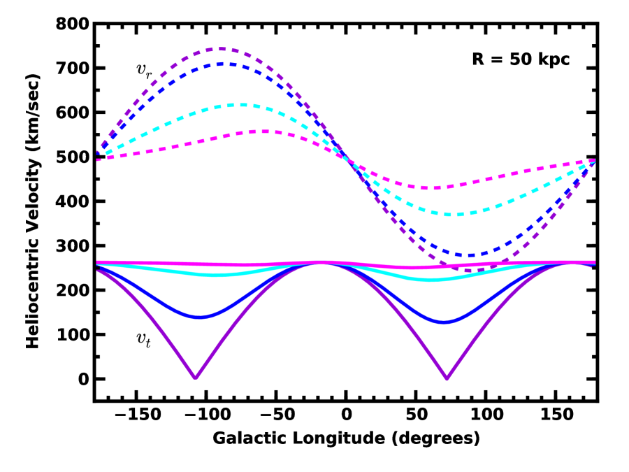
Figure 7: As in Fig. 6 for stars with $r$ = 50 kpc.

Well outside the solar circle ($r$ = 50 kpc), the motions are much simpler (Fig. 7). At large $r$, $v_{r}$ varies roughly sinusoidally with $l$ about an average velocity of $v_{r,avg}\approx v$. The amplitude of this variation decreases with $b$, reaching a constant $v_{r}\approx v$ when $r\gg R_{\odot}$ and $b\approx$ 90^o. Stars reach a minimum (maximum) $v_{r}$ at $l=\pm\pi/2$.

The tangential velocity has a smaller amplitude and different phasing with $l$. At large $b$, the tangential velocity is roughly $v_{\odot}$, a result of reflex solar motion. For stars close to the plane $\phi\approx 0$ and $b\approx$ 0, the tangential velocity consists of two sinusoids with amplitudes of $v$ and $v_{\odot}$ ($v_{t}\approx v_{l}=v~{}{\rm sin}~{}(\theta-l)-v_{\odot}~{}{\rm cos}~{}l$; eq. [13]). Thus, the minimum $v_{t}$ is small and approaches $v_{t}=0$ at $b$ = 0. Because the Sun is offset from the GC, the phase of minimum $v_{t}$ is offset from $\pm\pi/2$. The solar motion and position in the galaxy produce an offset of roughly $-$20^o in longitude.

For stars with 5 kpc $\lesssim r\lesssim$ 50 kpc, there is a smooth transition between the behavior shown in Figs. 6–7. Stars with in-plane distances less than $R_{\odot}$ ($\rho<R_{\odot}$) follow the trajectories in Fig. 6. Stars outside this limit follow the trajectories in Fig. 7.

For an ensemble of stars with $r\approx$ 16 kpc, as an example, stars with $\phi\lesssim\pi/3$ have $\rho\gtrsim R_{\odot}$ and follow the trajectories in Fig. 7. Stars at larger $\phi$ have the closed loop trajectories in Fig. 6.

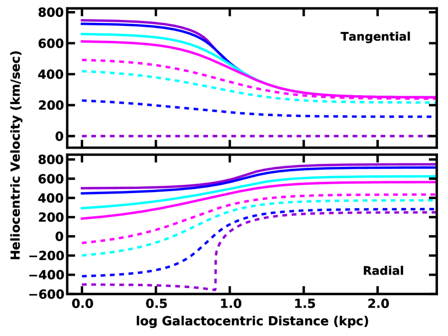
Figure 8: Maximum (solid curves) and minimum (dashed curves) radial velocity (lower panel) and tangential velocity (upper panel) as a function of Galactocentric distance ($r$) for stars at $\phi$ = 0^o (violet), 30^o (blue), 60^o (cyan), and 75^o (magenta) moving radially away from the GC with $v$ = 500 km s^-1.

To illustrate this transition in more detail, Fig. 8 shows the variation of the maximum and minimum radial velocity (lower panel) and tangential velocity (upper panel) as a function of $r$ and $\phi$ for stars on radial orbits with $v$ = +500 km s^-1 relative to the GC. At small $\phi$, the minimum $v_{t}$ is close to zero for all $r$. This minimum increases with $\phi$ until $v_{t}=v_{\odot}$. The maximum $v_{t}$ is roughly constant at 500–750 km s^-1 at small $r$ and then decreases smoothly to $v_{\odot}$ at large $r$.

The extrema in $v_{r}$ have similar trends. Inside the solar circle, stars on the near side of the GC all move towards the Sun and have large negative $v_{r}$. On the far side of the GC, all stars move away from the Sun. Thus, the range in $v_{r}$ is largest for stars inside the solar circle. Because $v_{r}$ scales with cos $\phi$, stars at small (large) $\phi$ have the largest (smallest) range in $v_{r}$.

Outside the solar circle, all stars in this example move away from the Sun. The minimum radial velocity is then always larger than zero, producing the large increase in minimum $v_{r}$ at $r=R_{\odot}$. Somewhat counterintuitively, the maximum $v_{r}$ also grows with $r$. Stars with $r\gtrsim R_{\odot}$ have the largest velocity with respect to the Sun when they move radially outward roughly along the $y$-axis. As $r$ increases, the angle between the $y$-axis and the line-of-sight from the Sun to the star decreases. Thus, the radial component of the relative velocity grows with $r$, reaching $v+v_{\odot}$ when $r\gg R_{\odot}$.

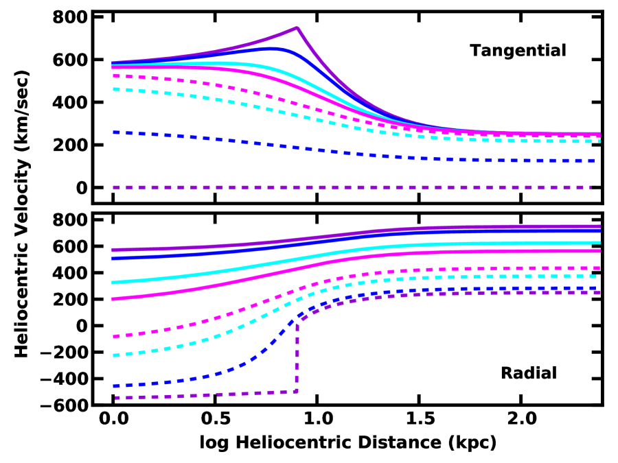
Figure 9: As in Fig. 8 for the heliocentric distance.

Fig. 9 repeats Fig. 8 for heliocentric distance $d$. Aside from a clear discontinuity in the minimum $v_{r}$ for $\phi$ = 0 at $d=R_{\odot}$, the behavior in $v_{r}$ is almost identical to Fig. 8. The minimum $v_{r}$ crosses from negative to positive $v_{r}$ at $d=R_{\odot}$. The maximum $v$ slowly increases to $v+v_{\odot}$ at large $r$. The variation in the minimum $v_{t}$ is also similar, a slowly decreasing function of increasing $r$.

The maximum in the tangential velocity, however, exhibits a clear maximum for stars with $\phi\lesssim$ 30^o at $d$ = 8 kpc. Stars close to the GC produce this maximum. When GC stars move radially outward in the $y$–$z$ plane, their tangential velocity is at a maximum. For $\phi=0$, this peak in $v_{t}$ is a sharp feature. Although still visible for $\phi\approx$ 5^o to 30^o, the feature vanishes for larger $\phi$.

3.3 Summary

Despite the simple stellar motions in these examples, the behavior of $v_{r}$ and $v_{t}$ with $d$, $l$, and $b$ is amazingly rich. For stars inside the solar circle, circular orbital motion and radial outflow produce large maximum tangential velocities, $v_{t,max}\approx v+v_{\odot}$. These maxima occur at distinct galactic longitudes: $l\approx$ 0 for stars orbiting the GC and $l\approx-l_{max}$ for stars moving radially away from the GC. Thus, proper motion measurements offer some promise for distinguishing high velocity stars ejected from the GC from stars on circular orbits around the GC.

Outside the solar circle, circular orbital motion is also distinct from purely radial motion. For stars orbiting the GC, the maximum $v_{t}$ is independent of $r$. However, the maximum tangential velocity of radially outflowing stars gradually declines with $r$ until $v_{t,max}\approx v_{\odot}$. This maximum $v_{t}$ changes little with $l$. For distant stars, orbital motion yields a larger $v_{t,max}$ than radial motion.

Trends of $v_{r}$ with $r$ and $d$ are opposite those of $v_{t}$. Inside the solar circle, stars on circular orbits have smaller and smaller $v_{r}$ at larger and larger $r$. For stars moving radially away from the GC, $v_{r}$ has clear minima and maxima of $\pm v$ at $l\approx\pm l_{max}$. Outside the solar circle, stars on circular orbits have maximum radial velocity $v_{r,max}\approx v_{\odot}$ at large $r$. Stars moving radially away from the GC have much larger maximum $v_{r}$, with $v_{r,max}\approx v+v_{\odot}$. Thus, radial velocity measurements excel at separating distant stars on roughly circular orbits from high velocity stars moving radially outwards from the GC.

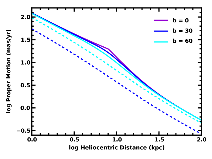
Figure 10: Predicted proper motions for radially outflowing stars as a function of heliocentric distance. The legend indicates the galactic latitude for each curve. Solid curves show the maximum proper motion at each $b$; dashed curves show the minimum proper motion at each $b$.

To conclude this section, we derive predicted proper motions for stars moving radially away from the GC (Fig. 10). Close to the Sun, proper motions are large, roughly 100 milliarcsec yr^-1. The range in proper motions is small (large) for stars at high (small) galactic latitude. At large distances ($d\approx 50-100$ kpc), the maximum proper motion of roughly 1 milliarcsec yr^-1 results from solar reflex motion.

At intermediate distances, there is a small ‘peak’ at $d\approx$ 8 kpc in the trend of $\mu\propto d^{-1}$. Stars inside the solar circle with $l\approx l_{max}$ produce this peak. For $b\approx$ 0^o–10^o, the peak has the largest contrast with the general trend in proper motion (see Fig. 9). At the largest galactic latitudes ($b\gtrsim$ 60^o), the peak fades considerably.

These results demonstrate that radial velocities can isolate high velocity stars from the space motions of typical stars in the Galaxy. Radial velocity measurements succeed at large $d$, where observations can easily separate HVSs or runaways with $v_{r}\gtrsim$ +300 km s^-1 from normal halo stars with $|v_{r}|\lesssim$ 100 km s^-1 (e.g., Brown et al., 2014, and references therein).

Inside the solar circle, proper motion measurements provide a clear path for isolating high velocity stars from bulge and disk stars orbiting the GC. Among B-type stars with $d\lesssim$ 1 kpc, typical proper motions are 10–40 milliarcsec yr^-1 (e.g., de Zeeuw et al., 1999). This motion is a factor of 3–10 times smaller than the predicted motion for nearby HVSs and runaways with space velocities of 500 km s^-1 (Fig. 10). The observed velocity dispersion ($\sigma_{r}\approx$ 100 km s^-1) of stars in the Galactic bulge implies typical proper motions of 1–5 milliarcsec yr^-1 (Tremaine et al., 2002; Soto et al., 2014), smaller than the 10–20 milliarcsec yr^-1 predicted for high velocity HVSs and runaways escaping the inner Galaxy.

For all distances, proper motions alone cannot easily separate ejected stars from indigenous halo stars. The maximum proper motions of typical halo stars with $d\approx$ 1–10 kpc, $\sim$ 30–50 milliarcsec yr^-1 (Kinman et al., 2007, 2012; Bond et al., 2010), are comparable to the likely proper motions of typical ejected stars. We return to this issue in §8.5 with a direct comparison between observations of halo stars and predictions from our numerical simulations.

4 NUMERICAL SIMULATIONS

To explore the space motions of high velocity stars in more detail, we now consider a set of numerical simulations. As in previous papers (Bromley et al., 2006; Kenyon et al., 2008; Bromley et al., 2009), we follow the dynamical evolution of HVSs and runaways throughout their main sequence lifetimes in a realistic Galactic potential. Snapshots of the ensemble yield predictions for the radial distributions of space density, proper motion, and radial velocity. In contrast with previous discussions, we concentrate on observables in the heliocentric frame instead of the Galactocentric frame.

Building a realistic ensemble of HVSs or runaways requires two steps. For each star with main sequence lifetime $t_{ms}$, we generate initial position $\vec{r}_{0}$ and velocity $\vec{v}_{0}$ vectors, an ejection time $t_{ej}$, and an observation time $t_{obs}$, with $t_{ej}\leq t_{obs}\leq t_{ms}$. For a flight time $t_{f}=t_{obs}-t_{ej}$, we integrate the orbit of each star in the Galactic potential and record the final position $\vec{r}_{f}$ and velocity $\vec{v}_{f}$ vectors at $t_{obs}$. Finally, we adopt a position and velocity for the Sun to derive a catalog of $d$, $v_{r}$, $v_{t}$, $\mu_{l}$, and $\mu_{b}$. Analyzing this catalog yields predictions for the observable parameters.

4.1 Gravitational Potential of the Milky Way

As in Kenyon et al. (2008), we adopt a three component model for the Galactic potential $\Phi_{G}$ (for other approaches, see Gnedin et al., 2005; Dehnen et al., 2006; Yu & Madau, 2007):

$$\Phi_{G}=\Phi_{b}+\Phi_{d}+\Phi_{h}~{},$$ (15)

where

$$\Phi_{b}(r)=-GM_{b}/(r+a_{b})~{}$$ (16)

is the potential of the bulge,

$$\Phi_{d}(\rho,z)=-GM_{d}/\sqrt{\rho^{2}+[a_{d}+(z^{2}+b_{d}^{2})^{1/2}]^{2}}$$ (17)

is the potential of the disk, and

$$\Phi_{h}(r)=-GM_{h}\ln(1+r/r_{h})/r$$ (18)

is the potential of the halo (e.g., Hernquist, 1990; Miyamoto & Nagai, 1975; Navarro et al., 1997).

For the bulge and halo, we set $M_{b}=3.76\times 10^{9}M_{\odot}$, $M_{h}=10^{12}M_{\odot}$, $r_{b}$ = 0.1 kpc, and $r_{h}$ = 20 kpc. These parameters match measurements of the mass and velocity dispersion inside 1 kpc and outside 50 kpc (see §2.2 of Kenyon et al., 2008).

To match a circular velocity of 235 km s^-1 at the position of the Sun (e.g., Hogg et al., 2005; Bovy et al., 2012; Reid et al., 2014), we adopt parameters for the disk potential $M_{d}=6\times 10^{10}M_{\odot}$, $a_{d}$ = 2750 kpc, and $b_{d}$ = 0.3 kpc. The complete set of parameters for the bulge, disk, and halo yields a flat rotation curve from 3–50 kpc.

4.2 Initial Conditions

To select $\vec{r}_{0}$ and $\vec{v}_{0}$, we rely on published calculations for HVSs and runaways. For HVSs, we consider a model where a single supermassive black hole at the GC disrupts close binary systems with semimajor axes $a_{bin}$ between $a_{min}$ and $a_{max}$ (Hills, 1988; Kenyon et al., 2008; Sari et al., 2010). Our choice of the minimum semimajor axis $a_{min}$ minimizes the probability of a collision between the two binary components during the encounter with the black hole (Ginsburg & Loeb, 2007; Kenyon et al., 2008). Setting the maximum semimajor axis $a_{max}\approx$ 4 AU limits the number of low velocity ejections which cannot travel more than 10–100 pc from the GC and use a substantial amount of computer time.

4.2.1 Hypervelocity Stars

Numerical simulations of binary encounters with a single black hole demonstrate that the probability of an ejection velocity $v_{ej}$ is a gaussian,

$$p_{H}(v_{ej})\propto e^{(-(v_{ej}-v_{ej,H})^{2}/\sigma_{v}^{2})}~{},$$ (19)

where the average ejection velocity is

$$v_{ej,H}=1760\left(\frac{a_{bin}}{\rm 0.1\ AU}\right)^{-1/2}\left(\frac{M_{1}+M_{2}}{2~{}M_{\odot}}\right)^{1/3}\left(\frac{M_{bh}}{3.5\times 10^{6}~{}M_{\odot}}\right)^{1/6}f_{R}\ \ {\rm km~{}s^{-1}}~{},~{}$$ (20)

and $\sigma_{v}\approx$ 0.2 $v_{ej,H}$ (Bromley et al., 2006). Here $M_{1}$ ($M_{2}$) is the mass of the primary (secondary) star and $M_{bh}$ is the mass of the central black hole. The normalization factor $f_{R}$ depends on $r_{close}$, the distance of closest approach to the black hole:

$$f_{R} = 0.774+(0.0204+(-6.23\times 10^{-4}+(7.62\times 10^{-6}+$$ (21)

$$(-4.24\times 10^{-8}+8.62\times 10^{-11}D)D)D)D)D,$$

where

$$D=D_{0}\left(\frac{r_{close}}{a_{bin}}\right)~{}$$ (22)

and

$$D_{0}=\left[\frac{2M_{bh}}{10^{6}(M_{1}+M_{2})}\right]^{-1/3}.$$ (23)

This factor also sets the probability for an ejection, $P_{ej}$:

$$P_{ej}\approx 1-D/175$$ (24)

for $0\leq D\leq 175$. For $D>175$, $r_{close}\gg a_{bin}$; the binary does not get close enough to the black hole for an ejection and $P_{ej}\equiv 0$.

To establish initial conditions, we select each HVS from a random distribution of $a_{bin}$, $r_{close}$, and $v_{ej}$. The binaries have semimajor axes uniformly distributed in log $a_{bin}$ (e.g., Abt, 1983; Duquennoy & Mayor, 1991; Heacox, 1998). For binaries with $a$ = $a_{max}$, the maximum distance of closest approach is $r_{close,max}=175~{}a_{max}\ /D_{0}$. We adopt a minimum distance of closest approach $r_{close,min}$ = 1 AU. Within this range, the probability of any $r_{close}$ grows linearly with $r$. Choosing two random deviates thus yields $a_{bin}$ and $r_{close}$; $v_{ej,H}$, $D$, and $P_{ej}$ follow from eqs. (20–24). Selecting a third random deviate from a gaussian distribution yields the ejection velocity. Two additional random deviates drawn from a uniform distribution spanning the main sequence lifetime of the star fix $t_{ej}$ and $t_{obs}$. To see whether this combination of parameters results in an ejection, we select a sixth random deviate, $P$, and adopt a minimum ejection velocity $v_{ej,min}$ = 600 km s^-1. Stars with smaller ejection velocities cannot escape the GC (Kenyon et al., 2008). When $P_{ej}\geq P$, $v_{ej}\geq v_{ej,min}$, and $t_{ej}<t_{obs}$, we place the star at a random location on a sphere with a radius of 1.4 pc centered on the GC and assign velocity components appropriate for a radial trajectory from the GC. Failure to satisfy the three inequalities results in a new selection of random numbers.

4.2.2 Runaway Stars

For runaway stars, we consider two analytic models for the ejection velocity. Following Bromley et al. (2009), we assume runaway companions of a supernova have an exponential velocity distribution:

$$p_{S}(v_{ej})\propto e^{-v_{ej}/v_{ej,S}}~{},$$ (25)

where $v_{ej,S}\approx$ 150 km s^-1. For a minimum (maximum) velocity of ejected stars of 20 km s^-1 (400 km s^-1), this distribution roughly matches simulations of binary supernova ejections (Portegies Zwart, 2000).

Predicted velocity distributions for stars ejected dynamically are much steeper (Perets & Subr, 2012). To allow a reasonable number of high velocity ejections, we adopt

$$p_{D}(v_{ej})\propto\left\{\begin{array}[]{lll}v_{ej}^{-3/2}&&v_{ej}\leq v_{ej,D}\\ \\ v_{ej}^{-8/3}&&v_{ej}\geq v_{ej,D}\\ \end{array}\right.$$ (26)

where $v_{ej,D}$= 150 km s^-1 (Perets & Subr, 2012). In our standard calculations, we set a minimum ejection velocity of 20 km s^-1 and a maximum ejection velocity of 800 km s^-1. To improve the accuracy of the statistics for the highest velocity runaways, we perform a second set of simulations with a minimum velocity of 50 km s^-1. Together, these simulations yield a robust picture for the frequency and observable parameters for runaways produced by the dynamical ejection mechanism.

Both of these models yield small production rates for high velocity runaways. To enable more robust comparisons with simulations of HVSs, we consider a ‘toy’ model where the ejection velocity is uniformly distributed between 400 km s^-1 and 600 km s^-1. Thus, we use eqs. (25–26) to derive rates for high velocity runaways and the toy model to understand the galactic distribution of the highest velocity runaways.

Establishing the initial conditions for runaways also requires a set of random deviates. We assume the initial space density of runaways follows the space density of stars in the Galactic disk. Thus, the probability of ejecting a runaway from a cylindrical radius $\rho_{0}$ is

$$p(\rho_{0})\propto\rho_{0}e^{-\rho_{0}/\rho_{s}}~{},$$ (27)

where the scale length is $\rho_{s}$ = 2.4 kpc (Siegel et al., 2002; Bovy & Rix, 2013). We adopt a range for the initial radius, $\rho_{0}$ = 3–30 kpc (Brand & Wouterloot, 2007). Setting the position of the runaway requires two random deviates, one for $\rho_{0}$ and another for the initial longitude in the GC frame. In this approach, the initial height above the Galactic plane is $z=0$.

Once $\rho_{0}$ is known, we choose a random deviate for $v_{ej}$ and two random deviates for the ejection angles (spherical $\theta$ and $\phi$). Adding the velocity from Galactic rotation yields three velocity components. We then choose a final random deviate for $t_{obs}$. In these simulations, ejections occur on time scales much shorter than the lifetime of the ejected star. Thus, $t_{ej}$ = 0.

4.3 Numerical Technique

To integrate the motion of each ejected star through the Galactic potential, we use an adaptive fourth-order integrator with Richardson extrapolation (e.g., Press et al., 1992; Bromley & Kenyon, 2006; Bromley et al., 2009). Starting from an initial position $\vec{r}_{0}$ with velocity $\vec{v}_{0}$, the code integrates the full three-dimensional orbit through the Galaxy, allowing us to track position and velocity as a function of time. We integrate the orbit for a time $t_{f}=t_{obs}-t_{ej}$, which is smaller than the main sequence lifetime of the ejected star. This procedure allows us to integrate millions of orbits fairly rapidly. Several tests demonstrate our approach yields typical errors of 0.01% in position and velocity after 1–10 Gyr of evolution time.

5 REACHING THE HALO

Before analyzing results from the simulations, it is useful to establish the initial conditions which enable ejected stars to reach the Milky Way halo. Stars orbiting the galaxy have a circular velocity $v_{c}^{2}(r)=GM(r)/r$, where $M(r)$ is the mass inside radius $r$. For our adopted Milky Way potential, $v_{c}\approx$ 235 km s^-1 for disk stars with $r\approx$ 3–30 kpc. To reach the halo, ejected stars must have a total velocity comparable to the escape velocity, $v_{esc}(r)$. To set $v_{esc}(r)$, we calculate the velocity required for particles starting from radius $r$ to reach $r$ = 250 kpc with zero velocity. For HVSs ejected at $r$ = 1.4 pc, $v_{esc}\approx$ 913 km s^-1. At $r\approx$ 3–30 kpc, $v_{esc}(r)\approx$ 537 $(r/{\rm 10~{}kpc})^{-0.19}$ km s^-1. Brown et al. (2014) quote a more accurate, polynomial approximation to $v_{esc}$ which is valid over a larger range of Galactocentric distances.

With the definitions in §4.2.1, many HVSs ejected from the GC reach the outer halo. In our simulations, roughly 18% of HVSs have initial velocities larger than $v_{esc}$. Another 6% have ejection velocities, $v_{0}\approx$ 850–913 km s^-1, sufficient to reach $r\approx$ 60–100 kpc. For these speeds, typical travel times to reach the halo are 100–250 Myr (see also Brown et al., 2014). If most HVS ejections occur roughly in the middle of the main sequence lifetime, stars with $t_{ms}\gtrsim$ 200–500 Myr escape the Galaxy as main sequence stars (e.g., Bromley et al., 2006; Kenyon et al., 2008; Rossi et al., 2013).

Among the bound population of HVSs, most lie close to the GC. Roughly 60% of ejected stars have $v_{ej}$ = 600–750 km s^-1 and maximum distances of 1 kpc from the GC. With their low Galactic latitudes, $b\lesssim$ 7^o, detecting this population requires infrared surveys. Another 5% have $v_{ej}$ = 755–780 kms; these stars have maximum distances of 5–20 kpc from the GC. Compared to the 18% of unbound HVSs, the population of bound HVSs near the solar circle makes up a small fraction of all ejected stars.

Despite starting far from the GC, it is hard for runaways to reach the outer halo. In the supernova ejection model, the maximum ejection velocity of 400 km s^-1 is smaller than the escape velocity of 660 km s^-1 (430 km s^-1) at $r$ = 3 kpc (30 kpc). Although the maximum velocity in the dynamical ejection model, 800 km s^-1, exceeds $v_{esc}$ at all locations in the disk, few runaways achieve such large ejection velocities. Typical velocities are smaller than 400 km s^-1. Thus, runaways need a boost from Galactic rotation to reach the halo (see also Bromley et al., 2009).

To quantify the fraction of runaways which can escape the disk and reach the outer halo, we consider the initial velocity of an ejected star with rotational velocity $\vec{v}_{c}$ and ejection velocity $\vec{v}_{ej}$. The angles between the two velocity vectors are $\alpha$ (in the Galactic plane) and $\beta$ (out of the plane). The initial velocity of the star is then

$$v_{0}^{2}=v_{c}^{2}+v_{ej}^{2}+2v_{c}v_{ej}{\rm cos}~{}\alpha~{}{\rm cos}~{}\beta~{}.$$ (28)

For any $v_{ej}$, stars ejected along the direction of Galactic rotation ($\alpha=\beta=0$) have the maximum initial velocity, $v_{0}=v_{c}+v_{ej}$. These stars have the best chance to reach the outer part of the Galaxy. Stars ejected in the opposite direction ($\alpha=-\pi$, $\beta$ = 0) have the smallest initial velocity, $v_{0}=v_{c}-v_{ej}$, and the worst chance to reach the outer Galaxy. When stars are ejected perpendicular to the disk ($\beta$ = $\pi$/2), they have an intermediate velocity, $v_{0}=(v_{c}^{2}+v_{ej}^{2})^{1/2}$, and a modest chance to reach the halo. At other angles, $v_{0}$ has a constant value when $\alpha=-\beta$ (sin $(\alpha+\beta)$ = 0), which defines a circle in the $\alpha-\beta$ plane.

To calculate the fraction of runaways which can reach $r\gtrsim$ 60 kpc, we derive the allowed range of $\alpha$ and $\beta$ for runaways with ejection velocity $v_{ej}$ starting from distance $r$ from the GC. Integrating over the appropriate probability distributions for $v_{ej}$ (eqs. [25–26]), the initial position (eq. [27]), and the ejection angles yields the total fraction $f$ of runaways with initial distance $r$ that reach $r\gtrsim$ 60 kpc. To illustrate the difficulty of reaching the Galactic halo, we calculate $f$ for all runaways and those with maximum $b\gtrsim$ 30^o.

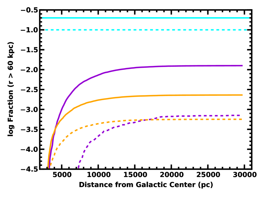
Figure 11: Cumulative fraction of stars with final Galactocentric distances, $d\gtrsim$ 60 kpc, as a function of their initial position in the disk for supernova-induced runaways (violet curves) and dynamically generated runaways (orange curves). Solid lines plot results for all stars; dashed lines show results for halo stars with $|b|\geq$ 30^o. Cyan lines show the fraction of HVSs ejected from the GC which reach the halo (solid line: all $b$; dashed line: $|b|\geq$ 30^o).

This exercise demonstrates that few runaways reach the outer Galaxy (Fig. 11). Roughly 1% of all supernova-induced runaways travel beyond 60 kpc (solid violet curve). Stars with initial positions $r\lesssim$ 10 kpc contribute nearly all of the ejected stars. Within this group, less than 10% (0.1% of all runaways) reach $d\gtrsim$ 60 kpc with $|b|\gtrsim$ 30^o. Although dynamical ejections into the outer Galaxy are more rare ($\sim$ 0.3% of the total population), dynamical ejections into the outer halo are as frequent as supernova-induced ejections, $\sim$ 0.06% of all runaways.

The larger maximum ejection velocity in the dynamical model accounts for these differences. Most runaways are ejected at 3–5 kpc, where the escape velocity is large. With a maximum $v_{ej}$ of 400 km s^-1, supernova-induced runaways require the maximum boost from Galactic rotation to reach the outer Galaxy. Sacrificing some of this boost to eject stars into the halo keeps stars from reaching the outer Galaxy. Few of these high $b$ runaways reach the outer halo. Dynamically ejected stars with ejection velocities of 600–800 km s^-1 require little boost from Galactic rotation. These stars easily reach the outer halo. Compared to the supernova model, however, the dynamical model yields a smaller fraction of stars with high velocities. The lack of high velocity stars compensates for the relative ease of reaching the halo, resulting in comparable fractions of high velocity halo stars with $r\gtrsim$ 60 kpc in both models.

If the production rates for HVSs and both types of runaways are comparable, this analysis predicts that HVSs dominate the population of high velocity stars in the outer halo. For every high speed runaway generated by a supernova or a dynamical interaction among massive stars, there should be roughly 100 HVSs. We will re-consider this conclusion in §8.6 when we examine predicted production rates for each mechanism.

6 COMPLETE SAMPLES OF STARS

All ejection models yield populations of bound and unbound stars (Bromley et al., 2006; Kenyon et al., 2008; Bromley et al., 2009). To explore the properties of both populations, we consider simulations of 1 $M_{\odot}$ and 3 $M_{\odot}$ stars. Calculations with long-lived solar-type stars provide a sample of bound stars in the solar neighborhood and a sample of unbound stars with a broad range of distances. While current facilities can probe the bound population, most unbound stars are too distant and too faint for detailed study. Although simulations with shorter-lived, more luminous 3 $M_{\odot}$ stars yield a smaller sample of bound stars, the population of unbound stars is well-matched to the sensitivity of GAIA and large ground-based optical telescopes. These two sets of simulations allow us to derive general predictions for the bound and unbound populations.

The numerical simulations of the motions of HVSs and runaways through the Galaxy yield ensembles of $10^{6}-10^{7}$ stars with final positions $\vec{r}_{f}$ and velocities $\vec{v}_{f}$ relative to the GC. These data represent a snapshot of all ejected stars still on the main sequence. The HVSs fill a spherical volume from the GC out to roughly 1 Mpc (34 Mpc) for 3 $M_{\odot}$ (1 $M_{\odot}$) stars. Although runaways are more concentrated towards the Galactic disk (e.g., Bromley et al., 2009), a few reach Galactocentric distances of $\sim$ 300 kpc (3 $M_{\odot}$) to 7 Mpc (1 $M_{\odot}$). To put these results in perspective, the modern magnitude-limited surveys described in §7 can probe 1 $M_{\odot}$ (3 $M_{\odot}$) stars to $d$ = 10 kpc (100 kpc).

To derive heliocentric observables for each star in a snapshot, we set the Sun at a position $(-R_{\odot},0,0)$ with velocity $(0,v_{\odot},0)$ relative to the GC. We adopt $R_{\odot}$ = 8 kpc and $v_{\odot}$ = 235 km s^-1 (e.g., Bovy et al., 2012) and divide each ensemble into five distance bins, $d\leq$ 10 kpc, 10 kpc $<d\leq$ 20 kpc, 20 kpc $<d\leq$ 40 kpc, 40 kpc $<d\leq$ 80 kpc, and 80 kpc $<d\leq$ 160 kpc. Tables 1–2 list the median $v_{med}$, first and third quartile $v_{q1}$ and $v_{q3}$, average $v_{avg}$, and standard deviation for the radial ($\sigma_{r}$) and tangential ($\sigma_{t}$) velocities in each simulation. Table 3 summarizes statistics for the proper motion. For runaways produced by dynamical interactions, we quote results for simulations with a minimum ejection velocity of 50 km s^-1. Velocity distributions for calculations with a smaller ejection velocity of 20 km s^-1 are fairly similar to those for supernova-induced runaways.

In the next subsections, we examine several broad trends in the variation of $\mu$ and $v_{r}$ with $d$, $l$, and $b$. After discussing predicted distributions of stars in the $d-\mu$ (§6.1) and $d-v_{r}$ (§6.2) planes, we describe predicted histograms for $v_{r}$ and $\mu$ in well-defined distances bins and for the complete ensemble of stars in each simulation (§6.3). To isolate how observables depend on Galactic coordinates, we then discuss the distribution of stars in the $l-\mu$ plane for specific ranges of Galactic latitude (§6.4). This section concludes with a brief summary of the major results (§6.5).

6.1 Ejected Stars in the $d-\mu$ Plane

To investigate the distribution of stars as a function of $\mu$ and $d$, we construct a density diagram. For stars with $|b|\geq$ 30^o, we (i) divide the log $d$–log $\mu$ plane into bins spaced by 0.01 in log $d$ and log $\mu$, (ii) count the number of stars in each bin, and (iii) plot the relative number in a contour diagram. In each diagram, bright red represents the largest density; dark blue the smallest density. The full range in relative density varies from a factor of 5–10 for 1 $M_{\odot}$ runaways to a factor of 50–500 for 1–3 $M_{\odot}$ HVSs.

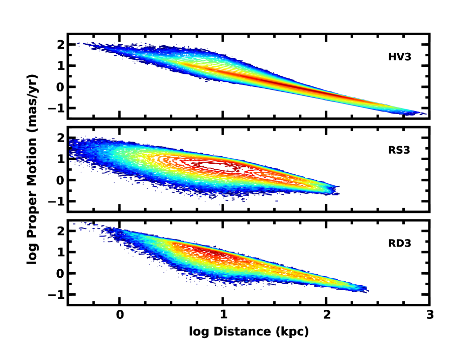
Figure 12: Predicted density distributions of 3 $M_{\odot}$ HVSs and runaways with $|b|\geq$ 30^o in the $\mu-d$ plane. In each panel, the density scale is logarithmic with a minimum of 0.0 (displayed as dark blue). The maximum of the density (displayed as bright red) varies from 2.7 (HV3) to 1.7 (RS3) to 1.4 (RD3). Upper panel: most 3 $M_{\odot}$ HVSs lie along the linear $\mu(d)$ relation expected for reflex solar motion. HVSs ejected out the Galactic poles lead to a small concentration above this relation at $d\approx$ 10 kpc. Middle panel: compared to HVSs, 3 $M_{\odot}$ runaways ejected during a supernova show much more scatter about the linear $\mu(d)$ relation for reflex solar motion. At large distances, the bimodal proper motion distribution of 3 $M_{\odot}$ runaways mirrors Galactic rotation. Lower panel: 3 $M_{\odot}$ runaways ejected from dynamical interactions among massive stars follow the linear $\mu(d)$ relation and display a bimodal proper motion distribution at large $d$. Due to their larger ejection velocities, some runaways reach larger distances. Runaways in the Galactic anti-center produce the ensemble of nearby stars with very small proper motions.

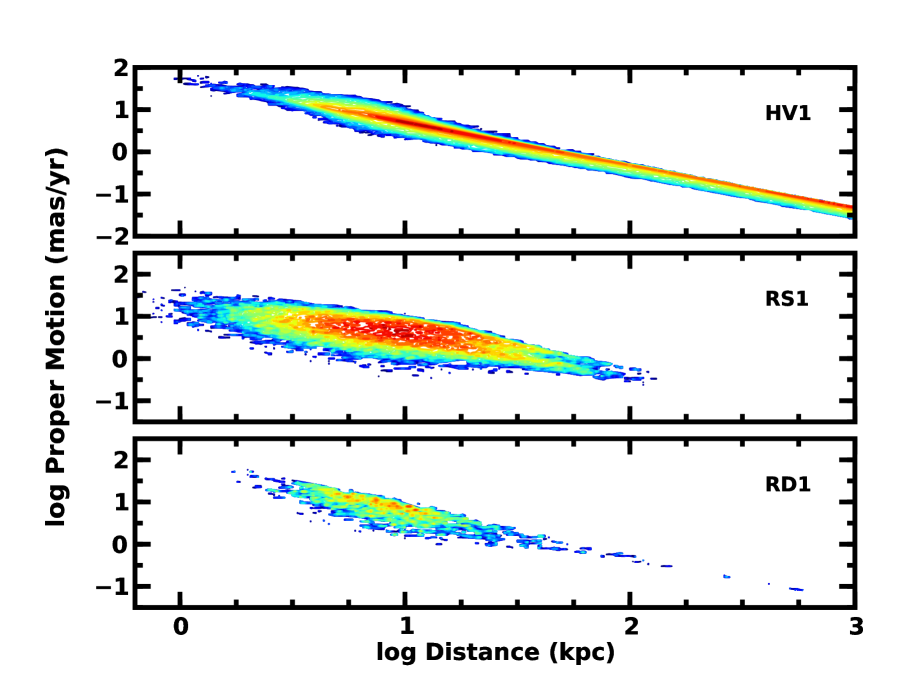
Figure 13: As in Fig. 12 for 1 $M_{\odot}$ stars. The maximum of the density is 1.8 (HV1), 1.0 (RS1), or 0.7 (RD1). Upper panel: the distribution of 1 $M_{\odot}$ HVSs extends to large $d$, with two density maxima at 10 kpc and at 2–3 Mpc. Middle panel: Most supernova-induced runaways have $d\approx$ 10 kpc; a few reach $d\gtrsim$ 80 kpc. Lower panel: Few dynamically-generated runaways reach high Galactic latitude. Most of these have $d\lesssim$ 10 kpc; a few reach $d\approx$ 100–200 kpc.

Fig. 12 shows predicted density distributions for 3 $M_{\odot}$ HVSs and runaways. Fig. 13 plots predictions for 1 $M_{\odot}$ stars. The HVS results assume stars ejected from equal mass binaries (1 $M_{\odot}$: $a_{bin}$ = 0.032–4 AU, $t_{ms}$ = 10 Gyr; 3 $M_{\odot}$: $a_{bin}$ = 0.115–4 AU, $t_{ms}$ = 350 Myr). For the runaway simulations, we adopt minimum ejection velocities of 20 km s^-1 (supernova ejections) or 50 km s^-1 (dynamical ejections). Eliminating the lower velocity dynamical ejections artificially enhances the density at large proper motions relative to small proper motions. This enhancement provides a clearer picture of the relative frequency of the highest velocity runaways.

These results demonstrate that nearly all of the proper motions for 3 $M_{\odot}$ HVSs result from reflex solar motion (Fig. 12, upper panel). Most HVSs fall close to the line

$$\mu=49.6\left({d\over{\rm 1~{}kpc}}\right)~{}{\rm milliarcsec~{}yr^{-1}}~{}.$$ (29)

At fixed $d$, stars with smaller $\mu$ have smaller $b$ (see also Fig. 10). Along the locus, the number of 3 $M_{\odot}$ HVSs peaks at $d\approx$ 50 kpc.

Above the $\mu(d)$ locus, there is a cloud of stars with $d\lesssim$ 10–20 kpc and $\mu\lesssim$ 100 milliarcsec yr^-1. This group of mostly bound HVSs lies at all $b$ in the direction of the GC. Stars ejected along the $z$-axis produce this clump of high proper motion stars (see Fig. 10).

Although runaways generally follow the $\mu(d)$ relation expected for reflex solar motion, the distribution about this relation is much more diffuse than for HVSs (Fig. 12, middle and lower panels). Galactic rotation produces this fuzziness. In HVS ejections, the distribution of ejection velocities is gaussian; the position of a star along the $\mu(d)$ relation is a simple function of this ejection velocity and the flight time. In runaway ejections, the ejection velocity consists of Galactic rotation plus a random velocity with a random angle relative to Galactic rotation. This randomness creates a much larger dispersion of space velocities and much larger dispersion about the simple $\mu(d)$ relation.

For $d\approx$ 20–100 kpc, galactic rotation also produces twin peaks in the density at fixed distance. Separated by roughly 0.3 in log $\mu$, these twin density maxima are very prominent in the ensemble of supernova-induced runaways (middle panel) and less prominent among the dynamically generated runaways (lower panel). For runaways in the Galactic anti-center, the rotational component of their motion is parallel to the Sun’s motion. These stars lie in the low proper motion peak. Distant runaways in the direction of the GC are beyond the GC; the rotational component of their space motion is anti-parallel to the Sun’s motion. These stars produce the high proper motion peak. Nearby indigenous disk stars in the direction of the GC have rotational motions parallel to the Sun, eliminating the double-peaked aspect of the proper motion distribution.

The larger maximum velocities from dynamical ejections blur the double-peaked distributions of proper motions identified in runaways from supernovae (Fig. 12, lower panel). Despite the diffuse nature of the contour diagram, Galactic rotation is clearly visible at 20–50 kpc. As with HVSs and supernova-induced runaways, the width of the proper motion distribution narrows with increasing distance.

Results for 1 $M_{\odot}$ HVSs and runaways are similar (Fig. 13). The HVSs closely follow the linear $\mu(d)$ relation out to $d$ = 30 Mpc (Fig. 13, upper panel). The density of 1 $M_{\odot}$ HVSs has two clear maxima at $d\approx$ 10 kpc and $d\approx$ 2–3 Mpc. Stars at high $b$ closely follow the line (red contour); stars at $b\approx$ 30^o occupy the blue contour below the line. At $d\approx$ 10 kpc, there is a group of stars with large $\mu$ above the red contour. High velocity ejections along the Galactic poles produce this collection of large proper motion stars (see also Fig. 10).

Despite their lower frequency, 1 $M_{\odot}$ runaways also clearly follow the linear $\mu(d)$ relation expected for solar reflex motion. Aside from having a shape similar to the contours for the 3 $M_{\odot}$ runaways, the contours for 1 $M_{\odot}$ runaways extend to slightly larger distances due to their longer main sequence lifetimes.

The number and location of density peaks for HVSs in Fig. 12–13 depend solely on stellar lifetime (see also Bromley et al., 2006; Kenyon et al., 2008). For ejected stars with infinite lifetimes, the space density $n$ is a simple power-law with distance from the GC, $n\propto r^{-2}$. Thus, the total number of HVSs grows monotonically with distance. However, real HVSs have finite lifetimes. The total number falls at distances where the travel time exceeds the main sequence lfetime. For 1 $M_{\odot}$ (3 $M_{\odot}$) HVSs with ejection velocities drawn from eq. (20), lifetimes of 10 Gyr (350 Myr) result in peaks at 2–3 Mpc (50 kpc). The second peak in the density of 1 $M_{\odot}$ stars results from bound stars with orbital periods smaller than the main sequence lifetime. Continuous ejection of relatively low velocity HVSs over 10 Gyr produces a large concentration of bound 1 $M_{\odot}$ HVSs with $d\lesssim$ 20 kpc. The short lifetimes of 3 $M_{\odot}$ HVSs preclude a significant concentration of nearby HVSs.

The space density of stars in the disk sets the density of runaways in these diagrams. For stars with an exponential distribution of ejection velocities, unbound stars are very rare (§5). Thus, most stars in the diagram are bound to the Galaxy. For bound stars at $|b|>$ 30^o, the final in-plane distance from the GC, $\rho_{f}$, is similar to the initial distance, $\rho_{0}$. The space density of these stars follows the initial density, which is concentrated towards the GC. As a result, most stars have $d\lesssim$ 10–20 kpc.

In both diagrams, the dynamical and supernova ejection scenarios produce an ensemble of stars at $d\approx$ 10 kpc with smaller proper motions than the locus of stars with solar reflex motion. Within this group, stars with the smallest $\mu$ are concentrated towards small $b$ at a variety of Galactic longitudes $l\approx\pm$100^o–280^o where the tangential velocity reaches a minimum. Some of these stars have large ejection velocities parallel to the Sun’s trajectory (see Fig. 7). Others have modest ejection velocities perpendicular the plane, which enable them to reach large $b$ but not escape the Galaxy (see Fig. 4).

6.2 Ejected Stars in the $d$-$v_{r}$ Plane

To explore the variation of radial velocity with distance, we examine another density diagram. As in the previous section, we (i) select stars with $|b|\geq$ 30^o, (ii) divide the log $d$–$v_{r}$ plane into bins spaced by 0.01 in log $d$ and 20 km s^-1 in $v_{r}$, and (iii) count the number of stars in each bin. In the diagrams, bright red represents the largest density; dark blue the smallest density. The range in density varies from a factor of 50 for 1 $M_{\odot}$ runaways to a factor of 300 for 3 $M_{\odot}$ HVSs and runaways.

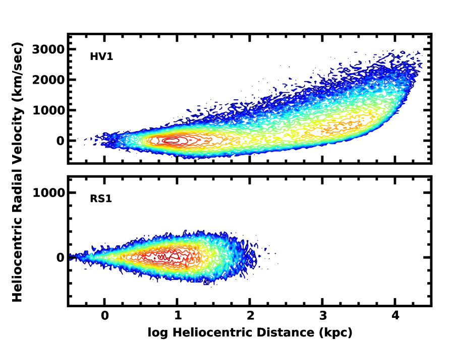
Figure 14: Predicted density distributions of 1 $M_{\odot}$ HVSs and supernova-induced runaways with $|b|\geq$ 30^o in the $v_{r}-d$ plane. In each panel, the density scale is logarithmic with a minimum of 0.0 (displayed as dark blue) and a maximum (displayed as bright red) of 2.1 (HV1) or 1.7 (RS1). Upper panel: bound 1 $M_{\odot}$ HVSs lie within a band from 5–50 kpc symmetric about median $v_{r}$ = 0 km s^-1. Beyond this locus, unbound HVSs produce a secondary peak at $d\approx$ 1–5 Mpc. Lower panel: compared to HVSs, 1 $M_{\odot}$ runaways ejected during a supernova have a much more symmetric distribution of $v_{r}$ with $d$. All supernova-induced runaways are bound; most lie within 10–20 kpc and have small median $v_{r}$ and $\sigma_{r}$. None reach $d\gtrsim$ 100 kpc.

HVSs and runaways from supernovae show a remarkable diversity in the relative density of 1 $M_{\odot}$ stars as a function of $v_{r}$ and $d$ (Fig. 14). Close to the Sun ($d\lesssim$ 1–3 kpc), the relatively few HVSs and runaways have fairly symmetric velocity distributions around a median $v_{r}\approx$ 0 km s^-1. At moderate distances ($d\approx$ 3–20 kpc), the spread in radial velocity grows smoothly with distance. Although HVSs have a much larger spread in radial velocity (see also Table 1), both groups have a clear peak in the relative number of stars at $d\approx$ 10 kpc and $v_{r}\approx$ 0–100 km s^-1.

For stars at large distances ($d\gtrsim$ 20 kpc), the velocity distributions of HVSs and supernova-induced runaways differ dramatically. With their modest maximum ejection velocities, few runaways reach the outer Galaxy (§5; Fig. 11). For $d\gtrsim$ 20 kpc, the density of runaways drops significantly and falls very close to zero at $d\approx$ 100 kpc. Despite the steep fall in relative density, the median velocity and the spread in radial velocity are roughly constant with distance (Table 1).

The properties of distant HVSs provide a clear contrast with distant runaways. For HVSs, the median radial velocity and the spread in the radial velocity grow with distance. The maximum radial velocity increases from roughly 1000 km s^-1 at $d\approx$ 10 kpc to 3000 km s^-1 at $d\approx$ 10–20 Mpc. Although the relative density of HVSs falls from 20 kpc to 300 kpc, the relative density displays a clear secondary peak at $d\approx$ 2 Mpc and $v_{r}\approx$ 400–500 km s^-1. Beyond 5 Mpc, the density slowly falls and reaches roughly zero at $d\approx$ 20 Mpc.

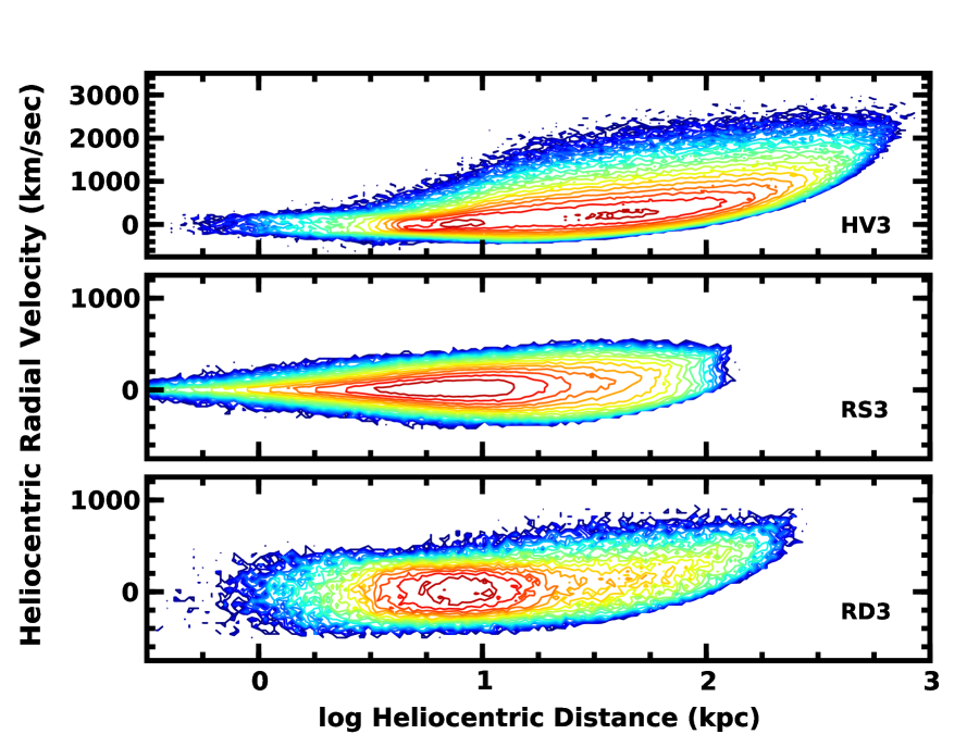
Figure 15: As in Fig. 14 for 3 $M_{\odot}$ ejected stars. The maximum density is 2.5 (HV3), 2.6 (RS3), or 1.9 (RD3). Upper panel: most bound 3 $M_{\odot}$ HVSs lie within the narrow red band where the median $v_{r}$ increases with distance at $d\approx$ 10–100 kpc. Above this locus, unbound HVSs within the green and blue contours have large $v_{r}$. Middle panel: compared to HVSs, 3 $M_{\odot}$ runaways ejected during a supernova have a much more symmetric distribution of $v_{r}$ with $d$. All supernova-induced runaways are bound; most lie within 10–20 kpc and have small median $v_{r}$ and $\sigma_{r}$. None reach $d\gtrsim$ 100 kpc. Lower panel: 3 $M_{\odot}$ runaways ejected from dynamical interactions among massive stars have median $v_{r}\approx$ 0 km s^-1 and dispersion $\sigma_{r}\approx$ 100–150 km s^-1 at $d\lesssim$ 10–20 kpc. Nearly all of these runaways are bound. At larger distances, a few unbound stars reach $d\gtrsim$ 50–100 kpc with large $v_{r}$.

The distributions of 3 $M_{\odot}$ runaways are similar to those of 1 $M_{\odot}$ runaways (Fig. 15). In the middle panel, supernova-induced runaways show a clear increase in relative density from $d\approx$ 300 pc to $d\approx$ 10 kpc. Within this range of distances, the spread in the radial velocity grows smoothly with distance; the median $v_{r}$ is close to zero. Beyond this peak, the relative density drops to zero at $d\approx$ 100 kpc. Among the more distant stars, the maximum $v_{r}$ is roughly constant with distance; the minimum $v_{r}$ grows slowly with distance.

Dynamically-generated runaways yield similar results. When we adopt a minimum $v_{ej}$ = 20 km s^-1 for dynamically-generated runaways, the distribution is nearly indistinguishable from the middle panel of Fig. 15. Increasing the minimum $v_{ej}$ to 50 km s^-1 removes the ensemble of low velocity stars from the diagram, reducing the density and increasing the spread in $v_{r}$ for nearby stars (Fig. 15, lower panel). Despite this difference, dynamically generated runaways still display a clear peak in relative density at $d\approx$ 10 kpc. Around this peak, stars have a median $v_{r}$ close to zero and a spread of $\pm$500 km s^-1 (Table 1).

Because the dynamical model yields a maximum $v_{ej}\approx$ 800 km s^-1, a few runaways reach larger distances and have larger radial velocities than supernova-induced runaways. Despite this difference, very few runaways are unbound (§5).

Although 3 $M_{\odot}$ HVSs have a nearly identical distribution of ejection velocities as 1 $M_{\odot}$ HVSs, the density distributions in the $d$–$v_{r}$ plane show several clear differences. The primary peak in the density lies at somewhat smaller distances, at $\sim$ 8 kpc instead of $\sim$ 10 kpc. The secondary peak falls at much smaller distances, $\sim$ 50 kpc instead of a few Mpc. The drop in density at large distances is much more rapid, falling to zero just inside 1 Mpc instead of reaching to 30 Mpc.

These trends have simple physical explanations (Bromley et al., 2006; Kenyon et al., 2008). For our adopted MW potential and HVS parameters, roughly 10% of ejected stars have velocities large enough to reach 10–20 kpc but too small to travel beyond 60–100 kpc. Typical travel times of 100–400 Myr for these bound stars are a significant fraction of the main sequence lifetime of a 3 $M_{\odot}$ star, but are much smaller than the lifetime of a 1 $M_{\odot}$ star. Bound stars with long lifetimes have median velocities close to zero and modest velocity dispersions of 100–200 km s^-1. However, many bound stars with short lifetimes reach $d\approx$ 30–60 kpc and evolve off the main sequence before returning to the solar circle. Thus, there is a large deficit of bound, massive stars with negative radial velocity. For 3 $M_{\odot}$ stars, this deficit leads to a median $v_{r}$ larger than zero and a larger velocity dispersion than 1 $M_{\odot}$ HVSs (see also Table 1).

Among unbound stars, finite stellar lifetimes are also responsible for trends in $v_{r}$ with distance. Stars with larger ejection velocities reach larger distances; the median $v_{r}$ and dispersion in $v_{r}$ thus increase with $d$. Longer lifetimes also enable stars to reach larger $d$. With a factor of 30 longer lifetime, the 1 $M_{\odot}$ stars reach 30 times larger distances than 3 $M_{\odot}$ stars (30 Mpc instead of 1 Mpc).

The initial velocity distributions of HVSs and runaways produce the stark differences in Figs. 14–15. Among runaways ejected from 3–30 kpc in the Galactic disk, nearly all have modest ejection velocities and remain bound to the Galaxy (§5). Bound stars with modest ejection velocities reach maximum distances of roughly 100 kpc before falling back into the Galaxy. The small fraction of runaways which reach the halo have typical $d\approx$ 10 kpc and $v_{r}\lesssim$ 100–150 km s^-1.

6.3 Radial Velocity and Proper Motion Histograms

The density plots in Figs. 12–15 demonstrate the rich behavior in the predicted $\mu(d)$ and $v_{r}(d)$ as a function of initial conditions and stellar properties. To focus on predictions for large ensembles of HVSs and runaways, we now consider the frequency distributions of $v_{r}$ and $\mu$ for Galactic halo stars ($|b|\geq$ 30^o) in a discrete set of distance bins. In these diagrams, color encodes distance (violet: $d\leq$ 10 kpc, blue: 10 kpc $<d\leq$ 20 kpc, green: 20 kpc $<d\leq$ 40 kpc, and orange: 40 kpc $<d\leq$ 80 kpc). Tables 1–3 summarize statistics for $\mu$, $v_{r}$, and $v_{t}$ in each distance bin.

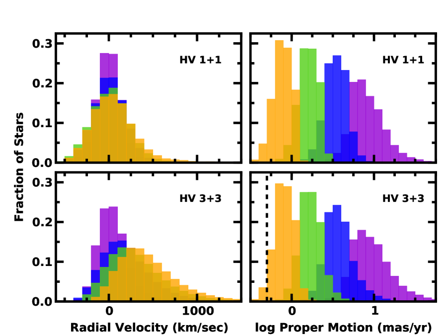
Figure 16: Predicted distributions of radial velocity (left panels) and proper motion (right panels) velocity for HVSs produced from 1 $M_{\odot}$ + 1 $M_{\odot}$ binaries (upper panels) and from 3 $M_{\odot}$ + 3 $M_{\odot}$ binaries (lower panels) with Galactic latitude $|b|>$ 30^o and distances $d<$ 10 kpc (violet histograms), 10 kpc $<d<$ 20 kpc (blue histograms), 20 kpc $<d<$ 40 kpc (green histograms), and 40 kpc $<d<$ 80 kpc (orange histograms). Dashed lines in the right panels indicate the 3$\sigma$ GAIA detection limit for stars with $g\lesssim$ 20 (Lindegren, 2010). The median radial velocity (proper motion) grows (falls) with increasing distance. More massive HVSs have larger radial velocities.

Fig. 16 shows the distributions of $v_{r}$ (left panels) and $\mu$ (right panels) for 1 $M_{\odot}$ (upper panels) and 3 $M_{\odot}$ (lower panels) HVSs. The trends of radial velocity with stellar mass and distance follow the correlations in §6.2 (see also Bromley et al., 2006; Kenyon et al., 2008). For 3 $M_{\odot}$ stars, the median radial velocity grows with increasing distance. Among the more distant stars, there is a large tail of very high velocity stars with $v_{r}\gtrsim$ 1000 km s^-1. As distance decreases, a smaller and smaller fraction of stars have high velocities. In the nearby sample with $d\leq$ 10 kpc, nearly all stars have $v_{r}\lesssim$ 500 km s^-1.

For 1 $M_{\odot}$ stars, the trend of increasing median velocity with increasing distance is much weaker (Table 1). For all $d$, the velocity dispersion and inter-quartile range are smaller. Although the typical maximum velocity is similar, a much smaller fraction of stars has $v_{r}\gtrsim$ 1000 km s^-1.

The distributions of proper motion and tangential velocity reverse the trends of the radial velocity (Tables 2–3; Fig. 16, right panels). Distant HVSs moving radially away from the GC have small transverse components of their space motion, leading to small tangential velocities and small proper motions. As the distance decreases, the angle between the line-of-sight and the velocity vector for an HVS grows, leading to larger and larger tangential velocities. With $\mu\propto d^{-1}$, nearby HVSs have much larger proper motions than more distant HVSs (see also Fig. 9). Although geometry requires that the maximum $v_{r}$ exceed the maximum $v_{t}$, some nearby HVSs have $v_{t}\approx$ 400–600 km s^-1 and $\mu\approx$ 30 milliarcsec yr^-1.

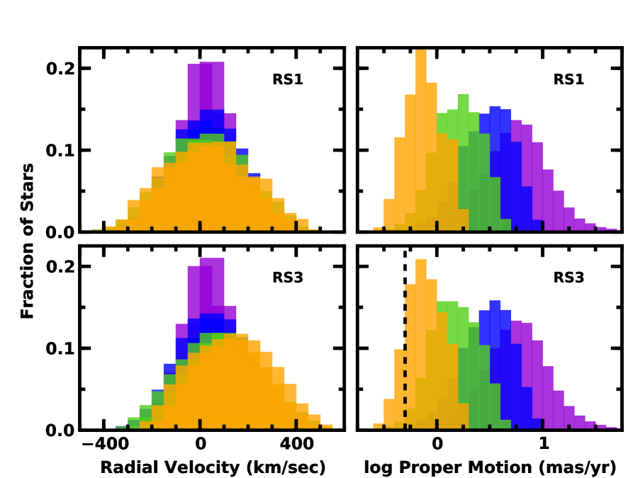
Figure 17: As in Fig. 16 for 1 $M_{\odot}$ runaway stars (upper panels) and 3 $M_{\odot}$ runaway stars. The stars have an exponential distribution of ejection velocities (eq. [25]). As with HVSs, the median radial velocity (proper motion) grows (falls) with increasing distance.

Trends in the radial velocity distributions for supernova-induced runaways follow those of the HVSs (Fig. 17; Table 1). More distant runaways have a larger median radial velocity and a larger tail to very large radial velocity (see also Bromley et al., 2009). At fixed distance, however, the average and median velocities of runaways are much smaller than those of HVSs. Typically, runaways are 100–500 km s^-1 slower than HVSs, with velocity dispersions less than half the dispersions of HVSs.

Differences between the radial velocity distributions for HVSs and runaways in the snapshots reflect the initial distribution of ejection velocities. As summarized in §5, more than 20% of the HVSs ejected with initial velocities exceeding 600 km s^-1 reach the halo. Most HVSs that reach the halo are unbound. The fastest runaways receive a boost from Galactic rotation (eq. [28]); they all lie in the Galactic plane (see also Bromley et al., 2009). Many fewer runaways reach the halo; nearly all of these have much smaller space velocities than HVSs. As a result, runaways in the halo have smaller median radial velocities and a larger fraction of bound stars than HVSs.

At similar distances, the proper motion distribution of both types of runaways is broader than that of HVSs (Fig. 17, right panels). As with HVSs, nearby runaways have larger tangential velocities than more distant runaways. However, galactic rotation produces a double-peaked distribution of proper motion for runaways at fixed distance (Fig. 12–13). In an ensemble of stars with a broad range of distances, the double-peaked character of the distribution smears out into a single broad peak. Among stars with a smaller range of distances, the double-peaked proper motion distribution is prominent.

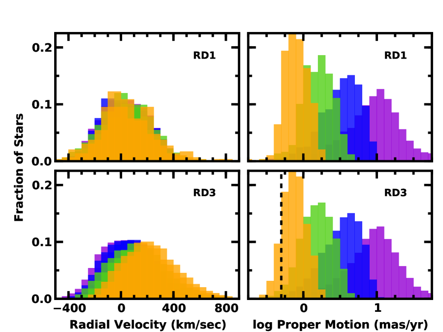
Figure 18: As in Fig. 16 for runaways with a power-law distribution of ejection velocities (eq. [26]).

The distributions of $v_{r}$ and $\mu$ for runaways produced from dynamical ejections have the same features as supernova-induced runaways. The median radial velocity grows with distance (Fig. 18, left panels). Although dynamical ejections produce a smaller fraction of high velocity runaways, the largest ejection velocities exceed those produced from the supernova mechanism (Table 1). For calculations with a minimum ejection velocity of 20 km s^-1, dynamical ejections yield average and median velocities 5%–10% smaller than supernova-induced runaways. In simulations with a minimum ejection velocity of 50 km s^-1, the inter-quartile ranges and standard deviations for dynamical ejections lie between those of HVSs and runaways produced in supernovae.

The larger maximum velocities from dynamical ejections shift the peaks of the proper motion distributions to larger values (Fig. 18, right panels; see also Table 3). These peaks are also somewhat broader than those for other ejected stars. As with HVSs and supernova-induced runaways, the width of the proper motion distribution narrows with increasing distance.

For 3 $M_{\odot}$ HVSs and runaways, GAIA can detect the typical proper motion in the $d$ = 40–80 kpc bins (dashed lines in Figs. 16–18). To establish this conclusion, we use the predicted rms errors of roughly 0.16 milliarcsec yr^-1 for stars with $g\approx$ 20 (Lindegren, 2010). Observed proper motions of 0.50 milliarcsec yr^-1 should then be detectable at the 3$\sigma$ level. Although solar-type stars with $g\approx$ 20 have $d\approx$ 10 kpc, 3 $M_{\odot}$ B-type stars with $g\approx$ 20 have $d\approx$ 100 kpc (see also §7). Thus, reliable distances and proper motions from GAIA can test these predicted proper motion distributions.

As we described in §6.1, proper motion distributions for HVSs and runaways are very sensitive to stellar lifetime. Long-lived unbound stars travel great distances from the Galaxy; shorter-lived stars evolve off the main sequence before leaving the Galaxy. Long-lived bound stars generate fairly symmetric distributions around the GC; shorter-lived stars have more asymmetric distributions.

At high galactic latitude ($|b|\geq$ 30^o), HVSs provide the most extreme examples of this behavior (Fig. 19, top panels). With lifetimes of 10 Gyr, unbound 1 $M_{\odot}$ stars reach maximum distances of roughly 30 Mpc from the GC. These unbound stars produce the prominent peak at $\mu\approx$ 0.01–0.05 milliarcsec yr^-1 in the upper left panel of Fig. 19. Bound 1 $M_{\odot}$ stars have maximum distances of roughly 60 kpc; they orbit the GC with periods of 700 Myr or less. Smaller distances result in much larger proper motions. These stars comprise the smaller peak in the upper left histogram at $\mu\approx$ 1–10 milliarcsec yr^-1.

Among all HVS ejections, bound stars outnumber unbound stars by roughly 4:1 (§5). Outside the Galactic plane ($|b|\geq$ 30^o), however, unbound stars dominate. Thus, the peak of unbound stars at small $\mu$ is larger than the peak of bound stars at large $\mu$.

Despite having similar ejection velocities as low mass HVSs, massive unbound HVSs do not live long enough to reach large distances from the GC. With typical maximum distances of roughly 1 Mpc, the smallest proper motions of unbound 3 $M_{\odot}$ HVSs are roughly a factor of 30 larger than those of unbound 1 $M_{\odot}$ HVSs. Although there are a few massive HVSs with $\mu\approx$ 0.03–0.10 milliarcsec yr^-1, most have $\mu\gtrsim$ 0.1 milliarcsec yr^-1. These stars lie within the peak at $\mu\approx$ 1 milliarcsec yr^-1 in the upper right panel of Fig. 19.

At $|b|\geq$ 30^o, bound 3 $M_{\odot}$ HVSs have a much larger range in proper motion. Marginally bound stars reach large distances from the GC, $r\approx$ 40–60 kpc. Before they turn around and return to the GC, these stars evolve off the main sequence. This group has fairly small proper motion $\mu\approx$ 1 milliarcsec yr^-1. Among the much larger group of bound stars that reach small distances, $r\lesssim$ 10–20 kpc, some have $|b|\gtrsim$ 30^o. These have large proper motions, $\mu\gtrsim$ 10 milliarcsec yr^-1. In between, stars with $d\approx$ 20–40 kpc fill in the histogram at $\mu\approx$ 1–10 milliarcsec yr^-1.

These general conclusions apply to both types of runaways. Among stars ejected by dynamical processes, a few have ejection velocities of 600–900 km s^-1 and can reach large distances from the Galaxy. Low mass stars in this group are still on the main sequence at $d\gtrsim$ 1 Mpc; these stars produce a long tail in the proper motion distribution at $\mu\approx$ 0.01–0.5 milliarcsec yr^-1 (Fig. 19, lower left panel). More massive stars cannot reach these distances while on the main sequence; 3 $M_{\odot}$ unbound stars produce a small shoulder in the distribution at $\mu\approx$ 0.1–0.3 milliarcsec yr^-1 (Fig. 19, upper right panel).

For all masses, the dynamical ejection process yields a large population of bound, relatively nearby stars. Typical proper motions are $\mu\approx$ 1–20 milliarcsec yr^-1. Nearly all stars in the peaks of both histograms are bound stars.

With much lower maximum ejection velocities, stars ejected during a supernova are almost always bound to Galaxy. Among 1–3 $M_{\odot}$ stars, most are nearby. Few have $\mu\lesssim$ 0.5 milliarcsec yr^-1. These stars simply produce a single peak in the histogram at $\mu\approx$ 3–4 milliarcsec yr^-1.

At large $\mu$, the shapes of all of the histograms are fairly similar. For all of our snapshots, nearby stars with high velocity are rare. Most runaways with $d\lesssim$ 1 kpc have small velocities and modest proper motions. HVSs fill a much larger volume of the Galaxy and have much smaller space densities. Thus, the frequency of ejected stars with $\mu\gtrsim$ 10 milliarcsec yr^-1 falls sharply and reaches zero at $\mu\approx$ 100 milliarcsec yr^-1.

6.4 Proper Motion in Galactic Coordinates

To conclude our analysis of complete snapshots of ejected stars, we focus on the variation of proper motion with $l$ and $b$. After separating stars into four galactic latitude bins equally spaced in $|{\rm sin}~{}b|$, we divide the $l$–$\mu$ plane into a set of bins spaced by 0.01 in log $\mu$ and 1^o in $l$. As with the $d$–$\mu$ and $d$–$v_{r}$ diagrams in §6.1–6.2, we plot the relative density of stars in each bin as a contour diagram where bright red represents the largest density and dark blue represents the smallest density. The range in density varies from a factor of 5–10 for 1 $M_{\odot}$ runaways to a factor of 50–500 for 1–3 $M_{\odot}$ HVSs.

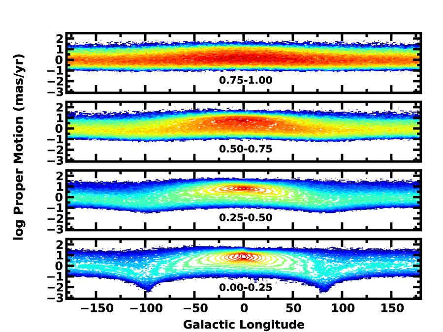
Figure 20: Predicted density distributions for 3 $M_{\odot}$ HVSs as a function of $l$ and $b$. The range in $|{\rm sin}~{}b|$ is listed in each panel. The density scale is logarithmic with a minimum of 0.0 (displayed as dark blue). The maximum of the density (displayed as bright red) is 3.6 (lowermost panel), 2.6 (lower middle panel), 1.6 (upper middle panel), and 1.4 (uppermost panel). At all $l$, there is at least a two order of magnitude range in $\mu$. Towards the Galactic anti-center, the median proper motion is small, $\mu\approx$ 1 milliarcsec yr^-1. Ejections along the Galactic poles produce a dense concentration of HVSs with large $\mu$ towards the GC at all $b$. The concentration weakens with increasing $b$. Close to the Galactic plane, solar reflex motion produces clear minima in $\mu$ for radially outflowing stars at $l\approx$ $-$100^o and $+80$^o.

Fig. 20 shows a set of four contour diagrams for 3 $M_{\odot}$ HVSs. At all $b$, HVSs have a broad range of proper motion between 0.1 milliarcsec yr^-1 and 30 milliarcsec yr^-1. Outside the GC region, the typical proper motion is $\mu\approx$ 1 milliarcsec yr^-1. Towards the GC, there is a strong concentration of stars with large proper motion, $\mu\approx$ 10–100 milliarcsec yr^-1. This concentration is strongest at low Galactic latitude and weakens considerably at larger $b$.

In the Galactic plane (Fig. 20, lowermost panel), the variation of $\mu$ with $l$ for HVSs shows a clear signature from the Sun’s orbit around the GC (see eq. [13]; compare with Fig. 7). The plot shows clear minima in $\mu$ at $l$ = $-$100^o and at $l$ = $+$80^o. The Sun’s (i) spatial offset from the GC and (ii) orbit around the GC produces the lack of mirror symmetry in the minima (see also Fig. 7). At somewhat larger $b$ (middle two panels), the amplitude of the variation is visible but suppressed. Towards the Galactic poles (uppermost panel), the Sun’s position and orbital velocity have no impact on the tangential velocity. Thus, the variation disappears.

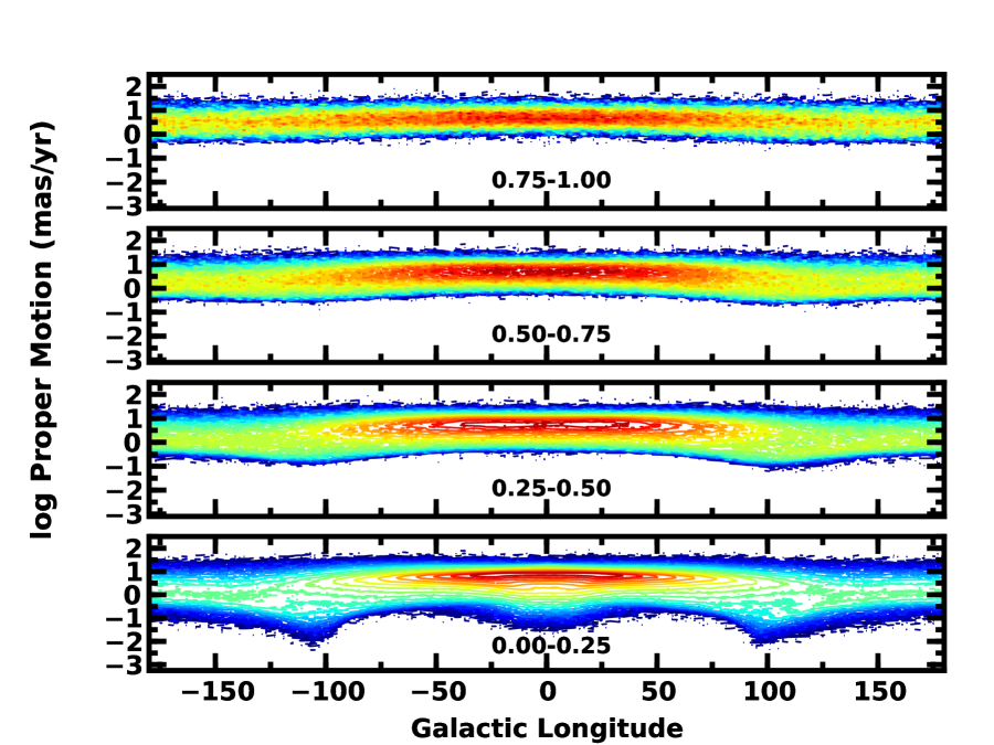
Figure 21: As in Fig. 20 for supernova-induced runaways. The maximum of the density is 3.6 (lowermost panel), 2.1 (lower middle panel), 1.6 (upper middle panel), and 1.2 (uppermost panel). Stars ejected from the disk are heavily concentrated to the GC, which yields runaways with large $\mu$ towards the GC at all $b$. As with HVSs, the concentration weakens with increasing $b$. Close to the Galactic plane, solar reflex motion produces clear minima in $\mu$ at $l\approx$ $\pm$100 ^o. Stars orbiting inside the solar circle produce the distinct minimum in $\mu$ towards the GC.

Contour diagrams for supernova-induced runaways display identical features (Fig. 21). Runaways have somewhat larger proper motions than HVSs, with a typical $\mu\approx$ 3 milliarcsec yr^-1 and a typical range of 0.3–30 milliarcsec yr^-1. Although HVSs have larger space velocities, their much larger distances result in smaller proper motions.

As with HVSs, the contour diagrams change systematically with Galactic latitude. In the Galactic plane (Fig. 21, lowermost panel), runaways display a large concentration of high proper motion stars towards the GC. At larger $b$, this concentration weakens and spreads to a broader range of Galactic longitude. High velocity runaways outside the solar circle but close to the Galactic plane also show clear minima in $\mu$ at $l\approx$ $-$110^o and $+$100^o. As noted for high velocity HVS in Fig. 20, these minima are a clear signature of solar rotation around the GC and the solar offset from the GC (see Fig. 7). This signal gradually diminishes with increasing $b$.

A clear minimum in $\mu$ at $l\approx$ 0 and $|{\rm sin}~{}b|<$ 0.25 (Fig. 21, lowermost panel) distinguishes supernova-induced runaways from HVSs. For stars inside the solar circle, this feature is the signature of stars rotating in the Galactic disk (see Fig. 4). Inside the solar circle, the tangential velocities of stars orbiting the GC lie in an egg-shaped locus with $v_{t,max}\approx$ 2 $v_{\odot}$ and $v_{t,min}\approx$ 0. The lower edge of this egg produces the distinct minimum in $\mu$ at $l\approx$ 0.

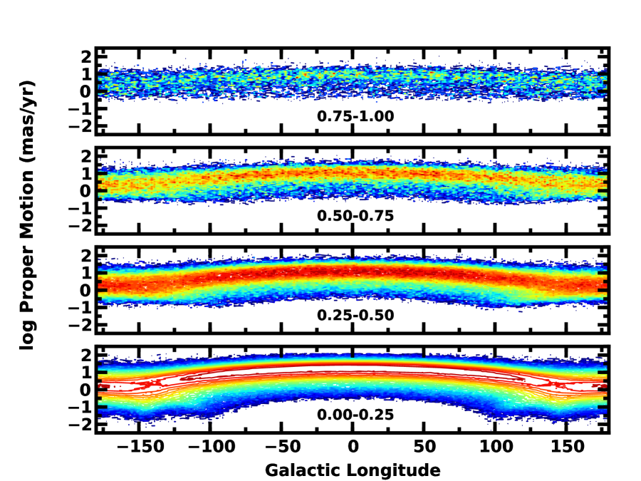
Figure 22: As in Fig. 20 for dynamically-produced runaways with a minimum ejection velocity of 50 km s^-1. The maximum of the density is 2.5 (lowermost panel), 1.4 (lower middle panel), 1.0 (upper middle panel), and 0.8 (uppermost panel). As with supernova induced runaways, runaways with large $\mu$ are heavily concentrated towards the GC at all $b$. The concentration weakens with increasing $b$. Close to the Galactic plane, solar reflex motion produces clear minima in $\mu$ at $l\approx$ $\pm$100 ^o. With a minimum ejection velocity of 50 km s^-1, stars orbiting inside the solar circle at $l\approx$ 0^o never have a distinct minimum in $\mu$ towards the GC. However, small ejection velocities produce a deeper minimum in $\mu$ towards the Galactic anti-center.

Dynamical runaways with a minimum velocity of 20 km s^-1 produce distributions of $\mu(l,b)$ nearly identical to the distributions for supernova-induced runaways in Fig 21. Calculations with a minimum velocity of 50 km s^-1 yield dramatically different results (Fig. 22). Although (i) the typical range in $\mu(b)$, (ii) the heavy concentration of stars towards the GC, and (iii) the clear minima in $\mu$ at $l\approx\pm$ 100^o observed for dynamical runaways are similar to results for supernova-induced runaways, there is (i) a clear lack of stars with very small $\mu$ at $l\approx$ 0^o and (ii) a broad minimum of stars with very small $\mu$ at $l\approx\pm$150–180^o.

The higher minimum ejection velocity in these calculations produces both features. Stars on unperturbed orbits around the GC produce the distinct minimum in $\mu$ at $l\approx$ 0^o. Setting a high minimum ejection velocity in our calculations produces ensembles of stars with modest tangential velocities and proper motions at $l\approx$ 0^o, eliminating the pronounced minimum in $\mu$ at $l$ = 0^o in Fig. 21. This high minimum ejection velocity also tends to place stars onto orbits with modest eccentricity. Stars originating inside the solar circle – where the stellar density is large – then spend some time outside the solar circle – where the stellar density is small. This behavior increases the density of stars with small proper motion in the direction of the Galactic anti-center, where the tangential velocity is very small (see Fig. 3).

6.5 Summary

Analyzing the complete sample of stars in simulations of HVSs and runaways leads to several clear results.

• Ejections produce a broad range in $v_{r}$ (0–1000 km s^-1), $v_{t}$ (0–600 km s^-1), and $\mu$ (0.01–100 milliarcsec yr^-1). HVSs have the largest velocities and proper motions (Figs. 12–15).

• For distant stars, radial velocities separate unbound stars from bound stars (Figs. 14–15 and Figs. 16–18).

• For nearby stars, proper motions distinguish between unbound stars and bound stars on radial or circular orbits. However, nearby unbound stars are relatively rare compared to nearby bound stars (Figs. 12–13 and Fig. 19).

• Unbound runaways retain memory of their original orbital velocity around the GC. At large distances and high Galactic latitudes, the double-peaked proper motion distribution of runaways distinguishes them from stars on radial orbits (Figs. 12–13).

• In the Galactic plane, HVSs and runaways have clear, distinctive minima in $\mu(l)$ at $l\approx\pm$100^o (Figs. 20–22).

• Concentrations of high proper motion stars towards the GC are a unique signature of HVSs ejected from the GC or runaways ejected from the inner galaxy (Figs. 20–22).

• GAIA can detect predicted proper motions of B-type HVSs and runaways with $d\lesssim$ 100 kpc (Figs. 16–18).

These results clearly demonstrate the ability of radial velocity measurements to distinguish the highest velocity HVSs and runaways from indigenous halo stars (see also Brown et al., 2005, 2006; Bromley et al., 2006; Kenyon et al., 2008; Silva & Napiwotzki, 2011; Brown et al., 2014, and references therein). For HVSs and runaways with $d\gtrsim$ 50–100 kpc, the median radial velocity, 500–600 km s^-1, and radial velocity dispersion, $\sigma_{r}\approx$ 200–400 km s^-1, are very different from the population of halo stars with median $v_{r}$ close to zero and $\sigma_{r}\approx$ 100–110 km s^-1. Thus, radial velocity surveys easily separate the highest velocity HVSs and runaways from indigenous halo stars.

Among stars with intermediate distances, $d\approx$ 20–40 kpc, proper motions can distinguish runaways from indigenous halo stars. For runaway stars with a small range of distances, galactic rotation produces a clearly double-peaked distribution of proper motions. With little or no rotation about the GC (e.g., Bond et al., 2010), halo stars should have a broad, single-peaked distribution. Because HVSs are ejected on purely radial orbits, their distribution of proper motions should resemble the halo distribution.

Among nearby halo stars with $d\lesssim$ 10 kpc and $|b|\gtrsim$ 30^o, kinematic data do not offer a simple path for identifying ejected stars. The velocity dispersions, $\sigma_{r}\approx$ 100–175 km s^-1, of nearby HVSs and runaways are comparable to the typical velocity dispersion of halo stars (e.g., Brown et al., 2014, and references therein). Thus, it is not possible to use $v_{r}$ to distinguish nearby HVSs and runaways from halo stars. Although the dispersions in $v_{t}$ for nearby HVSs and runaways are small, the median $v_{t}\approx$ 250 km s^-1 for HVSs and dynamically generated runaways is much larger than the roughly 150 km s^-1 dispersion in $v_{t}$ expected for indigenous halo stars. Because nearby HVSs and runaways are rare, their proper motions are fairly similar to the proper motions of nearby halo stars.

As with radial velocities, obvious outliers in proper motion are promising candidates for ejected stars. Our simulations yield maximum proper motions of 100 milliarcsec yr^-1 for stars with $d\lesssim$ 1–2 kpc. Along any line-of-sight, however, such high proper motion stars comprise only 0.01–0.1% of the complete population of ejected stars. Thus, high proper motion outliers should be very rare.

7 DISTANCE LIMITED SAMPLES OF STARS

To construct a clear set of testable predictions from the simulations, we now focus on distance-limited (magnitude-limited) samples of 1 $M_{\odot}$ and 3 $M_{\odot}$ HVSs and runaways. Based on the expected sensitivity of GAIA, we establish a magnitude limit. For convenience, we base this limit on the SDSS $g$ magnitude (e.g., Brown et al., 2014). Using stellar evolution models, we convert the magnitude limit into a distance limit $d_{max}$. Finally, we draw stars with $d\leq d_{max}$ from the complete simulations of HVSs and runaways. These catalogs allow us to predict distributions of $v_{r}$ and $\mu$ for comparison with observations.

For 1–3 $M_{\odot}$ stars with $g\lesssim$ 20, GAIA observations should yield proper motions with rms errors of 0.16 milliarcsec yr^-1 (e.g., Lindegren, 2010; Lindegren et al., 2012). Brighter stars have much smaller errors, roughly 0.08 milliarcsec yr^-1 for $g\approx$ 19 and 0.05 milliarcsec yr^-1 for $g\approx$ 18. Because GAIA should detect proper motions of roughly 0.15–0.5 milliarcsec yr^-1 for stars with $g\approx$ 18–20, we set a magnitude limit of $g$ = 20.

To convert this magnitude limit to a distance limit, we derive absolute magnitudes $M_{g}$ from the Padova stellar evolution models. For solar metallicity (Z = 0.019; e.g., Bressan et al., 2012), $M_{g}$(1 $M_{\odot}$) = 5.1 at $t$ = 5 Gyr and $M_{g}$(3 $M_{\odot}$) = 0.17 at $t$ = 172.5 Myr. These ages are half of the adopted main-sequence lifetimes of 10 Gyr and 345 Myr for these stars (e.g., Bressan et al., 2012). These magnitudes then yield distance limits of $d_{max}$ = 9.55 kpc (92.5 kpc) for an ensemble of middle-aged 1 $M_{\odot}$ (3 $M_{\odot}$) stars. We round these limits to 10 kpc for 1 $M_{\odot}$ stars and 100 kpc for 3 $M_{\odot}$ stars.

In this first exploration of distance-limited samples of HVSs and runaways from our simulations, we ignore several aspects of stellar evolution and Galactic structure. We assume stars are unreddened, which is reasonable for halo stars at high galactic latitude (e.g., Schlegel et al., 1998). Although metallicity has a small impact ($\sim$ 0.1 mag) on $M_{g}$ for 3 $M_{\odot}$ stars, these stars brighten by roughly 1 mag during their main sequence lifetime (Bressan et al., 2012). For ensembles of 1 $M_{\odot}$ stars, metallicity and stellar evolution produce a 0.5–0.75 mag spread in $M_{g}$ (Bressan et al., 2012). Thus, $g$ = 20 3 $M_{\odot}$ (1 $M_{\odot}$) main sequence stars with a range of ages and metallicities have a 10% to 20% range in distances. This range is small compared to the obvious trends in $v_{r}$, $v_{t}$, and $\mu$ with $d$, $l$, and $b$ derived from our simulations. Thus, we can safely adopt uniform samples of identical stars with no range in age or metallicity.

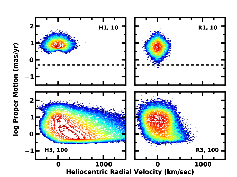
Figure 23: Predicted density plots in the $v_{r}$-$\mu$ plane for distance-limited samples of HVSs (left panels) and runaways (right panels). The legend codifies the stellar mass (1 $M_{\odot}$ or 3 $M_{\odot}$) and the distance (10 kpc or 100 kpc). Magnitude-limited samples of 1 $M_{\odot}$ stars (top panels) have a small predicted range for $v_{r}$ and $\mu$. All predicted proper motions lie above the 3$\sigma$ GAIA detection limit for stars u with $g\lesssim$ 20 (dashed line; Lindegren, 2010). Magnitude-limited samples of 3 $M_{\odot}$ stars (lower panels) cover a broader range in $v_{r}$ and $\mu$.

Fig. 23 compares predicted density distributions in the $v_{r}$–$\mu$ plane for distance-limited samples of HVSs (left panels) and runaways (right panels). Contours for 1 $M_{\odot}$ (3 $M_{\odot}$) stars are in the upper (lower) panels. For simplicity, we show results for 1 $M_{\odot}$ supernova-induced runaways and for 3 $M_{\odot}$ dynamically generated runaways. Density distributions for other runaway models have similar morphology to those shown in this diagram.

The loci for 1 $M_{\odot}$ HVSs and runaways are fairly similar. Compared to the set of contours for 3 $M_{\odot}$ stars in the lower panels, both ensembles have a limited extent in radial velocity and proper motion, with $v_{r}\approx$ $-$250 km s^-1 to $+$250 km s^-1 and $\mu\approx$ 1–30 milliarcsec yr^-1. The HVS contours have a broader extent in $v_{r}$ and a much narrower extent in $\mu$ than the contours for the runaways. The median proper motion of roughly 6 milliarcsec yr^-1 for 1 $M_{\odot}$ HVSs is somewhat larger than the median proper motion of 5 milliarcsec yr^-1 for 1 $M_{\odot}$ runaways.

The ensemble of 3 $M_{\odot}$ ejected stars fills a much larger portion of $v_{r}$–$\mu$ space. HVSs and runaways have a large concentration of bound stars with median $v_{r}$ close to 0 km s^-1 and median proper motion of roughly 3–10 milliarcsec yr^-1. Both populations contain a group of unbound stars with larger $v_{r}$ and smaller $\mu$. Among the runaways, this group produces a modest ‘tail’ in the distribution which comprises less than 0.1% of the entire population. For HVSs, however, the tail extends to $v_{r}\approx$ 1000–1500 km s^-1 and contains more than half of the ensemble. Nearly all of the unbound HVSs have small proper motion, $\mu\lesssim$ 1 milliarcsec yr^-1.

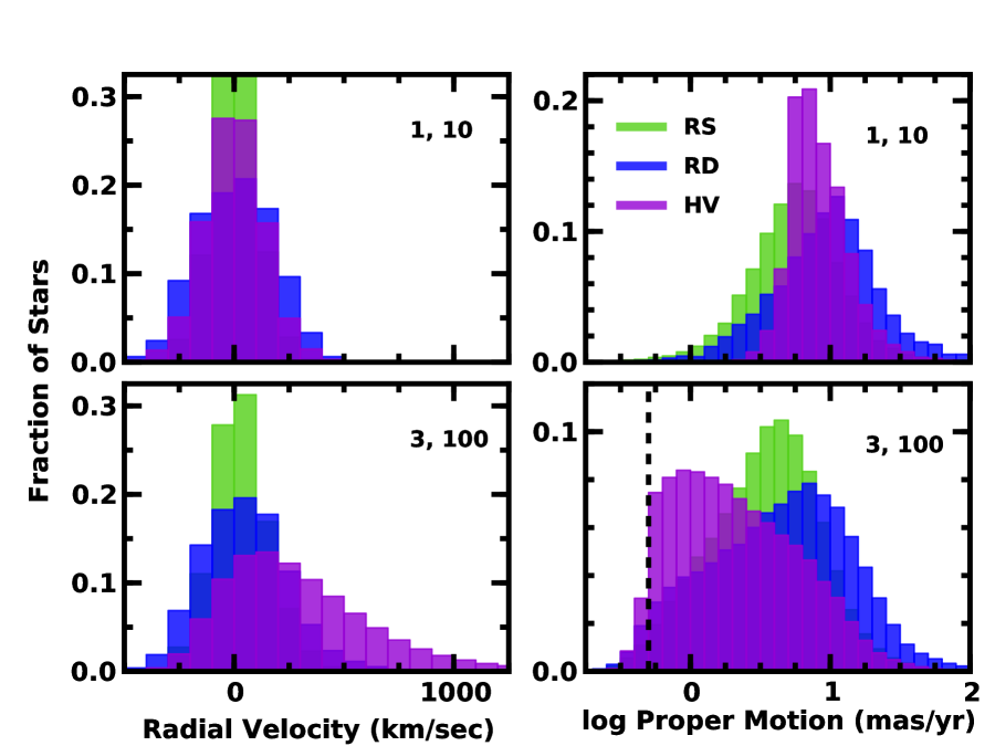
Figure 24: Predicted histograms of radial velocity (left panels) and proper motion (right panels) for distance-limited samples of HVSs (violet), supernova-induced runaways (green), and dynamically generated runaways (blue). The legend codifies the stellar mass (1 $M_{\odot}$ or 3 $M_{\odot}$) and the distance (10 kpc or 100 kpc). Dashed line in the lower right panel indicates the 3$\sigma$ GAIA detection limit for stars with $g\lesssim$ 20 (Lindegren, 2010).

To compare the distributions of proper motion and radial velocity in more detail, Fig. 24 shows histograms of radial velocity (left panels) and proper motion (right panels) for 1 $M_{\odot}$ (upper panels) and 3 $M_{\odot}$ (lower panels) ejected stars. The radial velocity histograms for 1 $M_{\odot}$ stars in the upper left panel are amazingly similar with clear peaks at roughly $-$50 km s^-1 and modest velocity dispersions. In this group, supernova-induced runaways have the smallest velocity dispersion, $\sim$ 103 km s^-1. HVSs have a somewhat smaller velocity dispersion, $\sim$ 138 km s^-1, than the dynamically generated runaways, $\sim$ 172 km s^-1 (Table 1).

Proper motion distributions for different types of 1 $M_{\odot}$ ejected stars are also very similar (Fig. 24, upper right panel). The HVSs have a sharp peak at 5–10 milliarcsec yr^-1; nearly all 1 $M_{\odot}$ HVSs have $\mu\approx$ 3–30 milliarcsec yr^-1. Runaways produced during a supernova have a broader distribution displaced to smaller $\mu$. The median $\mu$ is roughly 50% smaller; the dispersion is roughly 25% larger (Table 3). Dynamically generated runaways have median $\mu$ comparable to the HVSs and a 40% larger dispersion. Thus, the distribution of dynamically generated runaways extends to much larger $\mu$ than the HVSs.

The $v_{r}$ distributions for 3 $M_{\odot}$ stars are much easier to distinguish (Fig. 24, lower left panel). Supernova-induced runaways have a very narrow radial velocity distribution with a median near zero velocity and a dispersion of roughly 100 km s^-1 (see also Table 1). Dynamically generated runaways also have a median velocity near zero and a larger dispersion of 170 km s^-1. In contrast, 3 $M_{\odot}$ HVSs have a much larger median, $\sim$ 200 km s^-1, and dispersion, $\sim$ 300–350 km s^-1. More than 1% of the HVSs have radial velocities exceeding 1000 km s^-1, compared to 0% for both types of runaways.

The proper motion distributions of ejected 3 $M_{\odot}$ stars also show a clear separation (Fig. 24, lower right panel). Most high velocity HVSs lie at large distances and have small proper motions, producing a clear peak in the proper motion histogram at roughly 1 milliarcsec yr^-1. The distance limit establishes the sharp drop in the population at smaller $\mu$. A few nearby HVSs have maximum proper motions of 30–50 milliarcsec yr^-1.

Most 3 $M_{\odot}$ runaways have much larger proper motions than 3 $M_{\odot}$ HVSs. Stars ejected during a supernova have a fairly symmetric distribution of $\mu$, with a median at 3–5 milliarcsec yr^-1 and a dispersion of roughly 3–4 milliarcsec yr^-1. The dynamical ejections produce a broader peak with a larger median at roughly 8–9 milliarcsec yr^-1. Compared to the supernova-induced runaways, there are fewer dynamically generated runaways with $\mu\approx$ 3–5 milliarcsec yr^-1 and more with $\mu\approx$ 1–2 milliarcsec yr^-1.

8 OBSERVATIONAL TESTS

The distance-limited samples suggest several clear tests of the models based on existing samples of ejected stars. Among 3 $M_{\odot}$ stars, HVS models predict a much larger group of stars with large $v_{r}$ compared to either model for runaways. Because these stars lie at larger distances than runaways, HVSs should also have much smaller proper motions.

Among 1 $M_{\odot}$ stars, the models predict a large overlap in the observed $v_{r}$ and $\mu$. Despite this large overlap, it might be possible to isolate HVSs and dynamically generated runaways within a large sample of halo stars. The observed radial velocity dispersion of halo stars (100–110 km s^-1; e.g., Xue et al., 2008; Brown et al., 2010b; Gnedin et al., 2010; Piffl et al., 2014; Brown et al., 2014) is somewhat smaller than the predicted velocity dispersion – 140–170  km s^-1 – of HVSs and dynamically generated runaways. Large samples of stars might also provide a distinction between the narrow proper motion distribution predicted for HVSs from the broader distribution predicted for runaways.

To begin to investigate these possibilities, we consider several sets of ejected stars derived from the SDSS. For 1 $M_{\odot}$ stars, we examine candidates drawn from the G–K dwarfs in SEGUE (Yanny et al., 2009). The candidates have a broad range in brightness $g\approx$ 14–20. The large surface density of G–K dwarfs results in a sample of more than 28,000 stars with moderate resolution spectroscopy and high quality radial velocities and atmospheric parameters. From this ensemble, Palladino et al. (2014) use SDSS proper motion data to select 20 stars with $d\approx$ 1–6 kpc, $\mu\approx$ 10–100 milliarcsec yr^-1, and $v_{r}\approx$ $-200$ km s^-1 to $+130$ km s^-1. Most of these candidates are metal-poor, with $[{\rm Fe/H}]\approx$ $-1.27$ to $-0.06$ and modest enhancements of $\alpha$ nuclei relative to Fe.

To compare with models for 3 $M_{\odot}$ stars, we focus on the targeted search for HVSs from Brown et al. (2014). This set of $\sim$ 20 HVS candidates derives from a nearly complete spectroscopic survey of 1126 candidate B-type main sequence stars with $g\approx$ 17–20.25 selected from the SDSS (Brown et al., 2012b). Moderate resolution MMT spectra yield high quality radial velocities ($v_{r}\approx$ 250–800 km s^-1), atmospheric parameters (log $g\approx$ 3.75–4.6 and $T_{eff}\approx$ 10000–14000 K), and distances ($d\approx$ 40–100 kpc). For a few candidates, high resolution spectra confirm their main sequence nature and yield stronger constraints on the atmospheric parameters (López-Morales & Bonanos, 2008; Przybilla et al., 2008; Brown et al., 2012a, 2013).

To compare simulations with a sample of likely runaway stars, we select 16 runaway main sequence stars with high Galactic latitude and masses of 2.5–4.0 $M_{\odot}$ (Silva & Napiwotzki, 2011). Although derived from several surveys, this set of stars has reliable distances, radial velocities, proper motions, and atmospheric parameters. With $|v_{r}|\lesssim$ 250 km s^-1 and $d\lesssim$ 5 kpc, these runaways are closer and have much smaller space velocities than the HVS candidates. The accurate proper motions allow us to test whether the lack of proper motion information for the HVS candidates limits our ability to compare their radial velocity distributuon with our simulations.

To test the simulations in more detail, we examine a handful of miscellaneous high velocity main sequence stars identified in other surveys. In order of increasing mass, these stars are: SDSS J013655.91+242546.0, a 2.5 $M_{\odot}$ A-type sequence star with $d\approx$ 11 kpc and $v_{r}\approx$ 325 km s^-1 (Tillich et al., 2009); HIP 60350, a 5 $M_{\odot}$ B-type main sequence star with $d\approx$ 3 kpc and $v_{r}\approx$ 260 km s^-1 (Irrgang et al., 2010); HE0437-5439, a 9 $M_{\odot}$ B-type star close to the LMC with $d\approx$ 61 kpc and $v_{r}\approx$ 725 km s^-1 (Edelmann et al., 2005); HD 271791, an 11 $M_{\odot}$ B-type main sequence star with $d\approx$ 21 kpc and $v_{r}\approx$ 440 km s^-1 (Heber et al., 2008); and J091206.52+091621.8, another 11 $M_{\odot}$ B-type main sequence star with $d\approx$ 13 kpc and $v_{r}\approx$ 620 km s^-1 (Zheng et al., 2014). Selected in a variety of ways, this group of stars has reliable distances, space motions, and atmospheric properties. As with the runaways, the additional proper motion information yields a good test of our calculations.

Finally, we consider how well proper motion and radial velocity data isolate HVSs and runaways from samples of indigenous halo stars. For this study, we include data from recent surveys of halo stars towards the north Galactic pole (Kinman et al., 2007) and the Galactic anti-center (Kinman et al., 2012). Selected from several surveys, the RR Lyr stars have measured pulsation periods and metallicities; the blue horizontal branch (BHB) stars have no metallicity data. Both groups have proper motion and radial velocity measurements with typical uncertainties of a few milliarcsec yr^-1 and 10 km s^-1. With $\sim$ 100–125 confirmed halo stars in each sample, these data enable a first comparison between observations of halo stars and our calculations.

8.1 Surveys of solar-type stars

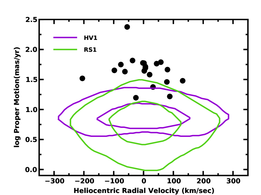
Figure 25: Comparison of observations for 1 $M_{\odot}$ candidates HVSs from Palladino et al. (2014) (filled circles) with predicted density contours in the $v_{r}$–$\mu$ plane for a distance-limited ($d$ = 10 kpc) sample of 1 $M_{\odot}$ HVSs (‘HV1’; violet curves) and 1 $M_{\odot}$ runaways (‘RS1’; green curves). For each model, the inner (outer) contours include 50% (90%) of stars in the the distance-limited samples. Aside from a few stars with $\mu\lesssim$ 30 milliarcsec yr^-1, the data fall well above predictions for either model.

Fig. 25 compares the HVS candidates from Palladino et al. (2014) with predictions from the HVS and supernova-induced runaway models. Solid lines show contours of constant stellar density which contain 50% (inner) and 90% (outer) of the stars in the complete samples of simulated stars. Contours for dynamically generated runaways are nearly identical to those for the supernova-induced runaways. Filled circles indicate the measured ($d,v_{r}$) for the HVS candidates.

Based on this comparison, the HVS model and both runaway models are wildly inconsistent with the observations. Although the observed radial velocities fall within the bounds predicted for all three models, the observed proper motions lie well above model predictions. None of the survey stars fall within the 50% contours of any model; only 3 fall within the 90% contours. Using the 95% contours (not shown on the Fig.), the runaway models fare a little better than the HVS model, with 5 (instead of 3) stars lying within the contours. Despite this marginally better success, all models are excluded at better than 3$\sigma$ confidence.

There are two possible origins of the mismatch between the models and the observations in Fig. 25. Reducing the proper motions by a factor of 5 would place the data within the 50% contours of all models. Although Palladino et al. (2014) derive high reliabilities for their proper motion measurements, the ratio of the transverse to radial velocity for this sample is much larger than expected for a random selection of high velocity stars. Thus, there is a reasonable probability that at least some of the large proper motions are spurious (Palladino et al., 2014). Testing this hypothesis with another epoch of imaging data from the ground or with GAIA is straightforward.

The only alternative to explain the large proper motions of these stars is to develop another model which produces high velocity stars. Modifying the existing HVS or runaway models is unlikely to produce a better match: the geometry of ejections from the GC or the Galactic disk simply precludes a large population of nearby 1 $M_{\odot}$ stars with modest radial velocity and very large proper motions. Supernova-induced runaways from binaries in the halo might allow a better match; however, supernova rates for halo binaries are probably much smaller than those in the disk. The Abadi et al. (2009) proposal of ejections from disrupted dwarf galaxies requires a somewhat massive Milky Way, $\sim$ 1.5–2 $\times 10^{12}$ $M_{\odot}$, but seems otherwise plausible. Numerical simulations of the velocity distribution of stars from disrupted dwarfs are required to test this interesting idea in more detail but are beyond the scope of this paper.

8.2 Surveys of B-type stars

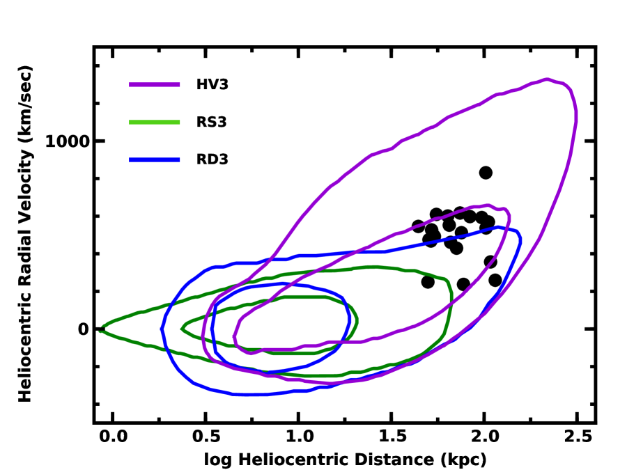
Figure 26: Comparison of observations for 3 $M_{\odot}$ candidates HVSs from Brown et al. (2014) (filled circles) with predicted density contours in the $d$–$v_{r}$ plane for a distance-limited ($d$ = 100 kpc) sample of 3 $M_{\odot}$ HVSs (‘HV3’; violet curves), 3 $M_{\odot}$ supernova-induced runaways (‘RS3’; green curves), and 3 $M_{\odot}$ dynamically generated runaways (‘RD3’; blue curves). For each model, the inner (outer) contours include 50% (90%) of stars in the the distance-limited samples. Although a few observations fall within the 90% contour for the dynamically generated runaway model, most (all) of the data fall within the 50% (90%) contours for the HVS model.

Fig. 26 compares the HVS candidates from Brown et al. (2014) with predictions from the HVS and runaway models. As in Fig. 25, solid lines show contours of stellar density which contain 50% (inner) and 90% (outer) of the stars in each simulation. Filled circles indicate the measured ($d,v_{r}$) for the HVS candidates. Unlike the 1 $M_{\odot}$ targets, these candidates lie close to or within the 90% contours for all three models.

This comparison strongly favors the HVS model for the origin of these high velocity stars. Only one (four) of the candidates lies within the 90% contour for the supernova-induced (dynamically generated) runaway model. Nearly all lie beyond the 95% contours (not shown on the Fig.). In contrast, more than half of the candidates lie within the 50% contour for the HVS model; all lie within the 90% contour. Taking the results at face value, this comparison rules out the runaway models at better than 3$\sigma$ confidence.

To test the models in another way, we attempt to match the observed $d$ and $v_{r}$ of the candidates from the complete ensemble of stars in the HVS and runaway models. For each HVS candidate with Galactic coordinates ($l,b$), we select all model stars within a 20^o $\times$ 20^o window centered on the measured coordinates. Among this group, we count the number of model stars with distances and radial velocities within 10% of the measurements and tabulate the number of ‘matches’ $N_{i}$ for each candidate.

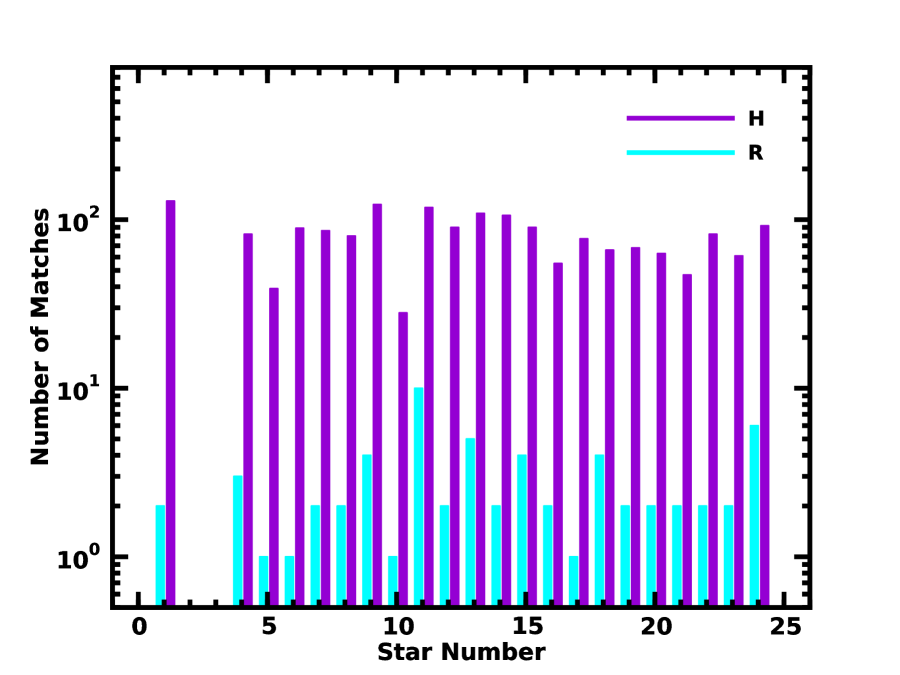
Figure 27: Distribution of matches between the 3 $M_{\odot}$ HVS (‘H’; violet) and runaway (‘R’; cyan) models and observations of HVSs candidates from Brown et al. (2014). For most known HVSs, the HVS model provides a better match to the data than the runaway model.

Fig. 27 summarizes the results of this matching exercise. For each survey star, the bars show $N_{i}$ for the HVS (violet) and dynamically generated runaway (cyan) models. With only one match among all HVS candidates, the supernova-induced runaway model fails the exercise. The HVS and dynamical runaway models fare much better, with $N_{i}\approx$ 30–100 for the HVS model and $N_{i}\approx$ 1–10 for the runaway model.

Based on this approach, we conclude with strong confidence that the candidate HVSs from the Brown et al. (2014) survey are much more likely to be HVSs ejected from the GC than runaway stars ejected from the Galactic disk. For every survey star, the HVS model yields a larger $N_{i}$ with $N_{i}({\rm HVS})\approx$ 10–100 $N_{i}({\rm runaway})$. Factor of two changes in the size of the windows for the distance, galactic coordinates, and radial velocity in the matching algorithm yield indistinguishable results. Among all HVS candidates, the supernova-induced runaway model yields 0–1 matches. Analyzing each candidate separately, an ensemble of HVSs ejected from the GC always produces a factor of 10–100 more matches than an ensemble of runaways generated from dynamical interactions.

Modest changes to the probability distribution for the ejection velocity of runaways cannot change this conclusion. Matching the observed radial velocities of the 3 $M_{\odot}$ HVS candidates requires much larger maximum ejection velocities (e.g., 800 km s^-1 instead of our adopted 400 km s^-1) for supernova-induced ejections or a much shallower power-law distribution of ejection velocities (e.g., $p_{D}(v_{ej})\propto v_{ej}^{-n}$, with $n\lesssim$ 2 instead of our adopted 8/3) for dynamically generated runaways. Although doubling the maximum velocity from a supernova ejection is possible in rare circumstances (e.g., Portegies Zwart, 2000), observations suggest a maximum ejection velocity of 400–450 km s^-1, close to our adopted value (e.g., Silva & Napiwotzki, 2011). Observations also appear to preclude placing a larger fraction of runaways at the highest velocities (Silva & Napiwotzki, 2011).

8.3 Runaway B-type Stars

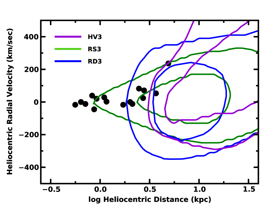
Figure 28: Comparison of observations (filled circles) for 3 $M_{\odot}$ runaway stars from Silva & Napiwotzki (2011) with predicted density contours in the $d$–$v_{r}$ plane for a distance-limited ($d$ = 100 kpc) sample of 3 $M_{\odot}$ HVSs (‘HV3’; violet curves), 3 $M_{\odot}$ supernova-induced runaways (‘RS3’; green curves), and 3 $M_{\odot}$ dynamically generated runaways (‘RD3’; blue curves). For each model, the inner (outer) contours include 50% (90%) of stars in the the distance-limited samples. Only two observations lie within the 90% contours for the HVS model. Although roughly half of the sample falls within the 90% contour for dynamically generated runaways, nearly all of the data fall within the 50%–90% contours for supernova-induced runaways.

Fig. 28 compares the runaways from Silva & Napiwotzki (2011) with predictions from the HVS and runaway models. As in Fig. 25, solid lines show contours of stellar density which contain 50% (inner) and 90% (outer) of the stars in each simulation. Filled circles indicate the measured ($d,v_{r}$) for the runaway candidates; these stars lie close to or within the 90% contours for all three models.

This comparison strongly favors the runaway model. Only two candidates lie within the 90% contour for the HVSs model; none lie within the 50% contour. Many of the candidates are close to or within contours from dynamically generated runaways with a minimum ejection velocity of 50 km s^-1. More than half of the candidates fall within the 90% contours of the supernova-induced runaway model. Contours generated from a set of dynamically generated runaways with a minimum ejection velocity of 20 km s^-1 show a similarly good agreement with the observations.

Our matching algorithm also favors the runaway model for these stars. Only one star – EC 09452-1403 with $v_{r}$ = 236 km s^-1 – yields any matches (three) to the HVS model. The supernova-induced runaway model typically yields 10–100 matches for each target.

To add a little more realism to the matching algorithm, we add the measured proper motions. Requiring the proper motion in $l$ and $b$ to match within $\pm$10% eliminates all matches for the HVS model to data for EC 09452-1403. Although including proper motion data also reduces the number of matches for the supernova-induced runaway model, the typical number of matches is still 3–20 per star.

These tests demonstrate our ability to explain observations of bona-fide runaways from a set of numerical simulations and to discriminate between HVSs and runaways. The positions of these stars in the $d-v_{r}$ diagram and the number of matches in $(d,\mu,v_{r})$ space clearly favor an identification as runaways rather than HVSs.

8.4 Miscellaneous High Velocity Stars

We now consider five miscellaneous high velocity stars identified as possible HVSs or ‘hyper-runaways.’ Here, we focus on two basic predictions from ejected star models: (i) HVSs should have radial orbits from the GC and (ii) runaways should have a significant non-radial component of motion consistent with ejection from the disk.

From the observed $l$, $b$, and $v_{r}$, we derive the radial velocity in the GC frame and the predicted proper motion for a purely radial orbit (e.g., eq. [5] and eqs. [12–14]). For nearby HVS candidates, the tangential component of the velocity dominates the space motion; for more distant HVSs, the radial component dominates. Among runaways, the tangential component of the motion is smaller than HVS for nearby stars and larger than HVS for more distant stars. If a nearby (distant) candidate is a runaway, we expect the analytic proper motion to exceed (fall below) the observed proper motion. In addition to yielding a reasonably simple way to distinguish between HVSs and runaways, this approach avoids cpu-intensive calculations for stars with masses of 2–11 $M_{\odot}$ which are not included in our suite of simulations.

To test this approach, we derive predicted proper motions for HVS candidates from Brown et al. (2014). Our analysis yields predictions of 0.3–1.2 milliarcsec yr^-1. For each HVS candidate, we then compare this analytic proper motion with the average proper motion from the simulated stars selected with the matching algorithm outlined in §8.3. The typical difference between the analytic and numerical results is small, $\sim$ 0.1–0.2 milliarcsec yr^-1, with a dispersion of 0.5 milliarcsec yr^-1. Thus, the analytic approach works reasonably well.

This analysis strongly favors runaway models for SDSS J013655.91+242546.0, HIP 60350, and HD 271791. For SDSS J013655.91+242546.0 and HD 271791, the observed magnitude of the proper motion is much larger than predicted from the simple HVS model. Coupled with the observed $v_{r}$, proper motions in $l$ and $b$ strongly favor ejection from the disk instead of the GC (see also Heber et al., 2008; Tillich et al., 2009). For HIP 60350, the HVS model predicts much larger proper motion than observed. Proper motions in $l$ and $b$ also favor a disk ejection (Irrgang et al., 2010).

For HE0437-5439 and J091206.52+091621.8, the small proper motions favor HVS models. HE0437-5439 has a distance and radial velocity similar to HVS-1 (Brown et al., 2005; Edelmann et al., 2005). HST proper motion data suggest origin in the GC (Brown et al., 2010a); ejection from the LMC is also possible (Edelmann et al., 2005; Brown et al., 2010a). For J091206.52+091621.8, the observed proper motion is comparable to or less than the predicted proper motion of roughly 3 milliarcsec yr^-1 (Zheng et al., 2014). However, the relatively large errors in the proper motion prevent isolating the ejection solely from the GC (Zheng et al., 2014).

8.5 Surveys of Halo Stars

To consider whether observations can distinguish HVSs and runaways from halo stars, we examine kinematic measurements from Kinman et al. (2007, 2012). Fig. 29 compares data for blue horizontal branch stars (‘BHB’; cyan points) and RR Lyr stars (‘RR’; orange points) with model contours for distance-limited samples of 3 $M_{\odot}$ HVSs (‘HV3’; violet curves) and runaways (‘RS3’; green curves). The contours enclose 50% (inner) and 95% (outer) of the stars in each simulation. To provide an approximate match to the Galactic coordinates for halo stars in the upper (lower) panel, we select HVSs and runaways with $b\geq$ 75^o ($l=$ 160^o to $l$ = 200^o and $b$ = 25^o to 50^o).

This comparison confirms our previous conclusion that radial velocity measurements directly discriminate between HVSs and indigenous halo stars (e.g., Brown et al., 2006; Bromley et al., 2006; Brown et al., 2007; Kenyon et al., 2008; Brown et al., 2009; Bromley et al., 2009; Brown et al., 2014). For $v_{r}\approx$ $-$200 km s^-1 to $+$300 km s^-1, the distributions of halo stars and HVSs overlap. Beyond $v_{r}\approx$ 300 km s^-1, however, HVSs dominate. This separation has a simple origin: HVSs and halo stars with $v_{r}\lesssim$ 300 km s^-1 are bound to the galaxy. HVSs with larger $v_{r}$ are unbound.

Although the radial velocity distributions for halo stars and runaways overlap in the direction of the north Galactic pole (NGP), the highest velocity runaways are easily distinguished from halo stars towards the Galactic anti-center. At the NGP, nearly all runaways are bound to the Galaxy. Thus, they have radial velocities similar to indigenous halo stars. Towards the anti-center, the velocity from Galactic rotation enables a significant population of unbound runaways on outbound trajectories. Bound halo stars never reach the large $v_{r}$ of these unbound runaways.

Proper motion data alone do not easily discriminate HVSs and runaways from indigenous halo stars. The maximum proper motion of halo stars in Kinman et al. (2007, 2012), $\sim$ 30–50 milliarcsec yr^-1, exceeds the proper motions of 99% ($\sim$ 100%) of HVSs and runaways towards the NGP (anti-center). Towards the anti-center, the number of high proper motion outliers, $\mu\gtrsim$ 100 milliarcsec yr^-1, is nearly zero. Towards the NGP, however, 0.1–1% of HVSs and runaways have proper motions larger than 100 milliarcsec yr^-1. Thus, occasional HVSs and runaways can be identified as proper motion outliers (e.g., Heber et al., 2008; Tillich et al., 2009; Irrgang et al., 2010).

For large samples of halo stars, accurate distances might provide a way to isolate runaways from indigenous stars (Fig. 12). Because runaways share the rotation of stars in the disk, they should exhibit a double-peaked distribution of proper motion. With little or no rotation (e.g., Bond et al., 2010), indigenous halo stars should have a single-peaked distribution. Although synthesizing the expected distribution for indigenous halo stars is beyond our scope, isolating the runaways probably requires a significant population of ejected stars within the halo.

8.6 Ejection Rates

To complete our comparisons between the models and available data, we now estimate the relative production rates for HVSs and runaways. Accurate rate estimates allow us to predict the relative space density of ejected stars as a function of distance and Galactic latitude (e.g., Brown et al., 2009; Bromley et al., 2009). Because the matching algorithm and the contour maps draw from equal numbers of simulated HVSs and runaways, production rates allow us to normalize the number of matches to the expected space density.

Predictions for HVSs depend on the rate binaries encounter the black hole at the GC (e.g., Yu & Tremaine, 2003). The time variation of the population of binaries within the ‘loss cone’ – the ensemble of orbits which pass within the black hole’s tidal radius – is an important issue in these derivations. Binary encounters with the black hole empty the loss cone; encounters between binaries and molecular clouds or other field stars fill the loss cone (e.g., Yu & Tremaine, 2003; Perets & Gualandris, 2010; Zhang et al., 2013; Vasiliev & Merritt, 2013; Madigan et al., 2014). Rates with a ‘full’ loss cone are larger than those with an ‘empty’ loss cone; typical estimates are $10^{-5}-10^{-3}$ yr^-1 for binaries of all types (e.g., Yu & Tremaine, 2003; Bromley et al., 2012; Zhang et al., 2013). For reasonable initial mass functions, limiting the binary population to 2.5–3.5 $M_{\odot}$ B-type stars (0.8–1.2 $M_{\odot}$ G-type stars) implies rates 40 times (10 times) smaller, 2.5–250 $\times 10^{-7}$ yr^-1 for B-type stars and 1–100 $\times 10^{-6}$ yr^-1 for G-type stars.

To infer empirical HVS rates, we focus on the S stars at the GC (Eckart & Genzel, 1997; Ghez et al., 1998) and HVSs in the Galactic halo (Brown et al., 2014). The S stars are luminous B-type stars orbiting the GC which are the plausible captured partners of HVSs ejected into the outer Galaxy (Gould & Quillen, 2003; O’Leary & Loeb, 2008; Perets, 2009; Madigan et al., 2014). The population of S stars implies a capture rate of roughly $2\times 10^{-7}$ yr^-1 for stars with masses exceeding 5 $M_{\odot}$ (see also Bromley et al., 2012). Using their complete spectroscopic sample of B-type stars in the outer halo, Brown et al. (2014) estimate a production rate of $1.5\times 10^{-6}$ yr^-1 for unbound HVSs with masses of 2.5–4 $M_{\odot}$. For an ensemble of stars selected from a Salpeter IMF, these rates agree with theoretical predictions and with each other to within a factor of two.

Predictions rates for runaways from supernovae depend on the local star formation rate, the mass range adopted for B-type stars, the fraction of stars in binaries, and the fraction of binaries with mass ratios and orbital periods capable of ejecting a star with a velocity exceeding 10–20 km s^-1 (e.g., Brown et al., 2009; Bromley et al., 2009). For a star formation rate of 0.5 $M_{\odot}~{}{\rm yr}^{-1}$ (Lada & Lada, 2003) and for the observed properties of binaries composed of B-type stars with masses of 2.5–4 $M_{\odot}$ (Kobulnicky & Fryer, 2007), supernovae produce runaways with minimum ejection velocities of 10 km s^-1 at a rate of roughly $3\times 10^{-6}$ yr^-1 (see also Brown et al., 2009; Bromley et al., 2009).

Predicting ejection rates for the dynamical runaway mechanism is more challenging. From numerical simulations of dense clusters, Perets & Subr (2012) estimate an ejection rate for hyper-runaway B-type stars with $v_{esc}\gtrsim$ 450 km s^-1 of $1-2\times 10^{-8}$ yr^-1. For a power-law probability of the ejection velocity (eq. [26]), the total ejection rate for B-type runaway stars with $v_{esc}\gtrsim$ 10 km s^-1, is roughly $1-2\times 10^{-5}$ yr^-1. This rate suggests that dynamically generated runaways are somewhat more common than supernova-induced runaways.

Empirical rates for runaways generally agree with these estimates. To derive these rates, we estimate the formation rate of 2.5–3.5 $M_{\odot}$ stars from the observed star formation rates and a Salpeter initial mass function. For the Lada & Lada (2003) star formation rate of 0.5 $M_{\odot}~{}{\rm yr}^{-1}$, one star with a mass of 2.5–3.5 $M_{\odot}$ is born every 300–350 years. To infer the fraction of runaway stars in this group, we rely on the observed frequencies of less than 1% for A-type stars (Stetson, 1981; Bromley et al., 2009), 5% for B-type stars (Gies & Bolton, 1986), and more than 20% for O-type stars (Tetzlaff et al., 2011). Adopting a 1–2% runaway frequency among 2.5–3.5 $M_{\odot}$ stars yields a production rate of $3-6\times 10^{-5}$ yr^-1. This rate is nearly identical to our purely theoretical rate estimate.

Altogether, these estimates suggest our matching algorithm selects stars from ensembles with similar formation rates. If we assume that bound HVSs have a comparable frequency to unbound HVSs in the Brown et al. (2014) sample, the combined HVS production rate of $3\times 10^{-6}$ yr^-1 is identical to the production rate of supernova-induced runaways. For the dynamically generated runaways, we correct the complete ensemble for the fraction of runaways with $v_{ej}\gtrsim$ 50 km s^-1. This correction yields an expected rate of $3-6\times 10^{-6}$ yr^-1, very close to the rates for HVSs and supernova-induced runaways.

Although these estimates yield roughly similar production rates for HVSs and both types of runaways, we expect unbound runaways to be much less frequent than unbound HVSs. More than 25% of HVSs ejected from the GC to distances $\geq$ 10 kpc are unbound (§5). In contrast, $\leq$ 1% of runaways have ejection velocities larger than the local escape velocity. Thus, unbound HVSs should greatly outnumber unbound runaways in the halo.

Overall, observations confirm the expectation that the number of unbound runaways is smaller then the number of unbound HVSs (see also Brown et al., 2009; Bromley et al., 2009; Perets & Subr, 2012). For every unbound runaway, theory predicts 10–30 HVSs. Among known unbound stars, the vast majority are HVSs (§8.3; see also Brown et al., 2009).

8.7 Summary

Observations of HVS candidates and known runaways yield good tests of the numerical simulations. The comparisons in the preceding subsections lead to several clear conclusions.

• Runaway models provide an excellent match to observations of known runaway stars with modest radial velocities, $v_{r}\lesssim$ 250 km s^-1 (Silva & Napiwotzki, 2011).

• The HVS models match observations of HVS candidates from Brown et al. (2014).

• HVS and runaway star models fail to match observations of HVS candidates from SEGUE (Palladino et al., 2014). If the proper motions are correct, some other model for ejected stars is required to match the observations.

• Among a few miscellaneous high velocity stars, at least three are runaways (Heber et al., 2008; Tillich et al., 2009; Irrgang et al., 2010). Two others are more likely HVSs (Edelmann et al., 2005; Brown et al., 2010a; Zheng et al., 2014).

• Cleanly isolating unbound ejected stars from indigenous halo stars requires radial velocities. If the halo contains a large population of runaways ejected from the disk, these stars can be identified as high proper motion outliers or by their rotational motion about the GC.

• Observed and theoretical formation rates for HVSs and runaways suggest that most unbound stars in the halo are HVSs.

9 DISCUSSION AND SUMMARY

We have explored analytic treatments and have developed numerical calculations of HVSs and runaway stars moving through the Galaxy. The simulations use a realistic Galactic potential which matches observations in the GC, the bulge, the disk, and the halo. Algorithms for the velocities of ejected stars are based on detailed analytic and numerical calculations of (i) binaries interacting with the black hole in the GC, (ii) binaries where one component undergoes a supernova explosion, and (iii) single and multiple stars interacting in a massive star cluster. Realistic main sequence lifetimes allow snapshots of the positions and space motions for ejected stars as a function of time.

The following theoretical results serve as a guide for interpreting data from large-scale surveys with GAIA and ground-based telescopes.

• Ejected stars have a broad range in radial velocity ($v_{r}\approx$ 0–1000 km s^-1) and proper motion ($\mu\approx$ 0.01–100 milliarcsec yr^-1).

• At all distances, HVSs have larger space velocities than runaways. For $d\approx$ 50–150 kpc, unbound HVSs dominate the population. Nearby ($d\lesssim$ 10 kpc), unbound stars are rare; bound HVSs and runaways are common.

• For nearby stars with $d\lesssim$ 10 kpc, proper motions cannot isolate high velocity ejected stars from horizontal branch stars in the halo.

• At larger distances, radial velocities excel at distinguishing ejected stars from indigenous halo stars.

• For runaway stars ejected into the halo at $d\approx$ 20–50 kpc, a double-peaked proper motion distribution results from orbital motion around the GC. This distribution cleanly separates runaways from either HVSs or halo stars on radial orbits.

• Concentrations of high proper motion stars near the GC are a unique signature of HVSs ejected from the GC or runaways ejected from the inner galaxy.

These general conclusions are fairly independent of the modeling approach. The main trends for bound and unbound stars depend on the point of origin (GC for HVSs or disk for runaways) and the total mass of the Galaxy within roughly 10 kpc (e.g., Kenyon et al., 2008). Thus, modest changes to the mass of the Galaxy, the mass in the bulge, disk, or halo, or to the velocity distributions of ejected stars cannot modify our main conclusions. Adopting a triaxial potential for the bulge or a more realistic disk-like potential for the GC can modify the median velocities, the velocity dispersions, and the relative densities of HVSs with Galactic latitude and longitude (e.g., Gnedin et al., 2005; Yu & Madau, 2007; Lu et al., 2010; Zhang et al., 2010; Rossi et al., 2013). However, tests with realistic anisotropic potentials show that the general trends do not depend on the form of the Galactic potential. Similarly, modest changes in the adopted velocity distributions of ejected stars yield modest differences in the shape of the predicted distributions of $v_{r}$ and $\mu$ with distance without changing the nature of systematic variations with distance and Galactic coordinates.

Comparisons between these predictions and existing observations of ejected stars are encouraging. Several large surveys of HVSs and runaways demonstrate several unambiguous conclusions.

• Simulations of supernova-induced and dynamically generated runaways match observations of known runaway stars with modest radial velocities, $v_{r}\lesssim$ 250 km s^-1 (Silva & Napiwotzki, 2011). HVS models fail to match these data.

• HVS models explain observations of HVS candidates from Brown et al. (2014). Runaway star models cannot explain the data.

• HVS and runaway star models fail to account for observations of HVS candidates from SEGUE (Palladino et al., 2014). If the proper motions of the SEGUE candidates are correct, another model for ejected stars is required to match the observations.

• Among a few miscellaneous high velocity stars, at least three are runaways (Heber et al., 2008; Tillich et al., 2009; Irrgang et al., 2010). Two others are more likely HVSs (Brown et al., 2010a; Zheng et al., 2014).

• Observed and theoretical formation rates for HVSs and runaways suggest that most unbound stars in the halo are HVSs.

GAIA data will provide clear tests of the theoretical predictions and observational comparisons outlined above. For solar-type stars with $g\lesssim$ 20, GAIA data will yield robust samples of high velocity stars with $\mu\gtrsim$ 0.5 milliarcsec yr^-1 and $d\lesssim$ 10 kpc. Within this group, quantifying the (probably very low) fraction of unbound stars can place useful limits on the velocity distributions of ejected stars. More likely, identifying outliers in the distributions of proper motion and radial velocity will yield a population of bound HVSs and runaways. Aside from the properties of ejected stars, comparisons with theoretical models can yield information on the potential of the bulge and inner disk.

Accurate GAIA proper motions ($\delta\mu\lesssim$ 0.16 milliarcsec yr^-1) for stars with $g\lesssim$ 20 (Lindegren, 2010; Lindegren et al., 2012), high quality radial velocities from large ground-based telescopes (e.g., Brown et al., 2014), and good spectroscopic parallaxes will probe the properties of unbound B-type stars out to $d\approx$ 100 kpc. These data will yield improved constraints on (i) the production rates for HVSs and runaways and (ii) the relative populations of bound and unbound stars.

Although GAIA can identify stars with masses of roughly 10 $M_{\odot}$ to much larger distances, the shorter main sequence lifetimes of these stars preclude large populations beyond 20–30 kpc (see also Bromley et al., 2006, 2009). If ejections of very massive HVSs or runaways are more frequent than those of 3 $M_{\odot}$ stars, GAIA could discover a few massive, very high velocity ejected stars beyond 100 kpc.

As dynamical models for ejected stars improve, GAIA observations of the complete sample of 1–10 $M_{\odot}$ HVSs and runaways will enable new measurements of anisotropies in the shape of the Galactic potential (Gnedin et al., 2005; Yu & Madau, 2007). HVSs and runaways near the GC constrain the shape of the bulge. More distant stars probe the shape of the halo. Together, HVSs and runaways in the bulge and halo may yield new insights into the distribution of dark matter throughout the Galaxy.

We acknowledge generous allotments of computer time on the NASA ‘discover’ cluster. Clear and respectful comments from an anonymous referee improved our presentation.

Table 1: Radial Velocity Statistics for Runaway and Hypervelocity Stars

Model	d (kpc)	$f_{d}$ (%)	$v_{med}$ (km s-1)	$v_{q1}$ (km s-1)	$v_{q3}$ (km s-1)	$v_{avg}$ (km s-1)	$\sigma_{r}$ (km s-1)
HV1	0–10	2.96	$-$0.3	$-$89.3	89.7	0.9	138.3
HV1	10–20	2.54	5.1	$-$113.6	126.0	9.2	188.7
HV1	20–40	1.73	15.9	$-$128.5	158.7	25.2	233.9
HV1	40–80	1.12	39.5	$-$110.4	197.5	67.9	275.3
HV1	80–160	0.86	90.8	$-$71.5	292.8	152.7	337.3
HV3	0–10	2.80	31.6	$-$70.7	146.6	55.8	190.4
HV3	10–20	3.10	167.3	2.8	362.5	208.5	297.0
HV3	20–40	3.74	268.8	83.2	498.3	321.5	339.7
HV3	40–80	3.77	395.1	209.1	635.9	457.3	355.6
HV3	80–160	2.77	605.9	414.5	855.6	672.1	367.9
RS1	0–10	2.28	1.9	$-$60.7	65.1	2.0	102.9
RS1	10–20	1.07	4.9	$-$88.1	95.8	3.2	132.9
RS1	20–40	0.48	2.4	$-$107.3	113.8	3.8	158.6
RS1	40–80	0.15	5.8	$-$114.7	128.6	8.5	169.1
RS1	80–160	0.03	1.1	$-$113.7	125.3	10.6	170.4
RS3	0–10	2.30	10.1	$-$51.4	75.6	12.9	103.6
RS3	10–20	1.11	27.7	$-$64.4	121.2	29.1	135.4
RS3	20–40	0.60	59.9	$-$51.1	172.1	61.5	159.0
RS3	40–80	0.28	106.7	$-$10.5	219.9	107.1	154.3
RS3	80–160	0.03	187.6	67.9	314.1	192.8	143.9
RD1	0–10	0.27	9.7	$-$120.0	130.8	6.1	171.7
RD1	10–20	0.11	$-$7.3	$-$126.6	124.2	$-$1.1	172.2
RD1	20–40	0.05	15.3	$-$115.9	141.4	12.7	185.5
RD1	40–80	0.02	12.0	$-$112.2	157.4	25.2	201.5
RD1	80–160	0.01	30.9	$-$118.5	151.8	25.9	194.5
RD3	0–10	0.26	4.5	$-$121.0	128.7	5.1	173.6
RD3	10–20	0.12	35.8	$-$90.1	162.3	41.5	181.7
RD3	20–40	0.06	96.2	$-$44.7	239.4	108.9	211.5
RD3	40–80	0.04	188.5	54.9	331.7	202.4	205.0
RD3	80–160	0.02	341.4	214.9	471.4	347.4	184.9
RT1	0–10	2.43	5.2	$-$170.7	176.6	3.6	216.7
RT1	0–20	4.72	4.4	$-$161.2	172.2	5.6	214.9
RT1	0–40	6.06	7.3	$-$141.4	157.1	8.2	206.9
RT1	0–80	5.29	9.2	$-$124.6	145.1	11.6	195.1
RT1	80–160	3.54	20.5	$-$105.0	150.7	25.5	186.4
RT3	0–10	2.67	86.1	$-$100.8	255.7	77.2	225.6
RT3	10–20	5.19	129.4	$-$49.1	286.3	118.7	220.6
RT3	20–40	7.96	167.2	6.0	323.0	165.4	214.3
RT3	40–80	10.46	204.9	80.3	338.2	213.4	184.6
RT3	80–160	6.64	301.3	194.4	418.9	308.5	156.1

Note. — $f_{d}$: fraction of stars; $v_{med}$: median velocity; $v_{q1},v_{q3}$: inter-quartile range; $v_{avg}$: average velocity; $\sigma_{r}$: standard deviation in radial velocity; HV1, HV3: 1 $M_{\odot}$, 3 $M_{\odot}$ HVS models; RS1, RS3: 1 $M_{\odot}$, 3 $M_{\odot}$ supernova-induced runaway models; RD1, RD3: 1 $M_{\odot}$, 3 $M_{\odot}$ dynamically generated runaway models; RT1, RT3: 1 $M_{\odot}$, 3 $M_{\odot}$ toy runaway models

Table 2: Tangential Velocity Statistics for Runaway and Hypervelocity Stars

Model	d (kpc)	$f_{d}$ (%)	$v_{med}$ (km s-1)	$v_{q1}$ (km s-1)	$v_{q3}$ (km s-1)	$v_{avg}$ (km s-1)	$\sigma_{t}$ (km s-1)
HV1	0–10	2.96	243.8	218.8	285.0	257.1	74.3
HV1	10–20	2.54	232.8	205.7	248.4	230.3	50.3
HV1	20–40	1.73	219.4	190.7	234.7	211.5	36.4
HV1	40–80	1.12	214.2	185.1	231.4	205.8	31.5
HV1	80–160	0.86	214.7	186.6	230.9	205.5	30.0
HV3	0–10	2.80	251.6	221.5	325.1	299.6	156.7
HV3	10–20	3.10	242.2	216.7	297.2	274.1	112.5
HV3	20–40	3.74	232.6	206.4	252.4	235.9	56.9
HV3	40–80	3.77	226.4	198.8	238.3	219.1	35.5
HV3	80–160	2.77	222.6	195.5	235.5	212.9	30.0
RS1	0–10	2.28	129.5	79.9	195.0	145.3	87.8
RS1	10–20	1.07	199.3	134.0	293.6	217.8	107.9
RS1	20–40	0.48	204.7	146.2	296.2	220.8	93.7
RS1	40–80	0.15	181.7	146.4	263.9	201.7	70.1
RS1	80–160	0.03	187.3	155.4	246.3	197.6	56.3
RS3	0–10	2.30	129.2	80.1	193.6	145.2	87.3
RS3	10–20	1.11	197.7	133.4	291.2	215.6	106.4
RS3	20–40	0.60	189.9	140.5	289.2	213.8	93.7
RS3	40–80	0.28	185.0	148.9	269.5	205.9	72.7
RS3	80–160	0.03	186.3	150.3	265.5	204.3	64.0
RD1	0–10	0.27	250.2	152.6	360.2	260.8	134.6
RD1	10–20	0.11	229.3	142.7	324.3	236.1	115.2
RD1	20–40	0.05	204.5	148.9	281.7	216.8	85.5
RD1	40–80	0.02	211.7	169.4	253.5	212.4	58.9
RD1	80–160	0.01	210.8	174.5	235.0	206.6	40.6
RD3	0–10	0.26	255.2	153.3	365.7	262.1	134.0
RD3	10–20	0.12	232.6	142.5	327.4	237.8	116.2
RD3	20–40	0.06	209.9	148.5	286.8	218.7	90.6
RD3	40–80	0.04	198.8	161.6	252.4	206.5	61.4
RD3	80–160	0.02	203.2	171.8	239.9	204.8	45.4
RT1	0–10	2.43	316.5	244.5	393.1	320.0	111.7
RT1	10–20	4.72	243.7	180.8	312.6	252.8	104.1
RT1	20–40	6.06	218.9	177.0	265.2	221.2	66.9
RT1	40–80	5.29	211.8	180.8	245.7	211.6	47.4
RT1	80–160	3.54	208.3	180.2	233.8	205.4	38.0
RT3	0–10	2.67	86.1	$-$100.8	255.7	77.2	225.6
RT3	10–20	5.19	129.4	$-$49.1	286.3	118.7	220.6
RT3	20–40	7.96	167.2	6.0	323.0	165.4	214.3
RT3	40–80	10.46	204.9	80.3	338.2	213.4	184.6
RT3	80–160	6.64	301.3	194.4	418.9	308.5	156.1

Note. — $f_{d}$: fraction of stars; $v_{med}$: median velocity; $v_{q1},v_{q3}$: inter-quartile range; $v_{avg}$: average velocity; $\sigma_{t}$: standard deviation in tangential velocity; HV1, HV3: 1 $M_{\odot}$, 3 $M_{\odot}$ HVS models; RS1, RS3: 1 $M_{\odot}$, 3 $M_{\odot}$ supernova-induced runaway models; RD1, RD3: 1 $M_{\odot}$, 3 $M_{\odot}$ dynamically generated runaway models; RT1, RT3: 1 $M_{\odot}$, 3 $M_{\odot}$ toy runaway models

Table 3: Proper Motion Statistics for Runaway and Hypervelocity Stars

Model	d (kpc)	$f_{d}$ (%)	log $\mu_{med}$	log $\mu_{q1}$	log $\mu_{q3}$	(${\rm log}~{}\mu)_{avg}$	$\sigma({\rm log}~{}\mu)$
HV1	0–10	2.96	0.89	0.77	1.04	0.92	0.22
HV1	10–20	2.54	0.54	0.44	0.63	0.54	0.14
HV1	20–40	1.73	0.20	0.12	0.29	0.20	0.12
HV1	40–80	1.12	$-$0.11	$-$0.19	$-$0.02	$-$0.11	0.11
HV1	80–160	0.86	$-$0.42	$-$0.50	$-$0.33	$-$0.42	0.11
HV3	0–10	2.80	0.94	0.80	1.11	0.98	0.25
HV3	10–20	3.10	0.56	0.46	0.67	0.58	0.18
HV3	20–40	3.74	0.23	0.14	0.32	0.23	0.14
HV3	40–80	3.77	$-$0.09	$-$0.17	0.00	$-$0.09	0.12
HV3	80–160	2.77	$-$0.39	$-$0.47	$-$0.31	$-$0.39	0.11
RS1	0–10	2.28	0.75	0.55	0.95	0.74	0.34
RS1	10–20	1.07	0.49	0.30	0.65	0.46	0.26
RS1	20–40	0.48	0.21	0.04	0.37	0.20	0.23
RS1	40–80	0.15	$-$0.12	$-$0.25	0.01	$-$0.12	0.17
RS1	80–160	0.03	$-$0.41	$-$0.52	$-$0.30	$-$0.41	0.15
RS3	0–10	2.30	0.75	0.55	0.95	0.74	0.34
RS3	10–20	1.11	0.48	0.30	0.64	0.46	0.26
RS3	20–40	0.60	0.17	0.01	0.34	0.17	0.23
RS3	40–80	0.28	$-$0.12	$-$0.24	0.02	$-$0.11	0.18
RS3	80–160	0.03	$-$0.36	$-$0.46	$-$0.22	$-$0.35	0.15
RD1	0–10	0.27	0.99	0.73	1.20	0.97	0.41
RD1	10–20	0.11	0.55	0.33	0.71	0.50	0.29
RD1	20–40	0.05	0.20	0.05	0.34	0.19	0.22
RD1	40–80	0.02	$-$0.10	$-$0.21	0.02	$-$0.10	0.16
RD1	80–160	0.01	$-$0.38	$-$0.51	$-$0.30	$-$0.41	0.14
RD3	0–10	1.04	0.98	0.74	1.19	0.96	0.39
RD3	10–20	0.45	0.55	0.33	0.71	0.50	0.29
RD3	20–40	0.24	0.19	0.03	0.34	0.18	0.23
RD3	40–80	0.17	$-$0.13	$-$0.24	$-$0.01	$-$0.12	0.16
RD3	80–160	0.09	$-$0.40	$-$0.49	$-$0.31	$-$0.40	0.13
RT1	0–10	2.43	0.99	0.83	1.15	0.99	0.28
RT1	10–20	4.72	0.53	0.39	0.67	0.52	0.23
RT1	20–40	6.06	0.20	0.09	0.31	0.19	0.17
RT1	40–80	5.29	$-$0.10	$-$0.20	$-$0.01	$-$0.11	0.14
RT1	80–160	3.54	$-$0.41	$-$0.50	$-$0.32	$-$0.41	0.12
RT3	0–10	2.67	0.99	0.83	1.16	0.99	0.29
RT3	10–20	5.19	0.53	0.38	0.68	0.52	0.24
RT3	20–40	7.96	0.20	0.07	0.32	0.19	0.19
RT3	40–80	10.46	$-$0.12	$-$0.22	$-$0.01	$-$0.12	0.15
RT3	80–160	6.64	$-$0.39	$-$0.48	$-$0.30	$-$0.40	0.13

Note. — $f_{d}$: fraction of stars; $\mu_{med}$: median proper motion; $\mu_{q1},\mu_{q3}$: inter-quartile range; $({\rm log}~{}\mu)_{avg}$: average log proper motion; $\sigma({\rm log}~{}\mu)$: standard deviation in log proper motion; all proper motions in units of milliarcsec yr^-1; HV1, HV3: 1 $M_{\odot}$, 3 $M_{\odot}$ HVS models; RS1, RS3: 1 $M_{\odot}$, 3 $M_{\odot}$ supernova-induced runaway models; RD1, RD3: 1 $M_{\odot}$, 3 $M_{\odot}$ dynamically generated runaway models; RT1, RT3: 1 $M_{\odot}$, 3 $M_{\odot}$ toy runaway models

Figure 4: As in Fig. 3 in the heliocentric galactic frame. In a frame centered on the Sun, stars inside the solar circle (cyan lines) have a maximum galactic longitude, $l_{max}$ (eq. [1]). The tangential velocity ($|v_{t}|$) reaches a maximum and a minimum at $l$ = 0. The radial velocity achieves extreme values at $\pm l_{max}$. Outside the solar circle (magenta lines), $v_{r}$ and $v_{t}$ follow simple sinusoids, with extreme values at $\pm\pi/2$ ($v_{r}$) and at 0 and $\pm\pi$ ($v_{t}$).

Figure 19: Histograms of proper motions for HVSs (top panels), runaways produced during a supernova (middle panels), and runaways from dynamical ejections (lower panels) with $|b|\geq$ 30 ^o. Left panels: histograms for 1 $M_{\odot}$ stars; right panels: histograms for 3 $M_{\odot}$ stars; dashed lines indicate the 3$\sigma$ GAIA detection limit for stars with $g\lesssim$ 20 (Lindegren, 2010). Among long-lived 1 $M_{\odot}$ stars, unbound stars at large distances ($d\gtrsim$ 100 kpc) have small proper motions $\mu\approx 10^{-2}-10^{-1}$ milliarcsec yr^-1. Unbound higher mass stars do not live long enough to reach $d\gtrsim$ 100 kpc; they have proper motions $\mu\approx$ 0.1–1 milliarcsec yr^-1. Bound stars of any mass have small distances, $d\lesssim$ 20–30 kpc, and modest proper motions, $\mu\approx$ 1–10 milliarcsec yr^-1.

Figure 29: Comparison of observations (filled circles) for RR Lyr (‘RR’; orange points) and BHB (‘BHB’; cyan points) stars from Kinman et al. (2007, 2012) with predicted density contours in the $v_{r}$–$\mu$ plane for a distance-limited ($d$ = 100 kpc) sample of 3 $M_{\odot}$ HVSs (‘HV3’; violet curves) and 3 $M_{\odot}$ supernova-induced runaways (‘RS3’; green curves). Typical errors are $\pm$1–2 milliarcsec yr^-1 for $\mu$ and $\pm$10 km s^-1 for $v_{r}$. Survey limits and measurement errors preclude stars with $\mu\lesssim$ 1–3 milliarcsec yr^-1 in each panel. For each model, the inner (outer) contours include 50% (95%) of stars in the the distance-limited samples. Upper panel: stars in the direction of the north Galactic pole (NGP). Lower panel: stars in the direction of the Galactic anti-center (AC). The halo star observations uniformly fill the upper half of the contours for runaway stars and the low velocity portion of the HVS model contours.

References

- Abadi et al. (2009) Abadi, M. G., Navarro, J. F., & Steinmetz, M. 2009, ApJ, 691, L63
- Abt (1983) Abt, H. A. 1983, ARA&A, 21, 343
- Binney & Tremaine (2008) Binney, J., & Tremaine, S. 2008, Galactic Dynamics: Second Edition (Princeton University Press)
- Blaauw (1961) Blaauw, A. 1961, Bull. Astron. Inst. Netherlands, 15, 265
- Bond et al. (2010) Bond, N. A., et al. 2010, ApJ, 716, 1
- Bovy & Rix (2013) Bovy, J., & Rix, H.-W. 2013, ApJ, 779, 115
- Bovy et al. (2012) Bovy, J., et al. 2012, ApJ, 759, 131
- Brand & Wouterloot (2007) Brand, J., & Wouterloot, J. G. A. 2007, A&A, 464, 909
- Bressan et al. (2012) Bressan, A., Marigo, P., Girardi, L., Salasnich, B., Dal Cero, C., Rubele, S., & Nanni, A. 2012, MNRAS, 427, 127
- Bromley & Kenyon (2006) Bromley, B. C., & Kenyon, S. J. 2006, AJ, 131, 2737
- Bromley et al. (2009) Bromley, B. C., Kenyon, S. J., Brown, W. R., & Geller, M. J. 2009, ApJ, 706, 925
- Bromley et al. (2006) Bromley, B. C., Kenyon, S. J., Geller, M. J., Barcikowski, E., Brown, W. R., & Kurtz, M. J. 2006, ApJ, 653, 1194
- Bromley et al. (2012) Bromley, B. C., Kenyon, S. J., Geller, M. J., & Brown, W. R. 2012, ApJ, 749, L42
- Brown et al. (2010a) Brown, W. R., Anderson, J., Gnedin, O. Y., Bond, H. E., Geller, M. J., Kenyon, S. J., & Livio, M. 2010a, ApJ, 719, L23
- Brown et al. (2012a) Brown, W. R., Cohen, J. G., Geller, M. J., & Kenyon, S. J. 2012a, ApJ, 754, L2
- Brown et al. (2013) —. 2013, ApJ, 775, 32
- Brown et al. (2009) Brown, W. R., Geller, M. J., & Kenyon, S. J. 2009, ApJ, 690, 1639
- Brown et al. (2012b) —. 2012b, ApJ, 751, 55
- Brown et al. (2014) —. 2014, ApJ, 787, 89
- Brown et al. (2010b) Brown, W. R., Geller, M. J., Kenyon, S. J., & Diaferio, A. 2010b, AJ, 139, 59
- Brown et al. (2005) Brown, W. R., Geller, M. J., Kenyon, S. J., & Kurtz, M. J. 2005, ApJ, 622, L33
- Brown et al. (2006) —. 2006, ApJ, 640, L35
- Brown et al. (2007) Brown, W. R., Geller, M. J., Kenyon, S. J., Kurtz, M. J., & Bromley, B. C. 2007, ApJ, 660, 311
- de Zeeuw et al. (1999) de Zeeuw, P. T., Hoogerwerf, R., de Bruijne, J. H. J., Brown, A. G. A., & Blaauw, A. 1999, AJ, 117, 354
- Dehnen et al. (2006) Dehnen, W., McLaughlin, D. E., & Sachania, J. 2006, MNRAS, 369, 1688
- Duquennoy & Mayor (1991) Duquennoy, A., & Mayor, M. 1991, A&A, 248, 485
- Eckart & Genzel (1997) Eckart, A., & Genzel, R. 1997, MNRAS, 284, 576
- Edelmann et al. (2005) Edelmann, H., Napiwotzki, R., Heber, U., Christlieb, N., & Reimers, D. 2005, ApJ, 634, L181
- Genzel et al. (2010) Genzel, R., Eisenhauer, F., & Gillessen, S. 2010, Reviews of Modern Physics, 82, 3121
- Ghez et al. (1998) Ghez, A. M., Klein, B. L., Morris, M., & Becklin, E. E. 1998, ApJ, 509, 678
- Gies & Bolton (1986) Gies, D. R., & Bolton, C. T. 1986, ApJS, 61, 419
- Ginsburg & Loeb (2007) Ginsburg, I., & Loeb, A. 2007, MNRAS, 376, 492
- Gnedin et al. (2010) Gnedin, O. Y., Brown, W. R., Geller, M. J., & Kenyon, S. J. 2010, ApJ, 720, L108
- Gnedin et al. (2005) Gnedin, O. Y., Gould, A., Miralda-Escudé, J., & Zentner, A. R. 2005, ApJ, 634, 344
- Gould & Quillen (2003) Gould, A., & Quillen, A. C. 2003, ApJ, 592, 935
- Heacox (1998) Heacox, W. D. 1998, AJ, 115, 325
- Heber et al. (2008) Heber, U., Edelmann, H., Napiwotzki, R., Altmann, M., & Scholz, R.-D. 2008, A&A, 483, L21
- Hernquist (1990) Hernquist, L. 1990, ApJ, 356, 359
- Hills (1988) Hills, J. G. 1988, Nature, 331, 687
- Hogg et al. (2005) Hogg, D. W., Blanton, M. R., Roweis, S. T., & Johnston, K. V. 2005, ApJ, 629, 268
- Irrgang et al. (2010) Irrgang, A., Przybilla, N., Heber, U., Nieva, M. F., & Schuh, S. 2010, ApJ, 711, 138
- Kenyon et al. (2008) Kenyon, S. J., Bromley, B. C., Geller, M. J., & Brown, W. R. 2008, ApJ, 680, 312
- Kinman et al. (2007) Kinman, T. D., Cacciari, C., Bragaglia, A., Buzzoni, A., & Spagna, A. 2007, MNRAS, 375, 1381
- Kinman et al. (2012) Kinman, T. D., Cacciari, C., Bragaglia, A., Smart, R., & Spagna, A. 2012, MNRAS, 422, 2116
- Kobulnicky & Fryer (2007) Kobulnicky, H. A., & Fryer, C. L. 2007, ApJ, 670, 747
- Koposov et al. (2013) Koposov, S. E., Belokurov, V., & Wyn Evans, N. 2013, ApJ, 766, 79
- Lada & Lada (2003) Lada, C. J., & Lada, E. A. 2003, ARA&A, 41, 57
- Leonard (1991) Leonard, P. J. T. 1991, AJ, 101, 562
- Lindegren (2010) Lindegren, L. 2010, in IAU Symposium, Vol. 261, IAU Symposium, ed. S. A. Klioner, P. K. Seidelmann, & M. H. Soffel, 296–305
- Lindegren et al. (2012) Lindegren, L., Lammers, U., Hobbs, D., O’Mullane, W., Bastian, U., & Hernández, J. 2012, A&A, 538, A78
- López-Morales & Bonanos (2008) López-Morales, M., & Bonanos, A. Z. 2008, ApJ, 685, L47
- Lu et al. (2010) Lu, Y., Zhang, F., & Yu, Q. 2010, ApJ, 709, 1356
- Madigan et al. (2014) Madigan, A.-M., Pfuhl, O., Levin, Y., Gillessen, S., Genzel, R., & Perets, H. B. 2014, ApJ, 784, 23
- Martin (2006) Martin, J. C. 2006, AJ, 131, 3047
- Miyamoto & Nagai (1975) Miyamoto, M., & Nagai, R. 1975, PASJ, 27, 533
- Morris et al. (2012) Morris, M. R., Meyer, L., & Ghez, A. M. 2012, Research in Astronomy and Astrophysics, 12, 995
- Navarro et al. (1997) Navarro, J. F., Frenk, C. S., & White, S. D. M. 1997, ApJ, 490, 493
- O’Leary & Loeb (2008) O’Leary, R. M., & Loeb, A. 2008, MNRAS, 383, 86
- Palladino et al. (2014) Palladino, L. E., Schlesinger, K. J., Holley-Bockelmann, K., Allende Prieto, C., Beers, T. C., Lee, Y. S., & Schneider, D. P. 2014, ApJ, 780, 7
- Perets (2009) Perets, H. B. 2009, ApJ, 690, 795
- Perets & Gualandris (2010) Perets, H. B., & Gualandris, A. 2010, ApJ, 719, 220
- Perets & Subr (2012) Perets, H. B., & Subr, L. 2012, ApJ, 751, 133
- Piffl et al. (2014) Piffl, T., et al. 2014, A&A, 562, A91
- Portegies Zwart (2000) Portegies Zwart, S. F. 2000, ApJ, 544, 437
- Poveda et al. (1967) Poveda, A., Ruiz, J., & Allen, C. 1967, Boletin de los Observatorios Tonantzintla y Tacubaya, 4, 86
- Press et al. (1992) Press, W. H., Teukolsky, S. A., Vetterling, W. T., & Flannery, B. P. 1992, Numerical recipes in FORTRAN. The art of scientific computing
- Przybilla et al. (2008) Przybilla, N., Nieva, M. F., Tillich, A., Heber, U., Butler, K., & Brown, W. R. 2008, A&A, 488, L51
- Reid et al. (2014) Reid, M. J., et al. 2014, ApJ, 783, 130
- Rossi et al. (2013) Rossi, E. M., Kobayashi, S., & Sari, R. 2013, ArXiv e-prints
- Sari et al. (2010) Sari, R., Kobayashi, S., & Rossi, E. M. 2010, ApJ, 708, 605
- Schlegel et al. (1998) Schlegel, D. J., Finkbeiner, D. P., & Davis, M. 1998, ApJ, 500, 525
- Siegel et al. (2002) Siegel, M. H., Majewski, S. R., Reid, I. N., & Thompson, I. B. 2002, ApJ, 578, 151
- Silva & Napiwotzki (2011) Silva, M. D. V., & Napiwotzki, R. 2011, MNRAS, 411, 2596
- Soto et al. (2014) Soto, M., Zeballos, H., Kuijken, K., Rich, R. M., Kunder, A., & Astraatmadja, T. 2014, A&A, 562, A41
- Stetson (1981) Stetson, P. B. 1981, AJ, 86, 1882
- Tetzlaff et al. (2011) Tetzlaff, N., Neuhäuser, R., & Hohle, M. M. 2011, MNRAS, 410, 190
- Tillich et al. (2009) Tillich, A., Przybilla, N., Scholz, R.-D., & Heber, U. 2009, A&A, 507, L37
- Tremaine et al. (2002) Tremaine, S., et al. 2002, ApJ, 574, 740
- van der Marel & Kallivayalil (2014) van der Marel, R. P., & Kallivayalil, N. 2014, ApJ, 781, 121
- Vasiliev & Merritt (2013) Vasiliev, E., & Merritt, D. 2013, ApJ, 774, 87
- Xue et al. (2008) Xue, X. X., et al. 2008, ApJ, 684, 1143
- Yanny et al. (2009) Yanny, B., et al. 2009, AJ, 137, 4377
- Yu & Madau (2007) Yu, Q., & Madau, P. 2007, MNRAS, 379, 1293
- Yu & Tremaine (2003) Yu, Q., & Tremaine, S. 2003, ApJ, 599, 1129
- Zhang et al. (2010) Zhang, F., Lu, Y., & Yu, Q. 2010, ApJ, 722, 1744
- Zhang et al. (2013) —. 2013, ApJ, 768, 153
- Zheng et al. (2014) Zheng, Z., et al. 2014, ApJ, 785, L23
- Zwicky (1957) Zwicky, F. 1957, Morphological astronomy