A Stable Marriage Requires Communication

Abstract

The Gale-Shapley algorithm for the Stable Marriage Problem is known to take $\Theta(n^{2})$ steps to find a stable marriage in the worst case, but only $\Theta(n\log n)$ steps in the average case (with $n$ women and $n$ men). In 1976, Knuth asked whether the worst-case running time can be improved in a model of computation that does not require sequential access to the whole input. A partial negative answer was given by Ng and Hirschberg, who showed that $\Theta(n^{2})$ queries are required in a model that allows certain natural random-access queries to the participants’ preferences. A significantly more general — albeit slightly weaker — lower bound follows from Segal’s general analysis of communication complexity, namely that $\Omega(n^{2})$ Boolean queries are required in order to find a stable marriage, regardless of the set of allowed Boolean queries.

Using a reduction to the communication complexity of the disjointness problem, we give a far simpler, yet significantly more powerful argument showing that $\Omega(n^{2})$ Boolean queries of any type are indeed required for finding a stable — or even an approximately stable — marriage. Notably, unlike Segal’s lower bound, our lower bound generalizes also to (A) randomized algorithms, (B) allowing arbitrary separate preprocessing of the women’s preferences profile and of the men’s preferences profile, (C) several variants of the basic problem, such as whether a given pair is married in every/some stable marriage, and (D) determining whether a proposed marriage is stable or far from stable. In order to analyze “approximately stable” marriages, we introduce the notion of “distance to stability” and provide an efficient algorithm for its computation.

Keywords:

stable marriage; stable matching; approximately stable; communication complexity; distance to stability.

1 Introduction

In the classic Stable Marriage Problem [11], there are $n$ women and $n$ men; each woman has a full preference order over the men and each man has a full preference order over the women. The challenge is to find a stable marriage: a one-to-one mapping between women and men that is stable in the sense that it contains no blocking pair: a woman and man who mutually prefer each other over their current spouse in the marriage. Gale and Shapley [11] proved that such a stable marriage exists by providing an algorithm for finding one. Their algorithm takes $\Theta(n^{2})$ steps in the worst case [11], but only $\Theta(n\log n)$ steps in the average case, over independently and uniformly chosen preferences [35].

In 1976, Knuth [19] asked whether this quadratic worst-case running time can be improved upon. A related question was put forward in 1987 by Gusfield [14], who asked whether even verifying the stability of a proposed marriage can be done any faster. As the input size here is quadratic in $n$, these questions only make sense in models that do not require sequentially reading the whole input, but rather provide some kind of random access to the preferences of the participants.

While Knuth’s and Gusfield’s questions arose from computational concerns, they also have tangible economic significance. In many real-world matching mechanisms, it is unreasonable to expect participants to provide their full preference list over all alternatives. This is not merely due to the effort of writing down an immense ordered list of alternatives, but also due to the sheer cognitive or physical effort of forming these preferences (for example, by conducting interviews). Formally, the process of forming or revealing one’s preferences can be modeled as “querying” the individual’s (perhaps implicitly defined) preferences. Each query consists of answering a single question about the individual’s preferences that requires only a short response. Thus, the inherent complexity of a marriage mechanism can be measured by the number of queries necessary to participate in the mechanism.

A partial answer to both Knuth’s and Gusfield’s questions was given by Ng and Hirschberg [24], who considered a model that allows two types of unit-cost queries to the preferences of the participants: “what is woman $w$’s ranking of man $m$?” (and, dually, “what is man $m$’s ranking of woman $w$?”) and “which man does woman $w$ rank at place $k$?” (and, dually, “which woman does man $m$ rank at place $k$?”). In this model, they prove a tight $\Theta(n^{2})$ lower bound on the number of queries that any deterministic algorithm that solves the stable marriage problem, or even verifies whether a given marriage is stable, must make in the worst case. Chou and Lu [6] later showed that even if one is allowed to separately query each of the $\log n$ bits of the answer to queries such as “which man does woman $w$ rank at place $k$?” (and its dual query), $\Theta(n^{2}\log n)$ such Boolean queries are still required in order to deterministically find a stable marriage.

These results still leave two questions open. The first is whether some more powerful model may allow for faster algorithms. While many “natural” algorithms for stable marriage do fit into these models, there may be others that do not. Indeed, there exist problems for which “computationally unnatural” operations, such as various types of hashing, arithmetic operations, or even “cognitively natural” operations such as processing through a neural network, do give algorithmic speedups. Further, it may be the case that the participants’ preferences are only defined implicitly by their actual input. For example, a participant’s type could be a point in some (possibly high dimensional) geometric space, such that they prefer to be married to partners whose types are geometrically close to their own (see, for example, [5, 4]). In this case, a natural query may be of the form “what is your type’s $k$th coordinate?” Thus, it is of interest to ask whether an algorithm that queries the actual (geometric) input can be significantly more efficient than one that only queries the implicitly defined preferences.

The second question concerns randomized algorithms: can they do better than deterministic ones? This question is especially fitting for the stable marriage problem as the expected running time is known to be small when the preferences are chosen uniformly at random. We give a negative answer to both hopes, as well as several other related problems, thereby showing that answering a wide variety of basic questions related to stable marriages requires a quadratic number of queries (that is, requires querying nearly the entire preference structure):

Theorem 1.1 (Informal, see Corollaries 3.1 and 3.2).

Any randomized (or deterministic) algorithm that uses any type of Boolean queries to the women’s and to the men’s preferences to solve any of the following problems requires $\Omega(n^{2})$ queries in the worst case:

1. finding an (approximately) stable marriage,

2. determining whether a given marriage is stable or far from stable,

3. determining whether a given pair of participants is contained in some/every stable marriage,

4. finding any $\varepsilon n$ pairs of participants that appear in some/every stable marriage.

These lower bounds hold even if we allow arbitrary preprocessing of all the men’s preferences and of all the women’s preferences separately. The lower bound for Part (a) holds regardless of which (stable or approximately stable) marriage is produced by the algorithm.

Our proof of Theorem 1.1 comes from a reduction to the well-known lower bounds for the disjointness problem [18, 28] in Yao’s [36] model of two-party communication complexity (see [20] for a survey). We consider a scenario in which Alice holds the preferences of the $n$ women and Bob holds the preferences of the $n$ men, and show that each of the problems from Theorem 1.1 requires the exchange of $\Omega(n^{2})$ bits of communication between Alice and Bob.

We note that Segal [33] shows by a general argument that any deterministic or nondeterministic communication protocol among all $2n$ participants for finding a stable marriage requires $\Omega(n^{2})$ bits of communication. Our argument for Theorem 1.1(a), in addition to being significantly simpler, generalizes Segal’s result to account for randomized algorithms, and even when considering only two-party communication between Alice and Bob (essentially allowing arbitrary communication within the set of women and within the set of men without cost). Furthermore, our lower bound holds even for merely determining whether a given marriage is stable or far from stable (Theorem 1.1(b)), as well as for the additional related problems described in Theorem 1.1(c,d). These results immediately imply the same lower bounds for any type of Boolean queries in the original computation model, as Boolean queries can be simulated by a communication protocol.

As indicated above, Theorem 1.1(a), as well as the corresponding lower bound on the two-party communication complexity, holds not only for stable marriages but also for approximately stable marriages. In the context of communication complexity, Chou and Lu [6] also study such a relaxation of the stable marriage problem in a restricted computational model in which communication is non-interactive (a sketching model). Chou and Lu show that any (deterministic, non-interactive, $2n$-party) protocol that finds a marriage where only a constant fraction of participants are involved in blocking pairs requires $\Theta(n^{2}\log n)$ bits of communication. Our results are not directly comparable to these, as the two notions of approximate stability are not comparable. Furthermore, we use a significantly more general computation model (randomized, interactive, two-party), but give a slightly weaker lower bound.

Our lower bound for verification complexity (given in Theorem 1.1(b)) is tight. Indeed there exists a simple deterministic algorithm for verifying the stability of a proposed marriage, which requires $\mathcal{O}(n^{2})$ queries even in the weak comparison model that allows only for queries of the form “does woman $w$ prefer man $m_{1}$ over man $m_{2}$?” and, dually, “does man $m$ prefer woman $w_{1}$ over woman $w_{2}$?” We do not know whether the lower bound is tight also for finding a stable marriage (Theorem 1.1(a)). Gale and Shapley’s algorithm uses $\mathcal{O}(n^{2})$ queries in the worst case, but $\mathcal{O}(n^{2})$ of these queries require answers of $\log n$ bits each. Thus, the algorithm requires a total of $\mathcal{O}(n^{2}\log n)$ Boolean queries, or bits of communication. We do not know whether $\mathcal{O}(n^{2})$ Boolean queries suffice for any algorithm. While the gap between Gale and Shapley’s algorithm and our lower bound is small, we believe that it is interesting, as the number of queries performed by the algorithm is exactly linear in the input encoding length. An even slightly sublinear algorithm would therefore be interesting. We indeed do not have any $o(n^{2}\log n)$ algorithm, even randomized and even in the strong two-party communication model, nor do we have any improved $\omega(n^{2})$ lower bound, even for deterministic algorithms and even in the simple comparison model.

Open Problem 1.1.

Consider the Comparison model for stable marriage that only allows for queries of the form “does man $m$ prefer woman $w_{1}$ over woman $w_{2}$?” and, dually, “does woman $w$ prefer man $m_{1}$ over man $m_{2}$?”. How many such queries are required, in the worst case, to find a stable marriage?

2 Model and Preliminaries

2.1 The Stable Marriage Problem

2.1.1 Full Preference Lists

For ease of presentation, we consider a simplified version of the model of Gale and Shapley [11]. Let $W$ and $M$ be disjoint finite sets, of women and men, respectively, such that $|W|=|M|$.

Definition 2.1 (Full Preferences).

1. A full preference list over $M$ is a total ordering of $M$.

2. A profile of full preference lists for $W$ over $M$ is a specification of a full preference list over $M$ for each woman $w\in W$. We denote the set of all profiles of full preference lists for $W$ over $M$ by $\mathcal{F}(W,M)$.

3. Given a profile $P_{W}$ of full preference lists for $W$ over $M$, a woman $w\in W$ is said to prefer a man $\mathbfit{m\in M}$ over a man $\mathbfit{m^{\prime}\in M}$, denoted by $\mathbfit{m\succ_{w}m^{\prime}}$, if $m$ precedes $m^{\prime}$ on the preference list of $w$. We say that $w\in W$ weakly prefers $\mathbfit{m}$ over $\mathbfit{m^{\prime}}$ if either $m\succ_{w}m^{\prime}$ or $m=m^{\prime}$.

We define full preference lists over $W$ and profiles of full preference lists for $M$ over $W$ analogously.

Definition 2.2 (Perfect Marriage).

A perfect marriage between $W$ and $M$ is a one-to-one mapping between $W$ and $M$.

Definition 2.3 (Marriage Market).

A marriage market (with full preference lists) is a quadruplet $\bigl{(}W,M,P_{W},P_{M}\bigr{)}$, where $W$ and $M$ are disjoint, $|W|=|M|$, $P_{W}\in\mathcal{F}(W,M)$ and $P_{M}\in\mathcal{F}(M,W)$.

Definition 2.4 (Stability).

Let $\bigl{(}W,M,P_{W},P_{M}\bigr{)}$ be a marriage market and let $\mu$ be a perfect marriage (between $W$ and $M$).

1. A pair $(w,m)\in W\times M$ is said to be a blocking pair (in $\bigl{(}W,M,P_{W},P_{M}\bigr{)}$) with respect to $\mu$, if each of $w$ and $m$ prefer the other over their spouse in $\mu$.

2. $\mu$ is said to be stable if no blocking pairs exist with respect to $\mu$. Otherwise, $\mu$ is said to be unstable.

2.1.2 Arbitrary Preference Lists

While our main results are phrased in terms of full preference lists and perfect marriages, some additional and intermediate results in Section 4 and in the appendix deal with an extended model, which allows for preferences to specify “blacklists” (i.e. declare some potential spouses as unacceptable) and for marriages to specify that some participants remain single. (This model is nonetheless also a simplified version of that of [11].) A (not necessarily full) preference list over $M$ is a totally-ordered subset of $M$. We once again interpret a preference list as a ranking, from best to worst, of acceptable spouses. We interpret participants absent from a preference list as declared unacceptable, even at the cost of remaining single. Analogously, a profile of preference lists for $W$ over $M$ is a specification of a preference list over $M$ for each woman $w\in W$; we denote the set of all profiles of preference lists for $W$ over $M$ by $\mathcal{P}(W,M)\supset\mathcal{F}(W,M)$. In this extended model, a woman $w$ is said to prefer a man $\mathbfit{m}$ over a man $\mathbfit{m^{\prime}}$ not only when $m$ precedes $m^{\prime}$ on the preference list of $w$, but also when $m$ is on the preference list of $w$ while $m^{\prime}$ is not. Again, if we say that $w$ weakly prefers $\mathbfit{m}$ over $\mathbfit{m^{\prime}}$ if either $w$ prefers $m$ over $m^{\prime}$ or $m=m^{\prime}$. (We once again define preference lists and profiles of preference list for $M$ over $W$ analogously.)

A (not necessarily perfect) marriage between $W$ and $M$ is a one-to-one mapping between a subset of $W$ and a subset of $M$. Given a marriage $\mu$, we denote the set of married women (i.e. the subset of $W$ over which $\mu$ is defined) by $W_{\mu}$; we analogously denote the set of married men by $M_{\mu}$. For a marriage $\mu$ to be stable (with respect to $P_{W}$ and $P_{M}$), we require not only that no blocking pair exist with respect to it, but also that no participant $p\in W\cup M$ be married to someone not on the preference list of $p$.

We note that this model of arbitrary (not necessarily full) preference lists generalizes the model of full preference lists described in Section 2.1.1. Indeed, if the preference list of each participant happens to contain all participants of the opposite gender, then the two notions of stability agree. In particular, any marriage that is stable with respect to such preference lists prescribes that no participant remains single.

2.1.3 Known Results

We now survey a few known results regarding the stable marriage problem, which we utilize throughout this paper. For the duration of this section, let $\bigl{(}W,M,P_{W},P_{M}\bigr{)}$ be a marriage market, defined either according to the definitions of Section 2.1.1 or according those of Section 2.1.2.

Theorem 2.1 (Gale and Shapley [11]).

A stable marriage between $W$ and $M$ always exists. Moreover, there exists an $M$-optimal stable marriage, i.e. a stable marriage where each man weakly prefers his spouse in this stable marriage over his spouse in any other stable marriage.

Gale and Shapley [11] provide an efficient algorithm for finding the $M$-optimal stable marriage. Their algorithm runs in $\Theta(n^{2})$ steps in the worst case, performing a query of $\Theta(\log n)$ bits in each step. Hence, the Gale-Shapley algorithm queries $\Theta(n^{2}\log n)$ bits in the worst case.

Theorem 2.2 (McVitie and Wilson [23]).

The $M$-optimal stable marriage is also the $W$-pessimal stable marriage, i.e. every other stable marriage is weakly preferred over it by each woman.

Corollary 2.1 ($W$-pessimal & $M$-pessimal $\Rightarrow$ unique).

If a stable marriage is both the $W$-pessimal stable marriage and the $M$-pessimal stable marriage, then it is the unique stable marriage.

Theorem 2.3 (Roth’s Rural Hospitals Theorem [30]).

$W_{\mu}$ (resp. $M_{\mu}$) is the same for every stable marriage $\mu$.

2.1.4 Approximately-Stable Marriages

In this section, we describe a notion of an “approximately stable marriage.” For ease of presentation, we restrict ourselves to marriage markets with full preference lists (i.e. the model described in Section 2.1.1). We define an approximately stable marriage as a perfect marriage that shares many married pairs with some (exactly) stable (perfect) marriage. Our definition is a natural generalization of that of Ünver [34] (who considers only marriage markets with unique stable marriages), but it appears to be novel in its exact formulation. Our notion of approximate stability has the theoretical advantage of being derived from a metric on the set of all perfect marriages between $W$ and $M$.

Definition 2.5.

For any pair of perfect marriages $\mu,\mu^{\prime}$ between $W$ and $M$ (where $|W|=|M|=n$), we define the divorce distance between $\mu$ and $\mu^{\prime}$ to be

$$d(\mu,\mu^{\prime})=n-\left|\mu\cap\mu^{\prime}\right|.$$

Note that $d$ measures the minimum number of divorces required to convert $\mu$ to $\mu^{\prime}$ (and vice versa). By abuse of notation, we denote the divorce distance to stability of a perfect marriage $\mu$ to be

$$d(\mu)=\min_{\mu^{\prime}\in\mathcal{M}}d(\mu,\mu^{\prime})$$

where $\mathcal{M}$ is the set of all stable perfect marriages between $W$ and $M$. Thus, $d(\mu)$ is the minimum number of divorces required to convert $\mu$ into a stable marriage.

We say that a marriage $\mu$ is $\mathbfit{(1-\varepsilon)}$-stable if $d(\mu)\leq\varepsilon n$. We say $\mu$ is $\mathbfit{\varepsilon}$-unstable if $d(\mu)>\varepsilon n$.

Example 2.1.

$d(\mu)=0$ if and only if $\mu$ is stable. Therefore, for $\varepsilon=0$ the concepts of $1$-stability and $0$-instability coincide precisely with (exact) stability and instability, respectively. Letting $\varepsilon$ grow, $(1-\varepsilon)$-stability is a weaker requirement for larger values of $\varepsilon$, while $\varepsilon$-instability is a stricter requirement for larger values of $\varepsilon$.

When only a single stable marriage exists (in this case, as noted above, our definition of approximate stability coincides with that of Ünver [34]), efficiently computing the divorce distance to stability of a given perfect marriage $\mu$ is straightforward: first use the Gale-Shapley algorithm to compute the $M$-optimal stable marriage (which in this case is the unique stable marriage), and then calculate the divorce distance between this (unique) stable marriage and $\mu$. Unfortunately, this computation fails to generalize. Brute-force computation of $d(\mu)$ by iterating over all stable marriages is infeasible for general preferences, because the set of all stable marriages $\mathcal{M}$ can be exponentially large [19, 17, 15]. Nonetheless, by exploiting the combinatorial structure of $\mathcal{M}$, we show that $d(\mu)$ can still be efficiently computed (albeit in slightly slower time $\tilde{\mathcal{O}}(n^{4})$). We describe an algorithm to this effect in Section 6. We believe this algorithm to be of independent interest.

The concept of divorce distance is perhaps most valuable in developing our understanding of the qualitative behavior of exactly stable marriage mechanisms. Given that (as our results on exact stability show) finding an exactly stable marriage requires very high communication (or alternatively, a very large number of queries), one may consider dynamic mechanisms that refine their output over time until reaching a stable marriage. Such mechanisms would produce some initial (not necessarily stable) marriage after an initial stage of communication/queries, and then after additional communication/queries, adjust the marriage to form a stable marriage. If the social cost of each divorce due to this adjustment is high, then we would want to minimize the number of divorces in the second stage of the mechanism. That is, we would seek a marriage with small divorce distance to stability in the first stage, and would seek to replace it with the closest stable marriage in the second stage. The analysis of Section 6 implies that if such a first stage can be constructed, then a corresponding second stage can be implemented in a computationally efficient manner (using quadratically many queries, of course). Our main result regarding approximately stable marriages implies that such a first stage cannot be implemented using significantly less communication or fewer queries than finding an exactly stable marriage. We further discuss implications and interpretations of this result in Section 7.

Comparison with Blocking-Pairs Approximate Stability

There does not appear to be consensus in the literature on precisely how to quantify the (in)stability of a marriage with respect to the participants’ preferences. A common notion of approximate stability is the requirement for a marriage to have relatively few blocking pairs; see, e.g. [9]. For example, one can define the blocking-pairs instability of a marriage $\mu$, which we denote by $\operatorname{\mathit{bp}}(\mu)$, to be the number of blocking pairs, divided by $n\cdot(n-1)$ (where this divisor is the total number of “potential blocking pairs” in a perfect marriage, i.e. woman-man pairs who are not married to each other). As we now observe, having small divorce distance to stability is a strictly more demanding condition than having small blocking-pairs instability — that is, divorce distance to stability is a finer measure of instability than blocking-pairs instability.

Proposition 2.1 (Small Divorce Distance Implies, but is Not Implied by, Few Blocking Pairs).

Let $W=\{w_{1},\ldots,w_{n}\}$ and $M=\{m_{1},\ldots,m_{n}\}$.

1. For every $P_{W}$ and $P_{M}$, if a marriage $\mu$ is $(1-\varepsilon)$-stable for some $\varepsilon$, then $\operatorname{\mathit{bp}}(\mu)\leq 2\varepsilon$

2. There exist full preference lists $P_{W}$ and $P_{M}$, and a perfect marriage $\mu$, such that $\mu$ induces only a single blocking pair (so $\operatorname{\mathit{bp}}(\mu)=\frac{1}{n(n-1)}$), yet $d(\mu)=n$ (so $\mu$ is not $(1-\varepsilon)$-unstable for any $\varepsilon>0$).

Proof.

For Part (a), suppose that $\mu$ is $(1-\varepsilon)$-stable for some $\varepsilon>0$. Therefore, $d(\mu)=\varepsilon n$, and by the definition of $d(\mu)$ there is some stable marriage $\mu^{\prime}$ such that $\mu$ and $\mu^{\prime}$ share $(1-\varepsilon)n$ pairs. Let $W^{\prime}$ and $M^{\prime}$ denote the sets of women and men, respectively, whose partners are the same in $\mu$ and $\mu^{\prime}$, so that $\left|W^{\prime}\right|=\left|M^{\prime}\right|=(1-\varepsilon)n$. Since $\mu^{\prime}$ is stable, there are no blocking pairs $(w,m)\in W^{\prime}\times M^{\prime}$ with respect to $\mu^{\prime}$, and therefore there are no such pairs with respect to $\mu$. Therefore, any blocking pair $(m,w)$ with respect to $\mu$ must have $w\notin W^{\prime}$ or $m\notin M^{\prime}$ (or both). Since there are only $\varepsilon n$ choices of such $w$ (resp. of such $m$), the total number of blocking pairs induced by $\mu$ is less than $2\varepsilon n(n-1)$, and so $\operatorname{\mathit{bp}}(\mu)\leq 2\varepsilon$, as required.

For Part (b), we define full preference lists as follows. Each woman $w_{i}$ prefers the men in order: $m_{1}\succ_{w_{i}}m_{2}\succ_{w_{i}}\cdots\succ_{w_{i}}m_{n}$. Similarly, each man $m_{j}$ for $j\geq 2$ prefers the women in order: $w_{1}\succ_{m_{j}}w_{2}\succ_{m_{j}}\cdots\succ_{m_{j}}w_{n}$. Finally, the preference list of $m_{1}$ is defined as follows:

$$w_{1}\succ_{m_{1}}w_{n}\succ_{m_{1}}w_{2}\succ_{m_{1}}w_{3}\succ_{m_{1}}\cdots\succ_{m_{1}}w_{n-1}.$$

A straightforward argument shows that the marriage $\mu^{\prime}=\left\{(w_{i},m_{i})\,\middle|\,i\in[n]\right\}$ is the unique stable marriage for these preference lists. Consider now the marriage $\mu$ defined by

$$\mu=\left\{(w_{1},m_{2}),(w_{2},m_{3}),\ldots,(w_{n-1},m_{n}),(w_{n},m_{1})\right\}.$$

The pair $(w_{1},m_{1})$ is the only blocking pair induced by $\mu$ (thus $\operatorname{\mathit{bp}}(\mu)=\frac{1}{n(n-1)}$). However, $\mu\cap\mu^{\prime}=\varnothing$, so $d(\mu)=n$. ∎

The fact that the divorce distance is a finer measure of instability than blocking-pairs instability makes it easier for us to prove lower bounds on the complexity of finding $(1-\varepsilon)$-stable marriages. (Indeed, we do not know if similar lower bounds apply to finding a marriage $\mu$ satisfying $\operatorname{\mathit{bp}}(\mu)\leq\varepsilon$; see the discussion in Section 7.) Which of these two measures of instability is more appropriate, though, depends on the given context. One justification for the use of blocking-pairs instability is that $\operatorname{\mathit{bp}}(\mu)$ is exactly the probability that a uniformly random pair $(w,m)\in(W\times M)\setminus\mu$ is a blocking pair. Thus, if $\operatorname{\mathit{bp}}(\mu)$ is small, it is perhaps unlikely that any instability will be detected, say, by randomly probing potential blocking pairs.

In many real-world matching markets, partnerships are formed with incomplete knowledge about the market, and the participants continue to learn about the market after an initial matching is formed. In such situations, it is reasonable to expect that participants will eventually discover instabilities if any are present in the initial matching. Depending on how the market responds to instabilities, the number of blocking pairs and the divorce distance can each be interpreted as a natural measure of the social cost of the instability. If the participants are obligated to remain in the initial matching, then blocking-pairs instability can be viewed as quantifying the total “suffering” of participants due to their awareness of being part of a blocking pair. If, on the other hand, participants are allowed to act on the instability, but must pay some cost to break existing partnerships, then the divorce distance to stability quantifies the (minimum) cost for achieving stability.

2.2 Communication Complexity

We work in Yao’s [36] model of two-party communication complexity (see [20] for a survey). Consider a scenario where two agents, Alice and Bob, hold values $x$ and $y$, respectively, and wish to collaborate in performing some computation that depends on both $x$ and $y$. Such a computation typically requires the exchange of some data between Alice and Bob. The communication cost of a given protocol (i.e. distributed algorithm) for such a computation is the number of bits that Alice and Bob exchange under this protocol in the worst case (i.e. for the worst $(x,y)$); the communication complexity of the computation that Alice and Bob wish to perform is the lowest communication cost of any protocol for this computation. Generalizing, we also consider randomized communication complexity, defined analogously using randomized protocols that for every given fixed input, produce a correct output with probability at least $\frac{2}{3}$.

Of particular interest to us is the disjointness function, $\operatorname{DISJ}$. Let $n\in\mathbb{N}$ and let Alice and Bob hold subsets $A,B\subseteq[n]$, respectively. The value of the disjointness function is $1$ if $A\cap B=\varnothing$, and $0$ otherwise. We can also consider $\operatorname{DISJ}$ as a Boolean function by identifying $A$ and $B$ with their respective characteristic vectors $\bar{x}=(x_{i})_{i=1}^{n}$ and $\bar{y}=(y_{i})_{i=1}^{n}$, defined by    $x_{i}=1\iff i\in A$   and   $y_{j}=1\iff j\in B$. Thus, we can express $\operatorname{DISJ}$ using the Boolean formula $\operatorname{DISJ}(\bar{x},\bar{y})=\neg\bigvee_{i=1}^{n}(x_{i}\wedge y_{i})$. All of our results heavily rely on the following result of Kalyanasundaram and Schintger [18] (see also Razborov [28]):

Theorem 2.4 (Communication Complexity of $\operatorname{DISJ}$ [18, 28]).

Let $n\in\mathbb{N}$. The randomized (and deterministic) communication complexity of calculating $\operatorname{DISJ}(\bar{x},\bar{y})$, where $\bar{x}\in\{0,1\}^{n}$ is held by Alice and $\bar{y}\in\{0,1\}^{n}$ is held by Bob, is $\Theta(n)$. Further, this lower bound holds even for unique disjointness, i.e. if we require that the inputs $\bar{x}$ and $\bar{y}$ are either disjoint or uniquely intersecting: $\left|\bar{x}\cap\bar{y}\right|\leq 1$.

Our results regarding lower bounds on communication complexities all follow from defining suitable embeddings of $\operatorname{DISJ}$ into various problems regarding stable marriages, i.e. mapping $\bar{x}$ and $\bar{y}$ into suitable marriage markets (more specifically, mapping $\bar{x}$ into $P_{W}$ and $\bar{y}$ into $P_{M}$), such that finding a stable marriage (or solving any of the other problems from Theorem 1.1) reveals the value of $\operatorname{DISJ}$. Some of our proofs (namely those presented in Section 5) indeed assume that the input to $\operatorname{DISJ}$ satisfies $\left|\bar{x}\cap\bar{y}\right|\leq 1$.

3 Main Results

The survey of our main results begins with the result that directly implies our answer to Knuth’s question [19] regarding the necessity of quadratic complexity for finding a stable marriage.

Theorem 3.1 (Communication Complexity of Finding an Approximately-Stable Marriage).

Let $\bigl{(}W=\{w_{1},\ldots,w_{n}\},\allowbreak M=\{m_{1},\ldots,m_{n}\},P_{W},P_{M}\bigr{)}$ be a marriage market with full preference lists, where $P_{W}$ is held by Alice and $P_{M}$ is held by Bob, and let $0\leq\varepsilon<\frac{1}{2}$. The randomized (and deterministic) communication complexity of finding a $(1-\varepsilon)$-stable marriage in $\bigl{(}W,M,P_{W},P_{M}\bigr{)}$ is $\Omega(n^{2})$.

We note that in particular, setting $\varepsilon=0$ in Theorem 3.1 shows that finding an (exactly) stable marriage requires $\Omega(n^{2})$ communication. Recall, though, that Knuth’s question is phrased not with respect to communication complexity, but with respect to computational complexity. To answer Knuth’s question, we reinterpret Theorem 3.1 using a standard argument that shows that the query complexity of a problem (that is, the worst-case number of Boolean queries any algorithm that solves this problem must make) is at least its communication complexity.

Corollary 3.1 (Query Complexity of Finding an Approximately-Stable Marriage).

Let $\bigl{(}W=\{w_{1},\ldots,w_{n}\},\allowbreak M=\{m_{1},\ldots,m_{n}\},P_{W},P_{M}\bigr{)}$ be a marriage market with full preference lists, and let $0\leq\varepsilon<\frac{1}{2}$. Any randomized (or deterministic) algorithm that uses any type of Boolean queries to the women’s and (separately) to the men’s preferences to find a $(1-\varepsilon)$-stable marriage requires $\Omega(n^{2})$ queries in the worst case.

To see how Corollary 3.1 follows from Theorem 3.1, suppose there is a randomized algorithm $A$ that computes a $(1-\varepsilon)$-stable marriage using $B$ Boolean queries to the women and men. We will use $A$ to construct a $B$-bit communication protocol for the approximate stable marriage problem. The protocol works as follows. Alice and Bob both simulate $A$. Whenever $A$ queries the women’s preferences, Alice sends the result of the query to Bob (since Alice knows the women’s preferences). Symmetrically, whenever $A$ queries the men’s preferences, Bob sends the result of the query to Alice. This protocol uses $B$ bits of communication. Thus, by Theorem 3.1, we must have $B=\Omega(n^{2})$, as desired.

Having given an answer (up to a factor of $\log n$; see Open Question 1.1 in the introduction) to Knuth’s question on the complexity of finding a stable marriage, one may ask how robust this answer is to variations in the studied problem. We have already shown that this answer is robust in one sense: the same lower bound applies also to finding approximately stable marriages. This shows that the hardness is not a consequence of some delicate phenomenon driven by the exact stability of the desired outcome. (Since any stable marriage is also $(1-\varepsilon)$-stable, then allowing also approximately-stable marriage introduces additional possible solutions, so could have conceivably eased the task.) Another aspect of the robustness of our lower bound relates to Gusfield’s question [14] regarding verifying the stability of a marriage: is it any easier to verify the correctness of a single concretely-proposed solution to the stable marriage problem? Setting an even higher bar of robustness, one can ask the following variant of Gusfield’s question: say that we are given a marriage that is not a “borderline stable” marriage. That is, this marriage is guaranteed to be either exactly stable or very far from stable. Would it still be as hard to differentiate between these two cases assuming all “borderline” cases have been ruled out? Generalizing Knuth’s question in a different direction, one may also wonder if answering highly localized queries about the stable marriages in the market is any easier than finding a stable marriage. For example, is it easier to determine if a given woman-man pair is married in some (or in every) stable marriage? We complement Theorem 3.1 by showing that our quadratic lower bound applies to any and all of the above, and even more.

Theorem 3.2 (Communication Complexity of Stable-Marriage Related Problems).

Let $\bigl{(}W=\{w_{1},\ldots,w_{n}\},\allowbreak M=\{m_{1},\ldots,m_{n}\},P_{W},P_{M}\bigr{)}$ be a marriage market with full preference lists, where $P_{W}$ is held by Alice and $P_{M}$ is held by Bob. The randomized (and deterministic) communication complexity of solving any of the following problems is $\Omega(n^{2})$.

1. determining whether a given marriage $\mu$ is stable or $\varepsilon$-unstable, for fixed $\varepsilon$ with $0\leq\varepsilon<1$.

2. determining whether a given pair of participants is contained in some/every stable marriage.

3. finding any $\varepsilon n$ pairs that appear in some/every stable marriage, for fixed $\varepsilon$ with $0<\varepsilon\leq 1$.

Similarly to above, we note that setting $\varepsilon=0$ in Theorem 3.2(a) shows that verifying that a given marriage is (exactly) stable requires $\Omega(n^{2})$ communication. We also note that unlike the case of Theorem 3.1, where there is still a gap of $\log n$ that prevents us from completely understanding the communication complexity of finding a stable marriage (see Open Question 1.1 in the introduction), this $\Omega(n^{2})$ lower-bound on the communication complexity of verifying the stability of a given marriage is tight: exhaustively querying all pairs of participants to naïvely check for the existence of a blocking pair requires $\Theta(n^{2})$ bits of communication in the worst case. For the other problems analyzed in Theorem 3.2, a similar gap of $\log n$ remains: it is possible to show that $\mathcal{O}(n^{2}\log n)$ communication suffices, due to a deterministic algorithm given by Gusfield [14] for enumerating all pairs that belong to at least one stable marriage in $\mathcal{O}(n^{2}\log n)$ Boolean queries, but the question of a tight bound for these problems remains open as well.

As with Theorem 3.1 yielding Corollary 3.1, the same standard argument gives a query-complexity analogue of Theorem 3.2:

Corollary 3.2 (Query Complexity of Stable-Marriage Related Problems).

Let $\bigl{(}W=\{w_{1},\ldots,w_{n}\},\allowbreak M=\{m_{1},\ldots,m_{n}\},P_{W},P_{M}\bigr{)}$ be a marriage market with full preference lists. Any randomized (or deterministic) algorithm that uses any type of Boolean queries to the women’s and (separately) to the men’s preferences to solve any of the following problems requires $\Omega(n^{2})$ queries in the worst case:

1. determining whether a given marriage $\mu$ is stable or $\varepsilon$-unstable, for fixed $\varepsilon$ with $0\leq\varepsilon<1$.

2. determining whether a given pair of participants is contained in some/every stable marriage.

3. finding any $\varepsilon n$ pairs that appear in some/every stable marriage, for fixed $\varepsilon$ with $0<\varepsilon\leq 1$.

The variety of the problems covered in Theorems 3.1 and 3.2 conveys the main message of this paper: Roughly speaking, answering practically any meaningful basic question regarding a stable marriage in a marriage market, requires a quadratic number of queries, i.e. nearly amounts to querying the entire preference structure.

The proofs of Theorems 3.1 and 3.2 are given in Section 5.2. As we show there, all of these results can be proven by carefully embedding disjointness into a specially crafted marriage market that is described in Section 5.1. Before describing this embedding in full detail, we first describe in Section 4 a far more straightforward embedding of disjointness into a simpler marriage market. This embedding is just powerful enough to prove that verifying the (exact) stability of a given marriage requires $\Omega(n^{2})$ communication. We then add slightly more detail to this construction in order to prove that finding an (exactly) stable marriage also requires $\Omega(n^{2})$ communication. This gradual introduction to our machinery allows us to first expose the core of the argument that drives all of our main results (the fundamental relation between disjointness and stability) with only minimal surrounding detail. The simpler argument further allows readers who are unfamiliar with embeddings and disjointness to familiarize themselves with more straightforward examples of such techniques before delving into the intricacies of the general embedding.

4 Warm Up: Lower Bounds for Exact Stability

In this section, we give direct proofs of our lower bounds for the communication complexity of finding or verifying an exactly stable marriage. We prove these lower bounds by embedding suitably large instances of $\operatorname{DISJ}$ into the problems of finding a stable marriage or verifying the stability of some marriage. Thus, by Theorem 2.4 we obtain the desired lower bounds on the corresponding communication complexities. We note that the construction given in this section does not assume the input to $\operatorname{DISJ}$ to be uniquely intersecting.

Definition 4.1.

Let $n\in\mathbb{N}$. We denote the set of pairs of distinct elements of $\{1,\ldots,n\}$ by $[n]^{\underline{2}}=\left\{(i,j)\in\{1,\ldots,n\}^{2}\mid i\neq j\right\}$. We note that $\bigl{|}[n]^{\underline{2}}\bigr{|}=n\cdot(n-1)$.

For the duration of this section, let $n\in\mathbb{N}$, and let $W=\{w_{1},\ldots,w_{n}\}$ and $M=\{m_{1},\ldots,m_{n}\}$ be disjoint sets such that $|W|=|M|=n$. Let $\mu_{\mathrm{id}}$ be the perfect marriage in which $w_{i}$ is married to $m_{i}$ for every $i$. To lower-bound the communication complexity of verifying the stability of a given marriage, we embed disjointness into verification of stability.

Lemma 4.1 (Disjointness $\hookrightarrow$ Verifying Stability).

There exist functions $P_{W}:\{0,1\}^{[n]^{\underline{2}}}\rightarrow\mathcal{F}(W,M)$ and $P_{M}:\{0,1\}^{[n]^{\underline{2}}}\rightarrow\mathcal{F}(M,W)$ such that for every $\bar{x}=(x^{i}_{j})_{(i,j)\in[n]^{\underline{2}}}\in\{0,1\}^{[n]^{\underline{2}}}$ and $\bar{y}=(y^{i}_{j})_{(i,j)\in[n]^{\underline{2}}}\in\{0,1\}^{[n]^{\underline{2}}}$, the following are equivalent.

• $\mu_{\mathrm{id}}$ is stable with respect to $P_{W}(\bar{x})$ and $P_{M}(\bar{y})$

• $\operatorname{DISJ}(\bar{x},\bar{y})=1$.

Proof.

To define $P_{W}(\bar{x})$, for every $i$ we define the preference list of $w_{i}$ to consist of all $m_{j}$ such that $x^{i}_{j}=1$, in arbitrary order (say, sorted by $j$), followed by $m_{i}$, followed by all other men in arbitrary order. Similarly, to define $P_{M}(\bar{y})$, for every $j$ we define the preference list of $m_{j}$ to consist of all $w_{i}$ such that $y^{i}_{j}=1$, in arbitrary order (say, sorted by $i$), followed by $w_{j}$, followed by all other women arbitrary order.

$\mu_{\mathrm{id}}$ is unstable with respect to $P_{W}(\bar{x})$ and $P_{M}(\bar{y})$ $\Longleftrightarrow$ there exist $(i,j)\in[n]^{\underline{2}}$ such that $m_{j}\succ_{w_{i}}m_{i}$ and $w_{i}\succ_{m_{j}}w_{j}$ $\Longleftrightarrow$ there exist $(i,j)\in[n]^{\underline{2}}$ such that $x^{i}_{j}=1$ and $y^{i}_{j}=1$ $\Longleftrightarrow$ $\operatorname{DISJ}(\bar{x},\bar{y})=0$. ∎

Remark 4.1.

A similar argument may be used to embed verification of stability back in disjointness.

To lower-bound the communication complexity of finding a stable marriage, we embed disjointness into finding a stable marriage through the intermediate problem of finding a stable marriage with respect to arbitrary (i.e. not necessarily full) preference lists. This embedding of disjointness into finding a stable marriage requires some more care than the above embedding into verification of stability, since unlike in Lemma 4.1 where we have embedded a decision problem (i.e. a problem for which the answer is Boolean) into a decision problem, here we embed a decision problem into a search problem (in this case, a problem for which the answer is a marriage). While in Section 5 we will mitigate this obstacle by assuming that the instance of disjointness that we embed is uniquely intersecting, here we overcome this obstacle via a novel application of the Rural Hospitals Theorem (Theorem 2.3), which we believe may be of independent interest.

Lemma 4.2 (Disjointness $\hookrightarrow$ Finding a Stable Marriage (Arbitrary Preferences)).

There exist functions $P_{W}:\{0,1\}^{[n]^{\underline{2}}}\rightarrow\mathcal{P}(W,M)$ and $P_{M}:\{0,1\}^{[n]^{\underline{2}}}\rightarrow\mathcal{P}(M,W)$ such that for every $\bar{x}=(x^{i}_{j})_{(i,j)\in[n]^{\underline{2}}}\in\{0,1\}^{[n]^{\underline{2}}}$ and $\bar{y}=(y^{i}_{j})_{(i,j)\in[n]^{\underline{2}}}\in\{0,1\}^{[n]^{\underline{2}}}$, both of the following hold.

1. If $\operatorname{DISJ}(\bar{x},\bar{y})=1$, then $\mu_{\mathrm{id}}$ is the unique stable marriage with respect to $P_{W}(\bar{x})$ and $P_{M}(\bar{y})$.

2. If $\operatorname{DISJ}(\bar{x},\bar{y})=0$, then $\mu_{\mathrm{id}}$ is unstable with respect to $P_{W}(\bar{x})$ and $P_{M}(\bar{y})$.

Proof.

To define $P_{W}(\bar{x})$, for every $i$ we define the preference list of $w_{i}$ to consist of all $m_{j}$ such that $x^{i}_{j}=1$, in arbitrary order (say, sorted by $j$), followed by $m_{i}$ (with all other men absent). Similarly, to define $P_{M}(\bar{y})$, for every $j$ we define the preference list of $m_{j}$ to consist of all $w_{i}$ such that $y^{i}_{j}=1$, in arbitrary order (say, sorted by $i$), followed by $w_{j}$ (with all other women absent).

We first show that $\mu_{\mathrm{id}}$ is stable with respect to $P_{W}(\bar{x})$ and $P_{M}(\bar{y})$ iff $\operatorname{DISJ}(\bar{x},\bar{y})=1$. Indeed, since every participant is married by $\mu_{\mathrm{id}}$ to someone on their preference list, we have:

$\mu_{\mathrm{id}}$ is unstable with respect to $P_{W}(\bar{x})$ and $P_{M}(\bar{y})$ $\iff$ there exist $(i,j)\in[n]^{\underline{2}}$ such that $m_{j}\succ_{w_{i}}m_{i}$ and $w_{i}\succ_{m_{j}}w_{j}$ $\iff$ there exist $(i,j)\in[n]^{\underline{2}}$ such that $x^{i}_{j}=1$ and $y^{i}_{j}=1$ $\iff$ $\operatorname{DISJ}(\bar{x},\bar{y})=0$.

It remains to show that if $\mu_{\mathrm{id}}$ is stable with respect to $P_{W}(\bar{x})$ and $P_{M}(\bar{y})$, then it is the unique stable marriage with respect to these profiles of preference lists. For the remainder of the proof assume, therefore, that $\mu_{\mathrm{id}}$ is stable (with respect to $P_{W}(\bar{x})$ and $P_{M}(\bar{y})$). Let $\mu$ be a stable marriage (with respect to these profiles of preference lists). As $\mu_{\mathrm{id}}$ is stable and perfect, by Theorem 2.3, since $\mu$ is stable, it is perfect as well. Therefore, each $p\in W\cup M$ is married by $\mu$ to someone on the preference list of $p$, and so $p$ weakly prefers $\mu$ over $\mu_{\mathrm{id}}$, as in the latter $p$ is married to the last person on the preference list of $p$. Thus, $\mu_{\mathrm{id}}$ is both the $W$-pessimal stable marriage and the $M$-pessimal stable one, and so, by Corollary 2.1, $\mu_{\mathrm{id}}$ is the unique stable marriage. ∎

Our lower bound on the communication complexity of finding a stable marriage with respect to full preference lists follows from Lemma 4.2 by showing that we can embed the problem of finding a stable marriage with respect to possibly-partial preference lists into finding a stable marriage with respect to full preference lists. See Appendix B for details.

The techniques used to prove Lemmas 4.1 and 4.2 can also be used to prove Theorem 3.2(b) — see Appendix C. Although Theorem 3.2(b) shows that determining the marital status of a fixed pair $(w,m)$ requires $\Omega(n^{2})$ communication, we do not know how to prove a similar lower bound for finding some married couple (see Open Problem 7.3 in Section 7). In the next section, we however show a weaker related result, namely that finding any constant fraction of the couples married in a stable marriage requires $\Omega(n^{2})$ communication (Theorem 3.2(c)). This result stems from a more elaborate embedding, which also yields our main results regarding approximate stability (Theorem 3.1 and Theorem 3.2(a)).

5 General Proof of Main Results

5.1 Embedding Disjointness into Preferences

Similarly to the proofs given in Section 4, the proofs of the remaining results from Section 3 follow from embedding suitably large instances of $\operatorname{DISJ}$ into various problems regarding (approximately) stable marriages. In order to prove these remaining results, we reconstruct the embeddings to have the property that small changes in the participants’ preferences yield very large changes in the global structure of the stable marriages for these preferences. Informally, we construct the preferences so that resolving blocking pairs resulting from such small changes in participants’ preferences creates large rejection chains that ultimately affect most married couples.

5.1.1 Preference Description

Let $n\in\mathbb{N}$ and let $W$ and $M$ be disjoint such that $|W|=|M|=n$. We divide the participants into three sets: high, mid and low, which we denote $W_{h}$, $W_{m}$ and $W_{l}$ respectively for the women and $M_{h}$, $M_{m}$ and $M_{l}$ respectively for the men. These sets have sizes

$$\left|W_{h}\right| \>=\> \left|M_{h}\right| \>=\> \tfrac{1}{2}\delta n$$

$$\left|W_{m}\right| \>=\> \left|M_{m}\right| \>=\> \tfrac{1}{2}(1-\delta)n$$

$$\left|W_{l}\right| \>=\> \left|M_{l}\right| \>=\> \tfrac{1}{2}n$$

where $\delta$ is a parameter with $0<\delta\leq 1$, to be chosen later. The low and mid participants preferences will be fixed, while we will use the preferences of the high participants to embed an instance of disjointness of size $(\delta n)^{2}/4$. We assume that the participants are

$$W=\left\{w_{1},w_{2},\ldots,w_{n}\right\},\quad M=\left\{m_{1},m_{2},\ldots,m_{n}\right\},$$

where in both cases the first $\delta n/2$ participants are high, the next $(1-\delta)n/2$ participants are mid and the remaining $n/2$ participants are low. Since the low and mid participants’ preferences are the same for all instances, we describe those first. As before, the participants’ preferences are symmetric in the sense that the men’s and women’s preferences are constructed analogously.

low participants

The low women’s preferences over men are “in order”: $m_{1}\succ m_{2}\succ\cdots\succ m_{n}$ (and symmetrically for low men, whose preference over women are “in order”). In particular, each low participant prefers all high participants over all mid participants over all low participants.

mid participants

The mid participants prefer low participants over high participants over mid participants. Within each group, the preferences are “in order.” Specifically, the mid women have preferences $m_{n/2+1}\succ m_{n/2+2}\succ\cdots\succ m_{n}\succ m_{1}\succ m_{2}\succ\cdots\succ m_{n/2},$ and symmetrically for the men.

high participants

We use the preferences of each of the high participants to encode a bit vector of length $\delta n/2$. Together, the men and women’s preferences thus encode an instance of $\operatorname{DISJ}$ of size $(\delta n)^{2}/4$. For each $w_{i}\in W_{h}$, we denote her bit vector $x^{i}_{1},\ldots,x^{i}_{\delta n/2}$; the preference list of $w_{i}$, from most-preferred to least-preferred, is:

1. men $m_{j}\in M_{h}$ such that $x_{j}^{i}=1$;

2. men $m\in M_{l}$;

3. men $m\in M_{m}$;

4. men $m_{j}\in M_{h}$ such that $x_{j}^{i}=0$.

Within each group, the preferences are once again “in order”, i.e. sorted by numeric index. The men’s preferences are constructed analogously, with each man $m_{j}$ encoding the bit vector $y^{1}_{j},\ldots,y^{\delta n/2}_{j}$ and preferring first and foremost women $w_{i}\in W_{h}$ such that $y^{i}_{j}=1$.

5.1.2 Stable Marriage Description

Lemma 5.1.

Any instance of the stable marriage problem with preferences described above corresponding to $\operatorname{DISJ}(\bar{x},\bar{y})=1$ has a unique stable marriage $\mu_{1}$ given by (see the left side of Figure 1)

$$\mu_{1}=\, \left\{(m_{i},w_{i+n/2})\,\middle|\,i=1,2,\ldots,n/2\right\}$$

$$\cup\left\{(m_{i+n/2},w_{i})\,\middle|\,i=1,2,\ldots,n/2\right\}.$$

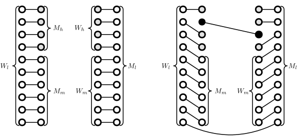
Figure 1: The (unique) stable marriages $\mu_{1}$ for disjoint (left) and $\mu_{0}$ for uniquely-intersecting (right) instances of the preferences described in Section 5.1.1.

Proof.

Let $\mu$ be a stable marriage; we will show that $\mu=\mu_{1}$. We first argue that every high and mid participant is married to a low participant in $\mu$. Suppose to the contrary that some $w=w_{i}$ for $i\leq n/2$ is married to some $m=m_{j}$ with $j\leq n/2$ in $\mu$. By the definition of the preferences and the assumption that $\operatorname{DISJ}(\bar{x},\bar{y})=1$, at least one of $w$ and $m$ prefers every low participant over their spouse. Assume without loss of generality that $w$ prefers all $m^{\prime}=m_{j^{\prime}}$ with $j^{\prime}>n/2$ over $m$. That is, $w$ prefers all low men over her spouse $m$. Since $w$ is married to a medium or high man, there must be some low man $m^{\prime}$ that is married to a low woman $w^{\prime}$. But $m^{\prime}$ prefers all high and medium women over $w^{\prime}$. In particular, he prefers $w$ over $w^{\prime}$. Therefore, $(w,m^{\prime})$ is a blocking pair, so $\mu$ is not stable. Thus any stable marriage must marry low participants to mid or high participants and vice versa.

Now we argue that if $(w_{i},m_{j+n/2})\in\mu$, then we must have $i=j$. The argument for pairs $(w_{i+n/2},m_{j})$ is identical. Suppose that $(w_{i},m_{j+n/2})\in\mu$ with $i<j$. Then there is some $j^{\prime}<j$ such that $m^{\prime}=m_{j^{\prime}+n/2}$ is married to $w^{\prime}=w_{i^{\prime}}$ with $i^{\prime}>i$. But then $(w_{i},m^{\prime})$ mutually prefer each other, contradicting the stability of $\mu$. We arrive at a similar contradiction if $i>j$, hence we must have $i=j$, as desired. ∎

Lemma 5.2.

Suppose we have a stable marriage instance with preferences described above corresponding to $\operatorname{DISJ}(\bar{x},\bar{y})=0$, with $\bar{x}$ and $\bar{y}$ uniquely intersecting. Let $x^{\alpha}_{\beta}=y^{\alpha}_{\beta}=1$ be the uniquely-intersecting entry of $\bar{x},\bar{y}$. In this case, there exists a unique stable marriage $\mu_{0}$ given by (see the right side of Figure 1)

$$\mu_{0}=\, \left\{(w_{\alpha},m_{\beta})\right\}\cup\left\{(w_{i},m_{i+n/2})\,\middle|\,i<\alpha\right\}$$

$$\cup\left\{(w_{i+n/2},m_{i})\,\middle|\,i<\beta\right\}$$

$$\cup\left\{(w_{i},m_{i+n/2-1}),\alpha<i\leq n/2\right\}$$

$$\cup\left\{(w_{i+n/2-1},m_{i}),\beta<i\leq n/2\right\}\cup\left\{(w_{n},m_{n})\right\}.$$

Proof.

We first argue that $(w_{\alpha},m_{\beta})\in\mu$ for any stable marriage $\mu$ for the preferences described above. Since $\mu$ is stable, if $(m_{\alpha},w_{\beta})\notin\mu$, then at least one of $w_{\alpha}$ and $m_{\beta}$, say $w_{\alpha}$, must be married to someone she prefers over $m_{\beta}$. From $w_{\alpha}$’s preferences, this implies that $(w_{\alpha},m)\in\mu$ for some $m=m_{j}$ with $j<\beta$ for which $x^{\alpha}_{j}=1$. Since the instance of $\operatorname{DISJ}$ is uniquely intersecting, we must have $y^{\alpha}_{j}=0$. Thus $m$ prefers all low women over $w_{\alpha}$. Since at most $n/2-1$ medium and high men are married to low women (indeed $m$ is a high man married to a high woman) and there are $n/2$ low women, some low woman $w$ is married to a low man. But then $w$ and $m$ mutually prefer each other, hence forming a blocking pair. Thus, we must have $(w_{\alpha},m_{\beta})\in\mu$.

The remainder of the proof of the lemma is analogous to the proof of Lemma 5.1 if we remove $w_{\alpha}$ and $m_{\beta}$ from all the participants’ preferences. ∎

Lemma 5.3.

The marriages $\mu_{0}$ and $\mu_{1}$ from the previous two lemmas satisfy $d(\mu_{0},\mu_{1})\geq(1-\delta)n.$

Proof.

This follows from the following two observations:

1. All mid women and men $M_{m}\cup W_{m}$ have different spouses in $\mu_{0}$ and $\mu_{1}$.

2. No mid women are married to mid men in either $\mu_{0}$ or $\mu_{1}$.

From these facts, we can conclude that $d(\mu_{0},\mu_{1})=n-\left|\mu_{0}\cap\mu_{1}\right|\geq\left|W_{m}\right|+\left|M_{m}\right|=(1-\delta)n.$ ∎

5.2 Derivation of Main results

In this section we use the construction of Section 5.1 to prove Theorems 3.1 and 3.2 from Section 3.

Proof of Theorem 3.1.

Suppose that $\Pi$ is a randomized communication protocol (between Alice and Bob) that outputs a $(1-\varepsilon)$-stable marriage $\mu$ using $B$ bits of communication. As $\varepsilon<1/2$, there exists $\delta$ sufficiently small such that $\varepsilon<(1-\delta)/2$. Suppose $\Pi$ outputs a $(1-\varepsilon)$-stable marriage $\mu$ for the preferences described in Section 5.1.1. If $\operatorname{DISJ}(\bar{x},\bar{y})=1$, then by Lemma 5.1, $\mu_{1}$ is the unique stable marriage, so $d(\mu,\mu_{1})\leq\varepsilon n$.

Suppose $\operatorname{DISJ}(\bar{x},\bar{y})=0$. By Lemma 5.2, $\mu_{0}$ is the unique stable marriage, so $d(\mu,\mu_{0})\leq\varepsilon n<(1-\delta)n/2$. Applying Lemma 5.3 and the triangle inequality, we obtain $d(\mu_{1},\mu)>(1-\delta)n/2>\varepsilon n$. Thus, if $\operatorname{DISJ}(\bar{x},\bar{y})=1$, then $d(\mu,\mu_{1})<\varepsilon n$ and if $\operatorname{DISJ}(\bar{x},\bar{y})=0$, then $d(\mu,\mu_{1})>\varepsilon n$. Given $\mu$, Alice and Bob can compute $d(\mu,\mu_{1})$ without communication, so they can use $\Pi$ to determine the value of $\operatorname{DISJ}(\bar{x},\bar{y})$ using $B$ bits of communication. Thus, $B=\Omega(n^{2})$ by Theorem 2.4, as desired. ∎

Proof of Theorem 3.2.

For Part (a), suppose that $\Pi$ is a randomized communication protocol that determines whether a given marriage $\mu$ is stable or $\varepsilon$-unstable with respect to given preferences using $B$ bits of communication. As $\varepsilon<1$, there exists $\delta$ sufficiently small such that $1-\delta>\varepsilon$. Let $\mu_{1}$ be the marriage defined in Lemma 5.1; by that lemma, if $\operatorname{DISJ}(\bar{x},\bar{y})=1$, then $\mu_{1}$ is stable (with respect to the preferences described in Section 5.1.1). By Lemmas 5.2 and 5.3, if $\operatorname{DISJ}(\bar{x},\bar{y})=0$, then $\mu_{1}$ is $\varepsilon$-unstable. Thus, if $\Pi$ determines whether $\mu_{1}$ is stable or $\varepsilon$-unstable, then $\Pi$ also determines the value of $\operatorname{DISJ}(\bar{x},\bar{y})$, hence $B=\Omega(n^{2})$ by Theorem 2.4.

For Part (b), suppose that $\Pi$ is a randomized communication protocol that for a given pair $(w,m)$ determines whether $(w,m)\in\mu$ for some (every) stable marriage $\mu$ using $B$ bits of communication. Set $\delta=1$. By choosing preferences as in Section 5.1.1 and taking $(w,m)=(w_{n},m_{n})$, by Lemmas 5.1 and 5.2, $(w,m)$ is in some (equivalently every) stable marriage for the given preferences if and only if $\operatorname{DISJ}(\bar{x},\bar{y})=0$. Thus, once again by Theorem 2.4, $B=\Omega(n^{2})$.

Finally, for Part (c), suppose that $\Pi$ is a randomized communication protocol that outputs $\varepsilon n$ pairs contained in some (every) stable marriage using $B$ bits of communication. Choose preferences as described in the Section 5.1.1 with some $0<\delta<\varepsilon$, say $\delta=\varepsilon/2$. Recall from the proof of Lemma 5.3 that no participants in $W_{m}$ and $M_{m}$ are ever married to one another in a stable marriage. Therefore, since $\left|W_{m}\right|+\left|M_{m}\right|=(1-\delta)n>(1-\varepsilon)n$ and since $\Pi$ outputs $\varepsilon n$ pairs, we have that $\Pi$ must output some pair $(w,m)$ with $w\in W_{m}$ or $m\in M_{m}$. Recall from the proof of Lemma 5.3 that knowing the stable spouse of any participant in $W_{m}$ or $M_{m}$ reveals the value of $\operatorname{DISJ}(\bar{x},\bar{y})$. Thus, by Theorem 2.4, $B=\Omega(n^{2})$. ∎

6 Computing Distance to Stability

In this section, we describe an efficient method for computing the divorce distance to stability of a given marriage, $\mu$. Recall that the divorce distance to stability is given by

$$d(\mu)=\min_{\mu^{\prime}\in\mathcal{M}}d(\mu,\mu^{\prime})\quad\text{where}\quad d(\mu,\mu^{\prime})=n-\left|\mu\cap\mu^{\prime}\right|.$$

In fact, our algorithm solves the following general problem, which we believe may be of independent interest: given a marriage market $\bigl{(}W,M,P_{W},P_{M}\bigr{)}$ and an arbitrary marriage $\mu$, find a stable marriage $\mu^{\prime}$ that shares the greatest number of pairs with $\mu$. Since the set $\mathcal{M}$ of all stable marriages can be exponentially large [19, 17, 15], brute-force computation of $d(\mu)$ is infeasible. Fortunately, by exploiting the structure of $\mathcal{M}$, we are able to efficiently reduce the computation of $d(\mu)$ to a max-flow/min-cut problem of size quadratic in $n$. Thus, any number of efficient algorithms may be applied to compute $d(\mu)$.

6.1 The Rotation Poset and Digraph

Our exposition follows the work of Gusfield [14] and of Irving and Leather [17] (see also [15]). Let $\mu$ be a stable marriage. A rotation $\mathbfit{\rho}$ exposed by $\mathbfit{\mu}$ is a sequence of pairs $(w_{0},m_{0}),(w_{1},m_{1}),\ldots,\linebreak(w_{r-1},m_{r-1})\in\mu$ such that for each $i$, $w_{i+1}$ is the first woman on $m_{i}$’s preference list that prefers $m_{i}$ to her partner $m_{i+1}$ in $\mu$ (where addition is conducted modulo $r$). Given $\mu$ and $\rho$, we form a marriage called the elimination of $\mathbfit{\rho}$ from $\mathbfit{\mu}$, denoted $\mu/\rho$, which contains the pairs $(w_{1},m_{0}),(w_{2},m_{1}),\ldots,(w_{0},m_{r-1})$, in addition to all pairs from $\mu$ that are not part of the rotation $\rho$. It is straightforward to verify that $\mu/\rho$ is a stable marriage.

Let $\mu_{0}$ denote the $M$-optimal stable marriage (the marriage found by the Gale-Shapley algorithm). Irving and Leather [17] prove that every stable marriage can be obtained from $\mu_{0}$ by successively eliminating a unique set of rotations that appear in $\mu_{0}$ and subsequent stable marriages. Given a stable marriage $\mu$, let $S_{\mu}$ denote this unique set of rotations, which can be eliminated (starting at $\mu_{0}$) to obtain $\mu$. ($S_{\mu}$ may contain some rotations that are not exposed in $\mu_{0}$, but only in subsequent marriages.)

We denote the set of all rotations exposed in one or more stable marriages in $\mathcal{M}$ by $\Pi(\mathcal{M})$. We endow $\Pi(\mathcal{M})$ with a partial order $\prec$ where $\rho\prec\sigma$ if $\rho\in S_{\mu}$ for every $\mu\in\mathcal{M}$ in which $\sigma$ is exposed. In other words, $\rho\prec\sigma$ if whenever $\sigma$ is eliminated during the construction of a stable marriage by elimination from $\mu_{0}$, it is the case that $\rho$ has been eliminated before $\sigma$. A subset $S\subseteq\Pi(\mathcal{M})$ is (downward) closed if for all $\sigma\in S$ and $\rho\prec\sigma$, we have that $\rho\in S$. Irving and Leather prove the following remarkable correspondence between closed subsets of $\Pi(\mathcal{M})$ and stable marriages.

Theorem 6.1 (Irving and Leather [17]).

The map $\mu\mapsto S_{\mu}$ is a bijection between $\mathcal{M}$ and the set of closed subsets of $\Pi(\mathcal{M})$.

For algorithmic purposes, it is advantageous to have a sparse representation of the partial order $\prec$ on $\Pi(\mathcal{M})$, which preserves its closed subsets. To this end, Gusfield [14] proved the following theorem. For the remainder of this section, we use the standard notation $\tilde{\mathcal{O}}$ to suppress $\log n$ factors, which we find less interesting in the context of our discussion of time complexity in this section (in contrast to the discussion of communication and query complexity in the rest of this paper).

Theorem 6.2 (Gusfield [14]).

There exists a directed acyclic graph $G(\mathcal{M})$ with vertices $\Pi(\mathcal{M})$, called the rotation digraph, whose transitive closure is the partial order $\prec$ on $\Pi(\mathcal{M})$. (That is, a path from a vertex $\rho$ to a vertex $\sigma$ exists iff $\rho\prec\sigma$.) $G(\mathcal{M})$ can be computed from the full preferences of all participants in time $\tilde{\mathcal{O}}(n^{2})$. In particular, the edge and vertex sets of $G(\mathcal{M})$ both have cardinality $\mathcal{O}(n^{2})$.

6.2 Rotation Weights

In this section, we show how to assign weights to rotations $\rho\in\Pi(\mathcal{M})$ in such a way that $d(\mu,\mu^{\prime})$ can be computed directly from $d(\mu,\mu_{0})$ and $S_{\mu^{\prime}}$. Let $\rho$ be any rotation and $\mu^{\prime}$ a stable marriage in which $\rho$ is exposed. For any marriage $\mu$, we define the weight $\gamma$ of $\rho$ relative to $\mu$ by

$$\gamma_{\mu}(\rho)=\left|\mu\cap(\mu^{\prime}/\rho)\right|-\left|\mu\cap\mu^{\prime}\right|.$$

(The absence of $\mu^{\prime}$ from the notation $\gamma_{\mu}(\rho)$ becomes clear in Eq. 1 below.) That is, $\gamma_{\mu}(\rho)$ is the net change, following the elimination of $\rho$ from $\mu^{\prime}$, in the number of pairs contained in the intersection of $\mu$ and $\mu^{\prime}$. We note that $\gamma_{\mu}(\rho)$ can be computed directly from $\rho$ (without being given an explicit stable marriage $\mu^{\prime}$ which exposes $\rho$). Specifically, letting $\rho^{\prime}=\left\{(w_{1},m_{0}),(w_{2},m_{1}),\ldots,(w_{0},m_{r-1})\right\}$ be the set of pairs replacing $\rho$ when eliminating $\rho$ from any stable marriage, we have

$$\gamma_{\mu}(\rho)=\left|\mu\cap\rho^{\prime}\right|-\left|\mu\cap\rho\right|.$$ (1)

Lemma 6.1.

For any marriage $\mu$ and stable marriage $\mu^{\prime}\in\mathcal{M}$,

$$\left|\mu\cap\mu^{\prime}\right|=\left|\mu\cap\mu_{0}\right|+\sum_{\rho\in S_{\mu^{\prime}}}\gamma_{\mu}(\rho),$$

where $\mu_{0}$ is the $M$-optimal stable marriage.

Proof.

We argue by induction on $\left|S_{\mu^{\prime}}\right|$. If $S_{\mu^{\prime}}=\varnothing$, then $\mu^{\prime}=\mu_{0}$, so the result is immediate. Suppose the claim is true for $\mu^{\prime}$ and $\sigma$ is a rotation exposed in $\mu^{\prime}$, then by the induction hypothesis and by definition of $\gamma_{\mu}(\sigma)$,

$$\left|\mu\cap(\mu^{\prime}/\sigma)\right|=\left|\mu\cap\mu^{\prime}\right|+\bigl{(}\left|\mu\cap(\mu^{\prime}/\sigma)\right|-\left|\mu\cap\mu^{\prime}\right|\bigr{)}=\left|\mu\cap\mu_{0}\right|+\sum_{\rho\in S_{\mu^{\prime}}}\gamma_{\mu}(\rho)+\gamma_{\mu}(\sigma),$$

which gives the desired result. ∎

Applying Lemma 6.1 and Theorem 6.1, we obtain the following result.

Theorem 6.3.

Let $\mu$ be a marriage. Then

$$d(\mu)=d(\mu,\mu_{0})-\max_{S}\sum_{\rho\in S}\gamma_{\mu}(\rho),$$

where the maximum is taken over closed subsets $S\subseteq\Pi(\mathcal{M})$ (and where $\mu_{0}$ is the $M$-optimal stable marriage).

Proof.

By Lemma 6.1, for any stable marriage $\mu^{\prime}$,

$$d(\mu,\mu^{\prime})=n-\left|\mu\cap\mu^{\prime}\right|=n-\left|\mu\cap\mu_{0}\right|-\sum_{\rho\in S_{\mu^{\prime}}}\gamma_{\mu}(\rho)=d(\mu,\mu_{0})-\sum_{\rho\in S_{\mu^{\prime}}}\gamma_{\mu}(\rho).$$

By Theorem 6.1, $\mu^{\prime}\mapsto S_{\mu^{\prime}}$ is a bijection onto the set of closed subsets of $\Pi(\mathcal{M})$. Thus,

$$d(\mu)=\min_{\mu^{\prime}\in\mathcal{M}}d(\mu,\mu^{\prime})=d(\mu,\mu_{0})-\max_{S}\sum_{\rho\in S}\gamma_{\mu}(\rho),$$

as desired. ∎

6.3 Reduction to Max-Flow/Min-Cut

We now wish to apply Theorems 6.2 and 6.3 to efficiently calculate $d(\mu)$. The divorce distance $d(\mu,\mu_{0})$ can easily be computed in $\tilde{\mathcal{O}}(n^{2})$ time by using the Gale-Shapley algorithm to compute $\mu_{0}$. Since the partial order $\prec$ on $\Pi(\mathcal{M})$ is the transitive closure of $G(\mathcal{M})$ (where $G(\mathcal{M})$ is the rotation digraph described in Theorem 6.2), the closed subsets of $\prec$ are precisely the (downward) closed subsets (vertex sets with no incoming edges) of $G(\mathcal{M})$, and so to compute $d(\mu)$ it suffices to maximize $\sum_{\rho\in S}\gamma_{\mu}(\rho)$ over closed subsets $S$ of $G(\mathcal{M})$. Thus, we have reduced the problem of computing $d(\mu)$ to finding a maximum closed subset (i.e. maximum-weight vertex set with no incoming edges) in a directed acyclic graph. This problem is well studied, in particular for its applications to open-pit mining (see, e.g. [27, 16]). For completeness and due to some differences in terminology between this paper and that of Picard [27], we briefly describe the application to our specific maximum closed subset problem of Picard’s [27] efficient reduction of maximum closed subset to max-flow/min-cut.

Denote the vertex and edge sets of $G(\mathcal{M})$ by $V=\Pi(\mathcal{M})$ and $E$ respectively. Let

$$V^{+}=\left\{\rho\in V\,\middle|\,\gamma_{\mu}(\rho)\geq 0\right\}\quad\text{and}\quad V^{-}=\left\{\rho\in V\,\middle|\,\gamma_{\mu}(\rho)<0\right\}.$$

We add a source vertex $s$ and a sink vertex $t$ to $G(\mathcal{M})$ to form a new $st$-graph $\tilde{G}=(\tilde{V},\tilde{E})$ where $\tilde{V}=V\cup\left\{s,t\right\}$ and

$$\tilde{E}~{}=~{}E~{}\cup~{}\left\{(s,\rho)\,\middle|\,\rho\in V^{-}\right\}~{}\cup~{}\left\{(\rho,t)\,\middle|\,\rho\in V^{+}\right\}.$$

We assign nonnegative capacity $c(u,v)$ to each edge $(u,v)\in\tilde{E}$ by

$$c(u,v)=\begin{cases}\infty&(u,v)\in E,\\ \gamma_{\mu}(\rho)&(u,v)=(\rho,t),\\ -\gamma_{\mu}(\rho)&(u,v)=(s,\rho).\end{cases}$$

Theorem 6.4 (Picard [27]).

The sink set (i.e. the set of vertices on the same side as the sink $t$) of a minimum $st$-cut in $\tilde{G}$ is a maximum closed subset in $G(\mathcal{M})$.

In light of Theorem 6.4, we can reduce the computation of $d(\mu)$ to known efficient algorithms for max-flow/min-cut. We summarize the procedure as follows.

Algorithm 1 $\mathrm{DivorceDistance}(\mu,P_{W},P_{M})$ — compute $d(\mu)$ with respect to preferences $P_{W},P_{M}$.

1. Use the Gale-Shapley algorithm to compute $\mu_{0}$ and compute $d(\mu,\mu_{0})=n-\left|\mu\cap\mu_{0}\right|$.

2. Construct the rotation digraph $G(\mathcal{M})$ and the related graph $\tilde{G}$.

3. Compute the weights in $\tilde{G}$ by computing $\gamma_{\mu}(\rho)$ for each rotation $\rho\in G(\mathcal{M})$, using Eq. (1).

4. Find a minimum $st$-cut in $\tilde{G}$, and let $S$ be the sink set in the cut.

5. Return $d(\mu,\mu_{0})-\sum_{\rho\in S}\gamma_{\mu}(\rho)$.

Theorem 6.5.

Given a marriage market $\bigl{(}W,M,P_{W},P_{M}\bigr{)}$ and a marriage $\mu$, running the procedure $\mathrm{DivorceDistance}(\mu,P_{W},P_{M})$ computes the divorce distance to stability $d(\mu)$ in time $\tilde{\mathcal{O}}(n^{4})$.

We remark that since $(P_{W},P_{M})$ has size $\tilde{\Theta}(n^{2})$, the runtime of $\mathrm{DivorceDistance}$ is nearly quadratic in the input size.

Proof of Theorem 6.5.

The correctness of $\mathrm{DivorceDistance}(\mu,P_{W},P_{M})$ follows immediately from Theorems 6.3 and 6.4. We analyze the runtime as follows. Step 1 can be computed in time $\tilde{\mathcal{O}}(n^{2})$ using the Gale-Shapley algorithm and brute force computation of $d(\mu,\mu_{0})$. For Step 2, by Theorem 6.2, $G(\mathcal{M})$ (and hence $\tilde{G}$) can also be computed in time $\tilde{\mathcal{O}}(n^{2})$. The weights in Step 3 can be computed in linear time for each rotation, so computing all the weights can be accomplished in time $\tilde{\mathcal{O}}(n^{3})$. For Step 4, the min-cut can be computed in time $\tilde{\mathcal{O}}\bigl{(}|\tilde{E}||\tilde{V}|\bigr{)}=\tilde{\mathcal{O}}(n^{4})$ using, for example, Hochbaum’s algorithm [16]. ∎

We remark that since Algorithm 1 finds both $\mu_{0}$ and $S=S_{\mu^{\prime}}$ for a stable marriage $\mu^{\prime}$ closest to $\mu$, it is a trivial task, which does not increase the asymptotic runtime complexity of Algorithm 1, to also compute $\mu^{\prime}$ in addition to computing $d(\mu)=d(\mu,\mu^{\prime})$.

7 Commentary and Open Problems

A number of recent papers [2, 12] have touched on various aspects of the amorphic question of “how much do the preferences of the women in the Gale-Shapley algorithm affect the produced ($M$-optimal) stable marriage.” The fact that we prove our lower-bound result in a strong two-sided communication model (and not a weaker $2n$-sided communication model or an even-weaker query model) allows our results to also be viewed in the context of this line of research. Our communication lower bounds show that a significant amount of information about the preferences of the women is indeed needed in order to deduce the $M$-optimal stable marriage, as well as for solving any of the other problems described in Corollary 3.2.

One qualitative feature of of the Gale-Shapley algorithm is that a single proposal at any point can precipitate a cascade of rejections that affects a large portion of the population. Thus, it is impossible for participants to know if their current partner is their final partner until the algorithm has terminated. Our results imply that this feature is common to all stable marriage mechanisms that dynamically refine a marriage and converge to a stable marriage. Indeed, consider any stable marriage algorithm and arbitrarily divide it into a “first” stage and a “second” stage. A consequence of Corollary 3.1 along with our novel definition of divorce distance is that if the query complexity of the first stage is significantly lower than that of querying the entire input, then after the first stage a large fraction of the participants may not yet be married to their final spouses.

In many real-world marriage markets, centralized clearinghouses are employed to prevent undesirable outcomes [29, 31]. Specifically, these clearinghouses were implemented to avoid “unraveling” — wherein participants are incentivized to match extremely early — as well as instability. While unraveling is undesirable in its own right, the early binding commitments made in an unraveling market have been shown to have adverse effects [32, 21, 25, 10], presumably because the early matches are necessarily made with incomplete knowledge about the market. A consequence of Corollary 3.2 (specifically, of Part (c)) is that any marriage mechanism that allows even a small fraction of participants to match in early binding commitments (i.e. before essentially all of the preferences are queried) cannot generally produce a stable marriage. Thus the empirical phenomenon of instability in decentralized markets where early-accepted proposals are binding, which was observed in [29, 31], is not merely a feature of the particular marriage mechanisms that arose in practice, but is a general theoretical feature inherent in the stable marriage problem.

It is interesting to compare the $\Omega(n^{2})$ lower bound that is proved in this paper for the communication complexity of finding an approximately stable marriage to known complexity bounds for the problem of finding an approximately maximum-weight matching in a bipartite graph. Even though these two problems seem similar, the latter can be solved with $\mathcal{O}(n\log n)$ communication [7], i.e. with significantly less communication than many variants of the former. It is worthwhile to compare this surprising dissimilarity between these problems with a qualitatively similar message that emerges from a significantly different, recent line of work [22, 1], which shows that finding a Pareto-efficient perfect matching requires considerably less strategic reasoning than finding a stable marriage.

The classic Gale-Shapley algorithm [11] terminates after $\mathcal{O}(n^{2})$ steps, and each step consists of a message of $\mathcal{O}(\log n)$ bits. Thus, the Gale-Shapley algorithm provides a communication upper bound of $\mathcal{O}(n^{2}\log n)$ for the problem of finding a stable marriage. As mentioned in the introduction, our Theorem 3.1 matches this up to a logarithmic factor, but it is not immediately clear how to close this gap.

Open Problem 7.1.

What is the communication complexity of finding a stable marriage?

Our definition of $(1-\varepsilon)$-stability is nonstandard. A more common notion of approximate stability is that a marriage induce few (say, at most $\varepsilon n^{2}$) blocking pairs (see [9]). As shown in Propositions 2.1, the blocking-pairs notion of approximate stability is strictly coarser than ours. It is therefore natural to ask if the $\Omega(n^{2})$ communication lower bound of Theorem 3.1 holds as well with respect to the more challenging concept of blocking-pairs approximate stability.

Open Problem 7.2.

Is there a protocol $\Pi$ that computes a marriage with at most $\varepsilon n^{2}$ blocking pairs using $o(n^{2})$ communication?

Recently, Ostrovsky and Rosenbaum [26] showed that it is possible to find a marriage with $\varepsilon n^{2}$ blocking pairs for arbitrary $\varepsilon>0$ using $\mathcal{O}(1)$ communication rounds for a distributed model of computation. While their result does not imply anything nontrivial about the total communication, we believe their techniques may be relevant for finding $o(n^{2})$ communication protocols for blocking-pairs approximate stability (if such protocols exist). Interestingly, an analogue of Theorem 3.2(a) (or of Corollary 3.2(a)) does not hold for blocking-pairs approximate stability.

Theorem 7.1.

For every $\varepsilon\geq\delta>0$, there exists a randomized communication protocol $\Pi$ that determines whether a given marriage $\mu$ induces at least $\varepsilon n(n-1)$ blocking pairs or at most ${(\varepsilon-\delta)n(n-1)}$ blocking pairs using $\mathcal{O}(\log n)$ communication. In particular, $\Pi$ determines whether $\mu$ is stable or has $\varepsilon n(n-1)$ blocking pairs using $\mathcal{O}(\log n)$ communication.

Proof sketch..

Choose an unmarried pair $(w,m)$ uniformly at random from $W\times M$. If $m$ prefers $w$ over his spouse in $\mu$, the men query the women to see if $w$ also prefers $m$ over her spouse in $\mu$ using $\mathcal{O}(\log n)$ communication. The probability that $(w,m)$ is a blocking pair is precisely $\varepsilon^{\prime}$, where $\varepsilon^{\prime}$ is the fraction of blocking pairs in $\mu$. Repeat this procedure to estimate $\varepsilon^{\prime}$ to any desired accuracy in a bounded number of steps depending only on the desired accuracy. ∎

Theorem 3.2(c) shows that any protocol that produces a constant fraction of pairs in a stable marriage (regardless of which pairs are found) requires $\Omega(n^{2})$ communication. It would be interesting to improve this result (or find an efficient protocol) for finding even a single pair that appears in a stable marriage.

Open Problem 7.3.

What is the communication complexity of finding a single pair $(w,m)$ that appears in some/every stable marriage?

Finally, we notice that in contrast to Parts (a) and (c) of Theorem 3.2, our statement of Theorem 3.1 requires that $\varepsilon<1/2$. It is natural to ask what can be obtained regarding other values of $\varepsilon$.

Open Problem 7.4.

Fix $\frac{1}{2}\leq\varepsilon<1$. What is the communication complexity of finding a $(1-\varepsilon)$-stable marriage?

Appendix A Asymptotic Notation

Throughout this paper, we use standard computer-science asymptotic notation to describe the order of growth of single-dimensional functions of natural numbers. For example, for a positive function $f$, we write $f(n)=\mathcal{O}\bigl{(}g(n)\bigr{)}$ where $g$ is also a positive function (usually, one simple to write down), if there exist positive numbers $\overline{M}$ and $N$ such that $f(n)\leq\overline{M}\cdot g(n)$ for all $n>N$. (Equivalently and succinctly, we write $f=\mathcal{O}\bigl{(}g(n)\bigr{)}$ if $\lim\sup_{n\rightarrow\infty}\frac{f(n)}{g(n)}<\infty$.) Intuitively, one may find it helpful to read the notation $f=\mathcal{O}\bigl{(}g(n)\bigr{)}$ as $f\in\mathcal{O}(g)$, where $\mathcal{O}(g)$ is the class of functions whose order of growth (as $n$ grows large) is at most that of $g$. This notation allows for the simplification of the exposition of many results, where the order of magnitude of the result serves as the main message. For example, for a highly complex function $f$ that satisfies $f=\mathcal{O}\bigl{(}n^{2}\bigr{)}$ (that is, does not grow any faster than $g$, where $g(n)=n^{2}$ for all $n$), instead of specifying $f$ and saying that some algorithm takes at most $f$ steps, one could concisely say that this algorithm takes at most $\mathcal{O}(n^{2})$ steps, without the need to explicitly write down the complex function $f$. The following table summarizes this and other similar standard “order of growth” notation used throughout this paper.

Notation	Explicit Definition	Succinct Definition	Informal Meaning
$f=\mathcal{O}\bigl{(}g(n)\bigr{)}$	4cm$\exists\overline{M},N:\forall n>N:$
$f(n)\leq\overline{M}\cdot g(n)$	$\lim\sup_{n\rightarrow\infty}\frac{f(n)}{g(n)}<\infty$	$f$ grows at most as fast as $g$
$f=\Omega\bigl{(}g(n)\bigr{)}$	4cm$\exists\underline{M}>0,N:\forall n>N:$
$f(n)\geq\underline{M}\cdot g(n)$	$\lim\inf_{n\rightarrow\infty}\frac{f(n)}{g(n)}>0$	$f$ grows at least as fast as $g$
$f=\Theta\bigl{(}g(n)\bigr{)}$	4cm$\exists\underline{M}>0,\overline{M},N:\forall n>N:$
$\underline{M}\cdot g(n)\leq f(n)\leq\overline{M}\cdot g(n)$	3cm$f=\mathcal{O}\bigl{(}g(n)\bigr{)}$ &
$f=\Omega\bigl{(}g(n)\bigr{)}$	$f$ grows as fast as $g$
$f=o\bigl{(}g(n)\bigr{)}$	4cm$\forall\overline{M}>0:\exists N:\forall n>N:$
$f(n)\leq\overline{M}\cdot g(n)$	$\lim\sup_{n\rightarrow\infty}\frac{f(n)}{g(n)}=0$	$f$ grows slower than $g$
$f=\omega\bigl{(}g(n)\bigr{)}$	4cm$\forall\underline{M}:\exists N:\forall n>N:$
$f(n)\geq\underline{M}\cdot g(n)$	$\lim\inf_{n\rightarrow\infty}\frac{f(n)}{g(n)}=\infty$	$f$ grows faster than $g$

Appendix B Embedding Arbitrary Preferences into Complete Preferences

This section contains the remaining technical details needed to complete the direct proof that is given in Section 4 of our lower bound on the communication complexity of finding an exactly stable marriage.

Definition B.1 (Submarriage).

Let $W^{\prime}$ and $M^{\prime}$ be disjoint sets. A marriage $\mu$, between a subset $W$ of $W^{\prime}$ and a subset $M$ of $M^{\prime}$, is said to be a submarriage of a marriage $\mu^{\prime}$ between $W^{\prime}$ and $M^{\prime}$, if for every $w\in W$ and $m\in M$, we have $\mu^{\prime}(w)=m$ iff $\mu(w)=m$.

Lemma B.1 (Finding a Stable Marriage (Arbitrary Preferences) $\hookrightarrow$ Finding a Stable Marriage (Full Preferences)).

Let $n\in\mathbb{N}$, and let $W$, $W^{\prime}$, $M$ and $M^{\prime}$ be pairwise-disjoint sets, each of cardinality $n$. There exist functions $P_{W\cup W^{\prime}}:\mathcal{P}(W,M)\rightarrow\mbox{$\mathcal{F}(W\cup W^{\prime},M\cup M^{\prime})$}$ and $P_{M\cup M^{\prime}}:\mathcal{P}(M,W)\rightarrow\mbox{$\mathcal{F}(M\cup M^{\prime},W\cup W^{\prime})$}$ such that for every $P_{W}\in\mathcal{P}(W,M)$ and $P_{M}\in\mathcal{P}(M,W)$, and for every (possibly imperfect) marriage $\mu$ between $W$ and $M$, the following are equivalent.

• $\mu$ is stable with respect to $P_{W}$ and $P_{M}$.

• $\mu$ is a submarriage of some marriage between $W\cup W^{\prime}$ and $M\cup M^{\prime}$ that is stable with respect to $P_{W\cup W^{\prime}}(P_{W})$ and $P_{M\cup M^{\prime}}(P_{M})$.

Proof..

Denote $W\!=\!\{w_{1},\ldots,w_{n}\}$, $M\!=\!\{m_{1},\ldots,m_{n}\}$, $W^{\prime}\!=\!\{w^{\prime}_{1},\ldots,w^{\prime}_{n}\}$, and $M^{\prime}\!=\!\{m^{\prime}_{1},\ldots,m^{\prime}_{n}\}$.

To define $P_{W\cup W^{\prime}}(P_{W})$, for every $i$ we define the preference list of $w_{i}$ to consist of her preference list in $P_{W}$ (in the same order), followed by $m^{\prime}_{i}$, followed by all other men in arbitrary order; we define the preference list of $w^{\prime}_{i}$ to consist of $m_{i}$, followed by all other men in arbitrary order. Similarly, to define $P_{M\cup M^{\prime}}(P_{M})$, for every $j$ we define the preference list of $m_{j}$ to consist of his preference list in $P_{M}$ (in the same order), followed by $w^{\prime}_{j}$, followed by all other women in arbitrary order; we define the preference list of $m^{\prime}_{j}$ to consist of $w_{j}$, followed by all other women in arbitrary order.

It is straightforward to verify that the lemma holds with respect to these definitions of $P_{W\cup W^{\prime}}$ and $P_{M\cup M^{\prime}}$; the details are left to the reader. ∎

Remark B.1.

It is straightforward to embed the problem of finding a stable marriage with respect to full preference lists in that of finding a stable marriage with respect to arbitrary preference lists, as the former is a special case of the latter.

Appendix C Determining the Marital Status of
a Given Couple or Participant

In this appendix, we give an alternate proof of Part (b) of Theorem 3.2 that uses the construction of Section 4. We prove Theorem 3.2(b) once again using Theorem 2.4, by embedding disjointness (without assuming unique intersection) in both problems. We embed disjointness via an intermediate problem of determining whether a given participant is single (i.e. not married to anyone) in some stable marriage, given profiles of arbitrary (i.e. not necessarily full) preference lists. We therefore obtain the same lower bounds for this natural problem as well.

Lemma C.1 (Disjointness $\hookrightarrow$ Is Participant Single?).

Let $n\in\mathbb{N}$, let $W$ and $M$ be disjoint sets such that $|W|=|M|=2n$, and let $p\in W\cup M$. There exist functions $P_{W}:\{0,1\}^{[n]^{\underline{2}}}\rightarrow\mathcal{P}(W,M)$ and $P_{M}:\{0,1\}^{[n]^{\underline{2}}}\rightarrow\mathcal{P}(M,W)$ such that for every $\bar{x}=(x^{i}_{j})_{(i,j)\in[n]^{\underline{2}}}\in\{0,1\}^{[n]^{\underline{2}}}$ and $\bar{y}=(y^{i}_{j})_{(i,j)\in[n]^{\underline{2}}}\in\{0,1\}^{[n]^{\underline{2}}}$, the following are equivalent.

• $p$ is single in some stable marriage with respect to $P_{W}(\bar{x})$ and $P_{M}(\bar{y})$.

• $\operatorname{DISJ}(\bar{x},\bar{y})\neq 0$.

Proof.

Assume without loss of generality that $p\in W$ and denote $w=p$. Denote $W=\{w_{1},\ldots,w_{n},\allowbreak w,w^{\prime}_{2},w^{\prime}_{3},\ldots,w^{\prime}_{n}\}$ and $M=\{m_{1},\ldots,m_{n},m^{\prime}_{1},\ldots,m^{\prime}_{n}\}$.

To define $P_{W}(\bar{x})$, for every $i$ we define the preference list of $w_{i}$ to consist of all $m_{j}$ such that $x^{i}_{j}=1$, in arbitrary order (say, sorted by $j$), followed by $m^{\prime}_{i}$ (with all other men absent). We define the preference list of $w$ to consist of all $m^{\prime}_{j}$, in arbitrary order (say, sorted by $j$), with all other men absent. We define the preference list of every $w^{\prime}_{i}$ to be empty (these women can be ignored, and are defined purely for aesthetic reasons — so that $W$ and $M$ be of equal cardinality). To define $P_{M}(\bar{y})$, for every $j$ we define the preference list of $m_{j}$ to consist of all $w_{i}$ such that $y^{i}_{j}=1$, in arbitrary order (say, sorted by $i$), with all other women absent. For every $j$ we define the preference list of $m^{\prime}_{j}$ to consist of $w_{j}$, followed by $w$ (with all other women absent).

Let $\mu_{\mathrm{id}}^{\prime}$ be the marriage in which $w_{i}$ is married to $m^{\prime}_{i}$ for every $i$, and in which all other participants are single. We first show that $\operatorname{DISJ}(\bar{x},\bar{y})\neq 0$ iff $\mu_{\mathrm{id}}^{\prime}$ is stable, and then show that $\mu_{\mathrm{id}}^{\prime}$ is stable iff $w=p$ is single in some stable marriage; we commence with the former.

We begin by noting that every participant that is married in $\mu_{\mathrm{id}}^{\prime}$ is married to someone on their preference list; therefore, $\mu_{\mathrm{id}}^{\prime}$ is stable iff no pair would rather deviate. Obviously, no $w^{\prime}_{i}$ would rather deviate with anyone. Furthermore, while $w$ would rather deviate with any $m^{\prime}_{j}$, these are all married to their top choices, and so none of them would deviate with $w$. Since for every $i$, the preference list of $w_{i}$ consists of $m^{\prime}_{i}$ and of a subset of $\{m_{j}\}_{j\neq i}$, we therefore have that $\mu_{\mathrm{id}}^{\prime}$ is unstable iff there exists $(i,j)\in[n]^{\underline{2}}$ such that both $m_{j}\succ_{w_{i}}m^{\prime}_{i}$ and $w_{i}$ is on the preference list of $m_{j}$. Similarly to the proof of Lemma 4.2, this holds precisely if there exists $(i,j)\in[n]^{\underline{2}}$ such that $x^{i}_{j}=1$ and $y^{i}_{j}=1$, which holds iff $\operatorname{DISJ}(\bar{x},\bar{y})=0$.

We complete the proof by showing that $\mu_{\mathrm{id}}^{\prime}$ is stable iff $w=p$ is single in some stable marriage. The first direction follows immediately from the fact that $w$ is single in $\mu_{\mathrm{id}}^{\prime}$. For the second direction, assume that there exists a stable marriage $\mu$ in which $w$ is single. By stability of $\mu$ and since all men on the preference list of $w$ have $w$ on their preference list, all such men are married in $\mu$ and prefer their spouses over $w$. Therefore, for every $j$, we have that $m^{\prime}_{j}$ is married to $w_{j}$ in $\mu$. By stability of $\mu$, every $w^{\prime}_{i}$ is single in $\mu$. As $\mu$ and $\mu_{\mathrm{id}}^{\prime}$ coincide on all women, we have that $\mu=\mu_{\mathrm{id}}^{\prime}$. Therefore, $\mu_{\mathrm{id}}^{\prime}=\mu$ is stable and the proof is complete. ∎

Corollary C.1 (Complexity of Determining the Marital Status of a Given Participant).

The lower bounds of Theorem 3.2 and Corollary 3.2 apply also to the problem of determining whether a given participant $p\in W\cup M$ is single in some (equivalently, in every) stable marriage, where $P_{W}\in\mathcal{P}(W,M)$ and $P_{M}\in\mathcal{P}(M,W)$ are arbitrary (i.e. not necessarily full) preference lists.

Lemma C.2 (Is Participant Single? $\hookrightarrow$ Is Couple Sometimes/Always Married?).

Let $n\in\mathbb{N}$, and let $W$, $W^{\prime}$, $M$ and $M^{\prime}$ be pairwise-disjoint sets, each of cardinality $n$; let $w\in W$ and $m^{\prime}\in M^{\prime}$. There exist functions $P_{W\cup W^{\prime}}:\mathcal{P}(W,M)\rightarrow\mbox{$\mathcal{F}(W\cup W^{\prime},M\cup M^{\prime})$}$ and $P_{M\cup M^{\prime}}:\mathcal{P}(M,W)\rightarrow\mbox{$\mathcal{F}(M\cup M^{\prime},W\cup W^{\prime})$}$ such that for every $P_{W}\in\mathcal{P}(W,M)$ and $P_{M}\in\mathcal{P}(M,W)$, the following are equivalent.

• $w$ is single in some marriage between $W$ and $M$ that is stable with respect to $P_{W}$ and $P_{M}$.

• $w$ and $m^{\prime}$ are married in some marriage between $W\cup W^{\prime}$ and $M\cup M^{\prime}$ that is stable with respect to $P_{W\cup W^{\prime}}(P_{W})$ and $P_{M\cup M^{\prime}}(P_{M})$.

• $w$ and $m^{\prime}$ are married in every marriage between $W\cup W^{\prime}$ and $M\cup M^{\prime}$ that is stable with respect to $P_{W\cup W^{\prime}}(P_{W})$ and $P_{M\cup M^{\prime}}(P_{M})$.

Proof.

The proof is similar to that of Lemma B.1. Denote $W=\{w_{1}=w,w_{2},\ldots,w_{n}\}$, $M=\{m_{1},\ldots,m_{n}\}$, $W^{\prime}=\{w^{\prime}_{1},\ldots,w^{\prime}_{n}\}$, and $M^{\prime}=\{m^{\prime}_{1}=m^{\prime},m^{\prime}_{2},\ldots,m^{\prime}_{n}\}$.

To define $P_{W\cup W^{\prime}}(P_{W})$, for every $i$ we define the preference list of $w_{i}$ to consist of her preference list in $P_{W}$ (in the same order), followed by $m^{\prime}_{i}$, followed by all other men in arbitrary order; we define the preference list of $w^{\prime}_{i}$ to consist of $m_{i}$, followed by all other men in arbitrary order. Similarly, to define $P_{M\cup M^{\prime}}(P_{M})$, for every $j$ we define the preference list of $m_{j}$ to consist of his preference list in $P_{M}$ (in the same order), followed by $w^{\prime}_{j}$, followed by all other women in arbitrary order; we define the preference list of $m^{\prime}_{j}$ to consist of $w_{j}$, followed by all other women in arbitrary order.

Similarly to the proof of Lemma B.1, we have that $w$ is single in some marriage $\mu$ between $W$ and $M$ that is stable with respect to $P_{W}$ and $P_{M}$ iff $w$ and $m^{\prime}$ are married in some marriage (a corresponding “supermarriage” of $\mu$) between $W\cup W^{\prime}$ and $M\cup M^{\prime}$ that is stable with respect to $P_{W\cup W^{\prime}}(P_{W})$ and $P_{M\cup M^{\prime}}(P_{M})$. Additionally, by Theorem 2.3 (in conjunction with Theorem 2.1), we have: $w$ is single in some marriage between $W$ and $M$ that is stable with respect to $P_{W}$ and $P_{M}$ $\Longleftrightarrow$ $w$ is single in every marriage between $W$ and $M$ that is stable with respect to $P_{W}$ and $P_{M}$ $\Longleftrightarrow$ $w$ and $m^{\prime}$ are married in every marriage between $W\cup W^{\prime}$ and $M\cup M^{\prime}$ that is stable with respect to $P_{W\cup W^{\prime}}(P_{W})$ and $P_{M\cup M^{\prime}}(P_{M})$. ∎

Appendix D Verifying the Output of a Given Stable Marriage Mechanism

As noted in Section 3, while our lower bound for verifying the stability of a given marriage is tight, we do now know whether our lower bound for finding a stable marriage is tight as well. We note that we do not even know a tight lower bound for verifying whether a given marriage is the $M$-optimal stable marriage.

Open Problem D.1.

What is the worst-case complexity of verifying whether a given marriage is the $M$-optimal stable marriage?

As in the case of Open Problem 1.1, we do not have any $o(n^{2}\log n)$ algorithm for verification of the $M$-optimal stable marriage, even randomized and even in the strong two-party communication model, nor do we have any $\omega(n^{2})$ lower bound, even for deterministic algorithms and even in the simple comparison model.

In this section, we the derive a $\Omega(n^{2})$ lower bound for verification of the $M$-optimal stable marriage. In fact, we show this lower bound not only for verifying the $M$-optimal stable marriage, but also for verifying the output of any other stable marriage mechanism.

Definition D.1 (Stable Marriage Mechanism).

Let $n\in\mathbb{N}$, let $W$ and $M$ be disjoint sets such that $|W|=|M|=n$. A stable marriage mechanism is a function $f$ from $\mathcal{F}(W,M)\times\mathcal{F}(M,W)$ to the set of perfect marriages between $W$ and $M$, such that for every $P_{W}\in\mathcal{F}(W,M)$ and $P_{M}\in\mathcal{F}(M,W)$, the marriage $f(P_{W},P_{M})$ is stable with respect to $P_{W}$ and $P_{M}$.

Example D.1 ($M$-Optimal Stable Marriage Mechanism).

The function $f_{\mbox{\scriptsize$M$-Opt}}$, defined such that $f_{\mbox{\scriptsize$M$-Opt}}(P_{W},P_{M})$ is the $M$-optimal stable marriage with respect to $P_{W}$ and $P_{M}$, is a well-defined stable marriage mechanism by Theorem 2.1.

Corollary D.1 (Complexity of Computing the Output of a Given Stable Marriage Mechanism).

By Theorem 3.1, we have that for every stable marriage mechanism $f$, the worst-case randomized query complexity (as defined in Corollary 3.1) as well as the worst-case communication complexity of computing $f$ is $\Omega(n^{2})$.

Theorem D.1 (Complexity of Verifying the Output of a Given Stable Marriage Mechanism).

Let $n\in\mathbb{N}$, let $W$ and $M$ be disjoint sets such that $|W|=|M|=n$, fix a stable marriage mechanism $f$ and let $P_{W}\in\mathcal{F}(W,M)$ and $P_{M}\in\mathcal{F}(M,W)$. Let $\mu_{\mathrm{id}}$ be the perfect marriage in which $w_{i}$ is married to $m_{i}$ for every $i$. The worst-case randomized query complexity, as well as the worst-case randomized communication complexity, of determining whether $f(P_{W},P_{M})=\mu_{\mathrm{id}}$ is $\Omega(n^{2})$.

Theorem D.1 may be proven either via a direct application of the machinery of Section 5, or using the machinery of Section 4, with Lemma B.1 replaced by the following lemma.

Lemma D.1.

Let $n\in\mathbb{N}$, and let $W=\{w_{1},\ldots,w_{n}\}$, $M=\{m_{1},\ldots,m_{n}\}$, $W^{\prime}=\{w^{\prime}_{1},\ldots,w^{\prime}_{n}\}$ and $M^{\prime}=\{m^{\prime}_{1},\ldots,m^{\prime}_{n}\}$ be pairwise-disjoint sets, each of cardinality $n$. Let $\mu_{\mathrm{id}}$ be the perfect marriage between $W$ and $M$ in which $w_{i}$ is married to $m_{i}$ for every $i$, and let $\mu_{\mathrm{id}}^{\prime}$ be the perfect marriage between $W\cup W^{\prime}$ and $M\cup M^{\prime}$ in which for every $i$, both $w_{i}$ is married to $m_{i}$ and $w^{\prime}_{i}$ is married to $m^{\prime}_{i}$. There exist functions $P_{W\cup W^{\prime}}:\mathcal{P}(W,M)\rightarrow\mbox{$\mathcal{F}(W\cup W^{\prime},M\cup M^{\prime})$}$ and $P_{M\cup M^{\prime}}:\mathcal{P}(M,W)\rightarrow\mbox{$\mathcal{F}(M\cup M^{\prime},W\cup W^{\prime})$}$ such that for every $P_{W}\in\mathcal{P}(W,M)$ and $P_{M}\in\mathcal{P}(M,W)$, both of the following hold.

1. If $\mu_{\mathrm{id}}$ is the unique stable marriage with respect to $P_{W}$ and $P_{M}$, then $\mu_{\mathrm{id}}^{\prime}$ is the unique stable marriage with respect to $P_{W\cup W^{\prime}}(P_{W})$ and $P_{M\cup M^{\prime}}(P_{M})$.

2. If $\mu_{\mathrm{id}}$ is unstable with respect to $P_{W}$ and $P_{M}$, then $\mu_{\mathrm{id}}^{\prime}$ is unstable with respect to $P_{W\cup W^{\prime}}(P_{W})$ and $P_{M\cup M^{\prime}}(P_{M})$.

Proof.

We define $P_{W\cup W^{\prime}}(P_{W})$ and $P_{M\cup M^{\prime}}(P_{M})$ as in Lemma B.1, only with $M^{\prime}$ appearing sorted by $j$ (as opposed to in arbitrary order) on the preference lists of $W^{\prime}$, and with $W^{\prime}$ appearing sorted by $i$ (as opposed to in arbitrary order) on the preference lists of $M^{\prime}$. By Lemma B.1, we have both that b. holds, and that if $\mu_{\mathrm{id}}$ is the unique stable marriage with respect to $P_{W}$ and $P_{M}$, then it is a submarriage of every marriage that is stable with respect to $P_{W\cup W^{\prime}}(P_{W})$ and $P_{M\cup M^{\prime}}(P_{M})$; it is straightforward to show that every “supermarriage” of $\mu_{\mathrm{id}}$, apart from $\mu_{\mathrm{id}}^{\prime}$, is unstable, thus proving a. as well. ∎

Open Problem D.2.

Is there a stable marriage mechanism whose worst-case output verification complexity is $\Theta(n^{2})$? Which stable marriage mechanisms have the lowest asymptotic worst-case output verification complexity?

Appendix E Nondeterminism

All the lower bounds in this paper are based upon reductions to the well-studied communication complexity of the disjointness function. Since the disjointness function also has $\Theta(n)$ nondeterministic communication complexity [20], it follows that all our lower bounds apply not only to randomized communication complexity, but also to nondeterministic communication complexity. For nondeterministic communication complexity, the $\Omega(n^{2})$ lower bound for finding a stable marriage is in fact tight (and so still is the $\Omega(n^{2})$ bound for verification of stability).

For the decision problem of verifying the stability of a given marriage, the co-nondeterministic communication complexity may be easily seen to be $\Theta(\log n)$. In contrast, we note that the proof of Theorem 3.2(b) may be easily adapted to show a $\Omega(n^{2})$ lower bound also for the co-nondeterministic communication complexities of determining the marital status of a given couple.

Theorem E.1 (Nondeterministic Communication Complexity of Determining the Marital Status of a Given Couple).

In the notation of Theorem 3.2(b), both the nondeterministic and co-nondeterministic communication complexities of determining whether $w$ and $m$ are married in some/every stable marriage are $\Omega(n^{2})$.

For completeness, we show this lower bound also for the nondeterministic and co-nondeterministic communication complexities of the intermediate problem of determining whether a given participant is single, which we presented in Appendix C. (This proof also yields Theorem E.1 using the tools of that appendix and of Section 4.) These lower bounds follow from the results of Appendix C in conjunction with the following lemma.

Lemma E.1 (Is Participant Single? $\hookrightarrow\lnot$ Is Participant Single?).

Let $n\in\mathbb{N}$, let $W$ and $M$ be sets such that $|W|=|M|=n$, and let $w^{\prime}$ and $m^{\prime}$ such that $W$, $M$, $\{w^{\prime}\}$ and $\{m^{\prime}\}$ are pairwise disjoint; let $w\in W$. There exist functions $P_{W\cup\{w^{\prime}\}}:\mathcal{P}(W,M)\rightarrow\mbox{$\mathcal{P}(W\cup\{w^{\prime}\},M\cup\{m^{\prime}\})$}$ and $P_{M\cup\{m^{\prime}\}}:\mathcal{P}(M,W)\rightarrow\mbox{$\mathcal{P}(M\cup\{m^{\prime}\},W\cup\{w^{\prime}\})$}$ such that for every $P_{W}\in\mathcal{P}(W,M)$ and $P_{M}\in\mathcal{P}(M,W)$, the following are equivalent.

• $w$ is single in some marriage between $W$ and $M$ that is stable with respect to $P_{W}$ and $P_{M}$.

• $m^{\prime}$ is married in every marriage between $W\cup\{w^{\prime}\}$ and $M\cup\{m^{\prime}\}$ that is stable with respect to $P_{W\cup\{w^{\prime}\}}(P_{W})$ and $P_{M\cup\{m^{\prime}\}}(P_{M})$.

Proof.

To define $P_{W\cup\{w^{\prime}\}}(P_{W})$, we define the preference list of $w$ as her preference list in $P_{W}$ (in the same order), followed by $m^{\prime}$; we define the preference list of every other woman in $W$ as her preference list in $P_{W}$ (in the same order and with $m^{\prime}$ absent), and define the preference list of $w^{\prime}$ to be empty (once again, $w^{\prime}$ can be ignored, and is defined purely for aesthetic reasons — so that $W\cup\{w^{\prime}\}$ and $M\cup\{m^{\prime}\}$ be of equal cardinality). To define $P_{M\cup\{m^{\prime}\}}(P_{M})$, we define the preference list of every man in $M$ as his preference list in $P_{M}$ (in the same order and with $w^{\prime}$ absent); we define the preference list of $m^{\prime}$ to consist solely of $w$.

Directly from definition of $P_{M\cup M^{\prime}}$ and $P_{W\cup W^{\prime}}$, we have that a natural bijection $\mu\mapsto\mu^{\prime}$ exists between stable marriages with respect to $P_{W}$ and $P_{M}$ and stable marriages with respect to $P_{W\cup\{w^{\prime}\}}(P_{W})$ and $P_{M\cup\{m^{\prime}\}}(P_{M})$; this bijection is given by:

• If $w$ is married in $\mu$, then $\mu^{\prime}=\mu$ (with $m^{\prime}$ and $w^{\prime}$ single in $\mu^{\prime}$).

• If $w$ is single in $\mu$, then $\mu^{\prime}$ is the marriage obtained from $\mu$ by marrying $w$ to $m^{\prime}$ (with $w^{\prime}$ once again single in $\mu^{\prime}$).

Once again by Theorem 2.3 (in conjunction with Theorem 2.1), and by the existence of this bijection, we have: $w$ is single in some marriage between $W$ and $M$ that is stable with respect to $P_{W}$ and $P_{M}$ $\Longleftrightarrow$ $w$ is single in every marriage between $W$ and $M$ that is stable with respect to $P_{W}$ and $P_{M}$ $\Longleftrightarrow$ $m^{\prime}$ is married in every marriage between $W\cup\{w^{\prime}\}$ and $M\cup\{m^{\prime}\}$ that is stable with respect to $P_{W\cup\{w^{\prime}\}}(P_{W})$ and $P_{M\cup\{m^{\prime}\}}(P_{M})$. ∎

We note that the nondeterministic lower bound of $\Omega(n^{2})$ for determining whether a given couple is married in some stable marriage, as well as the co-nondeterministic lower bound of $\Omega(n^{2})$ for determining whether a given couple is married in every stable marriage (and both the nondeterministic and co-nondeterministic lower bounds of $\Omega(n^{2})$ for determining whether a given participant is single in some/every stable marriage), is in fact tight. (Recall that we do not know whether any of these problems can be deterministically or even probabilistically solved using $o(n^{2}\log n)$ communication.) The questions of a tight co-nondeterministic lower bound for the former problem and a tight nondeterministic lower bound for the latter remain open in all query models. We note that the latter problem may be solved by checking whether the pair in question is married in both the $M$-optimal stable marriage and the $W$-optimal stable marriage; a $\mathcal{O}(n^{2})$-Boolean-queries algorithm (even a nondeterministic one) for verification of the $M$-optimal stable marriage (see Open Problem D.1 in Appendix D) would therefore also settle the question of the nondeterministic communication complexity of this problem.

Appendix F Optimality of Deferred Acceptance with respect to
Queries onto Women

Gale and Shapley’s (1962) proof of Theorem 2.1 is constructive, providing an efficient algorithm for finding the $M$-optimal stable marriage. In this algorithm, men are asked queries of the form “which woman is next on the preference list of man $m$ after woman $w$?” (or alternatively, “which woman does man $m$ rank at place $k$?”), while women are asked queries of the form “whom does woman $w$ prefer most out of the set of men $\tilde{M}$?”; all of these queries require an answer of length $\mathcal{O}(\log n)$ bits.

Dubins and Freedman [8] presented a variant of Gale and Shapley’s algorithm, which runs in the same worst-case time complexity, but performs a significantly more limited class of queries, namely only pairwise-comparison queries, onto women. In Open Problem 1.1 in the Introduction, we raise the question of a tight lower bound for the complexity of finding a stable marriage using only such queries for both women and men. In this section, we show that regardless of how complex the queries onto the men may be, no algorithm for finding any stable marriage (and even no algorithm for verifying the stability of a given marriage, when input a stable marriage) that performs only pairwise-comparison queries onto women, may perform any less such queries onto them than Dubins and Freedman’s variant of Gale and Shapley’s algorithm (given the same preference lists). For the duration of this section, let $n\in\mathbb{N}$, let $W$ and $M$ be disjoint sets such that $|W|=|M|=n$.

Definition F.1 (Pairwise-Comparison Query).

A pairwise-comparison query onto $W$ is a query of whether $m\!\succ_{w}\!m^{\prime}$ for some given $w\!\in\!W\!$ and $m,m^{\prime}\!\in\!M$.

Definition F.2 (Men-Proposing Deferred-Acceptance Algorithm [8]).

The following algorithm is henceforth referred to as the men-proposing deferred-acceptance algorithm: The algorithm is initialized with all women and all men being provisionally single, and concludes when no man is provisionally single. The algorithm is divided into steps, to which we refer as nights. On each night, an arbitrary provisionally-single man $m$ is chosen, and serenades under the window of the woman $w$ ranked highest on his preference list among those who have not (yet) rejected him. If $w$ is provisionally single, then $m$ and $w$ are provisionally married to each other. Otherwise, i.e. if $w$ is already provisionally married to some man $m^{\prime}$, then if $m\succ_{w}m^{\prime}$, then $w$ rejects $m^{\prime}$, who becomes provisionally single, and $w$ and $m$ are provisionally married to each other; otherwise, $w$ rejects $m$, who remains provisionally single. The algorithm stops when no provisionally-single men remain, and the couples married by the output marriage are exactly those that are provisionally married when the algorithm stops.

Theorem F.1 ([8]).

Let $P_{W}\in\mathcal{F}(W,M)$ and $P_{M}\in\mathcal{F}(M,W)$ be profiles of full preference lists for $W$ over $M$ and for $M$ over $W$, respectively. The men-proposing deferred-acceptance algorithm stops after $\mathcal{O}(n^{2})$ nights, and yields the $M$-optimal stable marriage.

Remark F.1.

Let $P_{W}\in\mathcal{F}(W,M)$ and let $P_{M}\in\mathcal{F}(M,W)$. All runs of the men-proposing deferred-acceptance algorithm (given $P_{W}$ and $P_{M}$) perform the same number of pairwise-comparison queries onto $W$.

Theorem F.2 (Optimality of Men-Proposing Deferred-Acceptance Algorithm with respect to Pairwise-Comparison Queries onto $W$).

For any profiles $P_{W}\in\mathcal{F}(W,M)$ and $P_{M}\in\mathcal{F}(M,W)$ of full preference lists for $W$ over $M$ and for $M$ over $W$, respectively, every algorithm for finding or verifying a stable marriage (for the latter — when input any marriage that is stable with respect to $P_{W}$ and $P_{M}$) that only performs pairwise-comparison queries onto $W$ (and arbitrary queries onto $M$), performs no less queries onto $W$ than the men-proposing deferred-acceptance algorithm, when input $P_{W}$ and $P_{M}$.

Remark F.2.

An analogous result may similarly be shown to hold with respect to profiles of arbitrary preference lists, and finding/verifying a possibly-imperfect stable marriage.

Definition F.3.

Let $\mu$ be a perfect marriage between $W$ and $M$. By slight abuse of notation, we denote the woman married to a man $m\in M$ in $\mu$ by $\mu(m)$ instead of $\mu^{-1}(m)$.

Proof of Theorem F.2.

Let $A$ be a run of the men-proposing deferred-acceptance algorithm with respect to $P_{W}$ and $P_{M}$, and let $B$ be a given run of an algorithm for finding/verifying a stable marriage with respect to $P_{W}$ and $P_{M}$. Let $Q\subseteq W\times M^{2}$ be the set of triples $(w,m,m^{\prime})$ such that either the query of whether $m\succ_{w}m^{\prime}$ was performed onto $W$ during $B$ and answered positively, or the query of whether $m^{\prime}\succ_{w}m$ was performed onto $W$ during $B$ and answered negatively. By definition, at least $|Q|$ queries onto $W$ are performed during $B$. Let $\mu$ be the $M$-optimal stable marriage with respect to $P_{W}$ and $P_{M}$, i.e. the marriage output by $A$. Let $R=\left\{(w,m)\mid\mbox{$w$ rejects $m$ during $A$}\right\}\subseteq W\times M$. By definition, we note that the number of queries onto $W$ during $A$ equals the number of rejections performed during $A$, and so, as no woman rejects the same man twice, equals $|R|$. It is therefore enough to show that $|R|\leq|Q|$ in order to complete the proof.

Let $\mu^{\prime}$ be the output of $B$ if it is a run of an algorithm for finding a stable marriage, or the input to $B$ if it is a run of an algorithm for verifying stability; either way, $\mu^{\prime}$ a stable marriage with respect to $P_{W}$ and $P_{M}$. We claim that $w\succ_{m}\mu^{\prime}(m)$ for every $(w,m)\in R$. Indeed, as $m$ serenades under women’s windows during $A$ in descending order of preference, the fact that $w$ rejects $m$ during $A$ implies $w\succ_{m}\mu(m)$. By Theorem F.1, we thus have $w\succ_{m}\mu(m)\succeq_{m}\mu^{\prime}(m)$, as claimed. As $B$ guarantees the stability of $\mu^{\prime}$, it must therefore ascertain that $\mu^{\prime}(w)\succ_{w}m$ for every $(w,m)\in R$; therefore, as only pairwise-comparison queries are performed onto $W$ during $B$, there exists $m^{\prime}\in M$ such that $(w,m^{\prime},m)\in Q$. We have thus shown that $R$ is contained in the projection of $Q$ over its first and last coordinates, and therefore $|R|\leq|Q|$, and the proof is complete. ∎

References

- [1] I. Ashlagi and Y. A. Gonczarowski. Stable matching mechanisms are not obviously strategy-proof. Journal of Economic Theory, 177:405–425, 2018.
- [2] I. Ashlagi, Y. Kanoria, and J. D. Leshno. Unbalanced random matching markets: The stark effect of competition. Journal of Political Economy, 125(1):69–98, 2017.
- [3] X. Bei, N. Chen, and S. Zhang. On the complexity of trial and error. In Proceedings of the 44th Annual ACM Symposium on Theory of Computing (STOC), pages 31–40, 2013.
- [4] N. Bhatnagar, S. Greenberg, and D. Randall. Sampling stable marriages: Why spouse-swapping won’t work. In Proceedings of the 19th Annual ACM-SIAM Symposium on Discrete Algorithms (SODA), pages 1223–1232, 2008.
- [5] A. Bogomolnaia and J.-F. Laslier. Euclidean preferences. Journal of Mathematical Economics, 43(2):87–98, 2007.
- [6] J.-H. Chou and C.-J. Lu. Communication requirements for stable marriages. In Proceedings of the 7th International Conference on Algorithms and Complexity (CIAC), pages 371–382, 2010.
- [7] S. Dobzinski, N. Nisan, and S. Oren. Economic efficiency requires interaction. In Proceedings of the 46th Annual ACM Symposium on Theory of Computing (STOC), pages 233–242, 2014. Full version available at arXiv:1311.4721.
- [8] L. E. Dubins and D. A. Freedman. Machiavelli and the Gale-Shapley algorithm. American Mathematical Monthly, 88(7):485–494, 1981.
- [9] K. Eriksson and O. Häggström. Instability of matchings in decentralized markets with various preference structures. International Journal of Game Theory, 36(3):409–420, March 2008.
- [10] G. R. Fréchette, A. E. Roth, and M. U. Ünver. Unraveling yields inefficient matchings: evidence from post-season college football bowls. The RAND Journal of Economics, 38(4):967–982, 2007.
- [11] D. Gale and L. S. Shapley. College admissions and the stability of marriage. The American Mathematical Monthly, 69(1):9–15, 1962.
- [12] Y. A. Gonczarowski. Manipulation of stable matchings using minimal blacklists. In Proceedings of the 15th ACM Conference on Economics and Computation (EC), page 449, 2014.
- [13] Y. A. Gonczarowski and E. Friedgut. Sisterhood in the Gale-Shapley matching algorithm. The Electronic Journal of Combinatorics, 20(2):#P12 (18pp), 2013.
- [14] D. Gusfield. Three fast algorithms for four problems in stable marriage. SIAM Journal on Computing, 16(1):111–128, 1987.
- [15] D. Gusfield and R. W. Irving. The Stable Marriage Problem: Structure and Algorithms, volume 54. MIT Press, 1989.
- [16] D. S. Hochbaum. A new—old algorithm for minimum-cut and maximum-flow in closure graphs. Networks, 37(4):171–193, 2001.
- [17] R. W. Irving and P. Leather. The complexity of counting stable marriages. SIAM Journal on Computing, 15(3):655–667, 1986.
- [18] B. Kalyanasundaram and G. Schintger. The probabilistic communication complexity of set intersection. SIAM Journal on Discrete Mathematics, 5(4):545–557, 1992.
- [19] D. E. Knuth. Marriage stables et leurs relations avec d’autres problèmes combinatoires. Les Presses de l’Université de Montréal, 1976.
- [20] E. Kushilevitz and N. Nisan. Communication Complexity. Cambridge University Press, 1997.
- [21] H. Li and S. Rosen. Unraveling in matching markets. American Economic Review, 88(3):371–387, 1998.
- [22] S. Li. Obviously strategy-proof mechanisms. American Economic Review, 107(11):3257–3287, 2017.
- [23] D. G. McVitie and L. B. Wilson. The stable marriage problem. Communications of the ACM, 14(7):486–490, 1971.
- [24] C. Ng and D. Hirschberg. Lower bounds for the stable marriage problem and its variants. SIAM Journal on Computing, 19(1):71–77, 1990.
- [25] M. Niederle and A. E. Roth. Unraveling reduces mobility in a labor market: Gastroenterology with and without a centralized match. Journal of Political Economy, 111(6):1342–1352, 2003.
- [26] R. Ostrovsky and W. Rosenbaum. Fast distributed almost stable matchings. In Proceedings of the 34th ACM Symposium on Principles of Distributed Computing (PODC), pages 101–108, 2015.
- [27] J.-C. Picard. Maximal closure of a graph and applications to combinatorial problems. Management Science, 22(11):1268–1272, 1976.
- [28] A. A. Razborov. On the distributional complexity of disjointness. Theoretical Computer Science, 106, 1992.
- [29] A. E. Roth. The evolution of the labor market for medical interns and residents: A case study in game theory. Journal of Political Economy, 92(6):991–1016, 1984.
- [30] A. E. Roth. On the allocation of residents to rural hospitals: A general property of two-sided matching markets. Econometrica, 54(4):425–427, 1986.
- [31] A. E. Roth. A natural experiment in the organization of entry-level labor markets: Regional markets for new physicians and surgeons in the United Kingdom. American Economic Review, 81(3):415–440, 1991.
- [32] A. E. Roth and X. Xing. Jumping the gun: Imperfections and institutions related to the timing of market transactions. American Economic Review, 84(4):992–1044, 1994.
- [33] I. Segal. The communication requirements of social choice rules and supporting budget sets. Journal of Economic Theory, 136:341–378, 2007.
- [34] M. U. Ünver. On the survival of some unstable two-sided matching mechanisms. International Journal of Game Theory, 33(2):239–254, 2005.
- [35] L. B. Wilson. An analysis of the stable marriage assignment algorithm. BIT Numerical Mathematics, 12(4):569–575, 1972.
- [36] A. C.-C. Yao. Some complexity questions related to distributive computing (preliminary report). In Proceedings of the 11th Annual ACM Symposium on Theory of Computing (STOC), pages 209–213, 1979.