Optimal signal processing for continuous qubit readout

Abstract

The measurement of a quantum two-level system, or a qubit in modern terminology, often involves an electromagnetic field that interacts with the qubit, before the field is measured continuously and the qubit state is inferred from the noisy field measurement. During the measurement, the qubit may undergo spontaneous transitions, further obscuring the initial qubit state from the observer. Taking advantage of some well known techniques in stochastic detection theory, here we propose a novel signal processing protocol that can infer the initial qubit state optimally from the measurement in the presence of noise and qubit dynamics. Assuming continuous quantum-nondemolition measurements with Gaussian or Poissonian noise and a classical Markov model for the qubit, we derive analytic solutions to the protocol in some special cases of interest using Itō calculus. Our method is applicable to multi-hypothesis testing for robust qubit readout and relevant to experiments on qubits in superconducting microwave circuits, trapped ions, nitrogen-vacancy centers in diamond, semiconductor quantum dots, or phosphorus donors in silicon.

I Introduction

Consider a quantum two-level system, or a qubit in modern terminology. According to von Neumann, measurement of a qubit can be instantaneous and perfectly accurate, with two possible outcomes and the qubit collapsing to a specific state depending on the outcome Wiseman and Milburn (2010). In practice, this measurement model, called a projective measurement, is an idealization. A qubit measurement in real physical systems, such as superconducting microwave circuits Wallraff et al. (2005); Lupascu et al. (2007); Johnson et al. (2012), trapped ions Hume et al. (2007); Myerson et al. (2008), nitrogen-vacancy centers in diamond Neumann et al. (2010); Robledo et al. (2011), semiconductor quantum dots Elzerman et al. (2004); Vamivakas et al. (2010), and phosphorus donors in silicon Morello et al. (2010); Pla et al. (2013), is often performed by coupling the qubit to an electromagnetic field, before the field is measured continuously. The qubit state can only be inferred with some degree of uncertainty from the noisy measurement. During the measurement, the qubit may also undergo spontaneous transitions, which further obscure the initial qubit state and complicate the inference procedure. This qubit readout problem is challenging but important for many quantum information processing applications, such as quantum computing Nielsen and Chuang (2011), magnetometry Rondin et al. (2014), and atomic clocks Schmidt et al. (2005); Chou et al. (2010), which all require accurate measurements of qubits. The choice of a signal processing method is crucial to the readout performance. Refs. Gambetta et al. (2007); D’Anjou and Coish (2014) in particular contain detailed theoretical studies of qubit-readout signal processing protocols.

In this paper, we propose a new signal-processing architecture for optimal qubit readout by exploiting well known techniques in classical detection theory Van Trees (2001); Kailath and Poor (1998); Duncan (1968); Kailath (1969); Snyder (1972). Following prior work Gambetta et al. (2007); D’Anjou and Coish (2014), we assume that the measurement is quantum nondemolition (QND) Braginsky and Khalili (1992); Wiseman and Milburn (2010), meaning that a classical stochastic theory is sufficient Wiseman and Milburn (2010); Tsang and Caves (2012); Gough and James (2009). In addition to the Gaussian observation noise assumed in Refs. Gambetta et al. (2007); D’Anjou and Coish (2014), we also consider a Poissonian noise model Snyder and Miller (1991), which is more suitable for photon-counting measurements Schmidt et al. (2005); Hume et al. (2007); Myerson et al. (2008); Neumann et al. (2010); Robledo et al. (2011); Vamivakas et al. (2010). We find that the likelihood ratio needed for optimal hypothesis testing can be determined from the celebrated estimator-correlator formulas Kailath and Poor (1998); Duncan (1968); Kailath (1969); Snyder (1972); Tsang (2012), which break down the likelihood-ratio calculation into an estimator step and an easy correlator step. The estimator turns out to have analytic solutions in special cases of interest and simple numerical algorithms in general.

Although our protocols and the ones proposed in Refs. Gambetta et al. (2007); D’Anjou and Coish (2014) should result in the same end results for the likelihood ratio in the case of Gaussian noise, our analytic solutions involve elementary mathematical operations and may be implemented by low-latency electronics, such as analog or programmable logic devices Stockton et al. (2002), for fast feedback control and error correction purposes Wiseman and Milburn (2010). This is in contrast to the more complicated coupled stochastic differential equations recommended by the prior studies. Moreover, the prior studies never state whether their stochastic equations should be interpreted in the Itō sense or the Stratonovich sense, making it difficult for others to verify and correctly implement their protocols. As the equations are nonlinear with respect to the observation process, applying the wrong stochastic calculus is likely to give wrong results Kailath and Poor (1998); Gardiner (2010); Mao (2007); Snyder and Miller (1991). Our work here, on the other hand, makes explicit and consistent use of Itō calculus to ensure its correctness. Our estimator-correlator protocol is also inherently applicable to multi-hypothesis testing, which can be useful for online parameter estimation and making the readout robust against model uncertainties Gambetta and Wiseman (2001); Chase and Geremia (2009); Blume-Kohout et al. (2010); Wiebe et al. (2014); Combes et al. (2014).

II Hypothesis testing

Let $\{\mathcal{H}_{m};m=0,1,2,\dots,M-1\}$ be the hypotheses to be tested. Given a noisy observation record $Z$, suppose that we use a function $\tilde{\mathcal{H}}(Z)$ to decide on a hypothesis. Defining the observation probability measure as $dP(Z|\mathcal{H}_{m})$ and the prior probability distribution as $P(\mathcal{H}_{m})$, the average error probability is

$$P_{e} \equiv\sum_{m}P(\mathcal{H}_{m})\int_{\tilde{\mathcal{H}}(Z)\neq\mathcal{H}_{m}}dP(Z|\mathcal{H}_{m}).$$ (1)

The decision rule that minimizes $P_{e}$ is to choose the hypothesis that maximizes the posterior probability function Van Trees (2001); Berger (1985), which can be expressed as

$$P(\mathcal{H}_{m}|Z) =\frac{\Lambda(Z|\mathcal{H}_{m})P(\mathcal{H}_{m})}{\sum_{m}\Lambda(Z|\mathcal{H}_{m})P(\mathcal{H}_{m})},$$ (2)

where we have defined

$$\Lambda(Z|\mathcal{H}_{m}) \equiv\frac{dP(Z|\mathcal{H}_{m})}{dP(Z|\mathcal{H}_{0})}$$ (3)

as the likelihood ratio for $\mathcal{H}_{m}$ against $\mathcal{H}_{0}$, the null hypothesis. The minimum-error decision strategy thus boils down to the computation of $\Lambda(Z|\mathcal{H}_{m})$ for all hypotheses of interest, and then finding the hypothesis that maximizes $P(\mathcal{H}_{m}|Z)$, or equivalently

$$\tilde{\mathcal{H}}(Z) =\arg\max_{\mathcal{H}_{m}}\left[\ln\Lambda(Z|\mathcal{H}_{m})+\ln P(\mathcal{H}_{m})\right],$$ (4)

where $\ln\Lambda(Z|\mathcal{H}_{m})$ is a log-likelihood ratio (LLR). Many frequentist protocols also involve the computation of the LLR and a likelihood-ratio test Van Trees (2001).

III Gaussian noise model

III.1 Observation process

Assume that the observation process $z(t)$ conditioned on a hypothesis is

$$\mathcal{H}_{m}:\ z(t) =S_{m}(t)x_{m}(t)+\xi(t),$$ (5)

where $S_{m}(t)$ is a deterministic signal amplitude assumed by the hypothesis, $x_{m}(t)$ is a hidden stochastic process, $\xi(t)$ is a zero-mean white Gaussian noise with covariance

$$\operatorname{\mathbb{E}}\left[\xi(t)\xi(t^{\prime})\right] =R(t)\delta(t-t^{\prime}),$$ (6)

$\operatorname{\mathbb{E}}$ denotes expectation, and $R(t)$ is the noise power, assumed here to be the same for all hypotheses. It is possible to test other values of noise power by prescaling the observation and redefining $S_{m}(t)$. For qubit readout, the hypothesis should determine $S_{m}(t)$ and the statistics of $x_{m}(t)$; Fig. 1 sketches a few example realizations of the signal component $S_{m}(t)x_{m}(t)$.

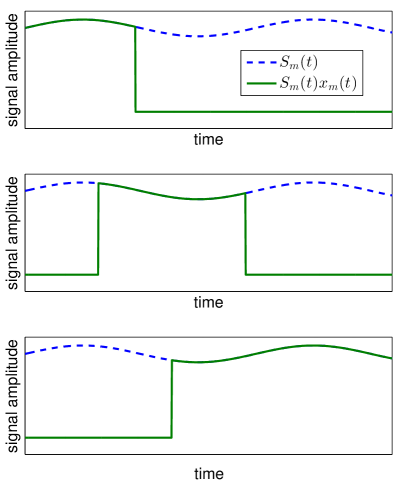
Figure 1: (Color online) Some example realizations of the signal component $S_{m}(t)x_{m}(t)$ of the observation process. Given a hypothesis $\mathcal{H}_{m}$, $S_{m}(t)$ is a deterministic signal amplitude and $x_{m}(t)$ is a binary stochastic process. The axes are in arbitrary units.

In stochastic detection theory, it is convenient to define a normalized observation process $y(t)$ as the time integral of $z(t)$:

$$y(t) \equiv\int_{0}^{t}d\tau\frac{z(\tau)}{\sqrt{R(\tau)}},$$ (7)

and represent it using a stochastic differential equation:

$$\mathcal{H}_{m}:\ dy(t) \equiv y(t+dt)-y(t)$$

$$=dt\sigma_{m}(t)x_{m}(t)+dW(t),$$ (8)

$$\sigma_{m}(t) \equiv\frac{S_{m}(t)}{\sqrt{R(t)}},$$ (9)

where $W(t)$ is the standard Wiener process with increment variance $dW^{2}(t)=dt$ and Itō calculus Gardiner (2010); Mao (2007) is assumed throughout this paper. The null hypothesis, in particular, is taken to be

$$\mathcal{H}_{0}:dy(t) =dW(t).$$ (10)

Fig. 2 depicts the observation model through a block diagram.

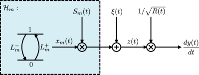
Figure 2: (Color online) A block diagram for the observation model. $\mathcal{H}_{m}$ is a hypothesis, $x_{m}(t)$ is the hidden signal, assumed here to be a two-state Markov process with transition rates $L_{m}^{-}$ and $L_{m}^{+}$, $S_{m}(t)$ is the signal amplitude, $\xi(t)$ is an additive white Gaussian noise, and $z(t)$ is the observation process. The definition of observation processes $dy(t)/dt$ and $y(t)$, normalized with respect to the noise power $R(t)$, is for mathematical convenience.

III.2 Estimator-correlator formula

Define the observation record as

$$Y^{T} \equiv\left\{y(t);0\leq t\leq T\right\}.$$ (11)

Under rather general conditions about $x_{m}(t)$, the LLR $\ln\Lambda(Y^{T}|\mathcal{H}_{m})$ can be expressed using the estimator-correlator formula Kailath and Poor (1998); Duncan (1968); Kailath (1969); Tsang (2012), which correlates the observation with an “assumptive” estimate $\mu_{m}(t)$:

$$\ln\Lambda(Y^{T}|\mathcal{H}_{m}) =\int_{0}^{T}dy(t)\mu_{m}(t)-\frac{1}{2}\int_{0}^{T}dt\mu_{m}^{2}(t),$$ (12)

where

$$\mu_{m}(t) \equiv\sigma_{m}(t)\operatorname{\mathbb{E}}\left[x_{m}(t)|Y^{t},\mathcal{H}_{m}\right]$$ (13)

is a causal estimator of the hidden signal conditioned on the observation record $Y^{t}$ and the hypothesis $\mathcal{H}_{m}$. The $dy(t)$ integral is an Itō integral, meaning that $dy(t)$ is the future increment ahead of time $t$ and $\mu_{m}(t)$ in the integrand $dy(t)\mu_{m}(t)$ should not depend on $dy(t)$. This rule is important for consistent analytic and numerical calculations whenever one multiplies $dy(t)$ with a signal that depends on $y(t)$ Kailath and Poor (1998). Fig. 3 illustrates an implementation of the formula.

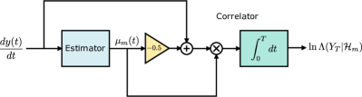
Figure 3: (Color online) An implementation of the estimator-correlator formula in Eq. (12), which can be written as $\ln\Lambda=\int_{0}^{T}[dy(t)-dt\mu_{m}(t)/2]\mu_{m}(t)$. $dy(t)$ in the integrand should be the future increment ahead of $t$ in accordance with Itō calculus.

As each $\ln\Lambda(Y^{T}|\mathcal{H}_{m})$ depends only on one hypothesis $\mathcal{H}_{m}$ (in addition to the fixed null hypothesis), once an algorithm for its computation is implemented, it can be re-used even if the other hypotheses are changed or new hypotheses are added. This makes the estimator-correlator protocol more flexible and extensible than the ones proposed in Refs. Gambetta et al. (2007); D’Anjou and Coish (2014), which are specific to the hypotheses considered there.

Despite its simple appearance, the formula does not in general reduce the complexity of the LLR calculation, as the estimator may still be difficult to implement. We shall, however, present a simple numerical method and some analytic solutions useful for the qubit readout problem in the following.

III.3 Qubit dynamics

For QND qubit readout, we assume that $x_{m}(t)$ is a classical two-state first-order Markov process; Appendix A shows explicitly how the classical theory can arise from the quantum formalism of continuous QND measurement. The possible values of $x_{m}(t)$ are assumed to be

$$x_{m}(t) \in\left\{0,1\right\}.$$ (14)

Other possibilities can be modeled by subtracting a baseline value from the actual observation and defining an appropriate $\sigma_{m}(t)$ before the processing described here. In the absence of measurements, the probability function of $x_{m}(t)=x$ obeys a forward Kolmogorov equation Gardiner (2010):

$$\frac{d\boldsymbol{P}_{m}(t)}{dt} =\boldsymbol{L}_{m}(t)\boldsymbol{P}_{m}(t),$$ (15)

$$\boldsymbol{P}_{m}(t) \equiv\left(\begin{array}[]{c}P(x=0,t|\mathcal{H}_{m})\\ P(x=1,t|\mathcal{H}_{m})\end{array}\right),$$ (18)

$$\boldsymbol{L}_{m}(t) \equiv\left(\begin{array}[]{cc}-L_{m}^{+}(t)&L_{m}^{-}(t)\\ L_{m}^{+}(t)&-L_{m}^{-}(t)\end{array}\right),$$ (21)

where $L_{m}^{-}$ and $L_{m}^{+}$ are the spontaneous decay and excitation rates conditioned on the hypothesis and can be time-varying for generality. The decay time constant $1/L_{m}^{-}$ is commonly called $T_{1}$, and $L_{m}^{+}$ can be used to model a random turn-on time D’Anjou and Coish (2014). For example, we can model the problem studied by Gambetta and coworkers Gambetta et al. (2007) by defining

• $\mathcal{H}_{0}$: the qubit is in the $x=0$ state, and $x_{0}(t)=0$.

• $\mathcal{H}_{1}$: the qubit is in the $x=1$ state initially, $P(x=1,t=0|\mathcal{H}_{1})=1$, and the unconditional statistics of $x_{1}(t)$ obey Eqs. (15)–(21), with $L_{1}^{-}$ being the decay rate and $L_{1}^{+}=0$.

III.4 Estimator

The estimator $\mu_{m}(t)$ can be computed using the Duncan-Mortensen-Zakai (DMZ) equation Duncan (1967); Mortensen (1966); Zakai (1969); Wong and Hajek (1985):

$$d\boldsymbol{p}_{m}(t) =dt\boldsymbol{L}_{m}(t)\boldsymbol{p}_{m}(t)+dy(t)\sigma_{m}(t)\boldsymbol{x}\boldsymbol{p}_{m}(t),$$ (22)

$$\boldsymbol{p}_{m}(t) \equiv\left(\begin{array}[]{c}p_{m}(x=0,t)\\ p_{m}(x=1,t)\end{array}\right),\quad\boldsymbol{x}\equiv\left(\begin{array}[]{cc}0&0\\ 0&1\end{array}\right),$$ (27)

where

$$p_{m}(x,t)\propto P(x,t|Y^{t},\mathcal{H}_{m})$$ (28)

is the unnormalized posterior probability function of $x_{m}(t)$ conditioned on $Y^{t}$ and $\mathcal{H}_{m}$, and the initial condition is determined by the initial prior probabilities:

$$p_{m}(x,t=0) =P(x,t=0|\mathcal{H}_{m}).$$ (29)

The estimator is then

$$\mu_{m}(t) =\frac{\sigma_{m}(t)p_{m}(1,t)}{p_{m}(0,t)+p_{m}(1,t)},$$ (30)

as depicted by Fig. 4.

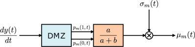
Figure 4: (Color online) A block diagram for the estimator using the Duncan-Mortensen-Zakai (DMZ) equation.

Although one can also use the Wonham equation Wonham (1964) to perform the estimator, and the normalization step would not be needed in theory, the DMZ equation is linear with respect to $\boldsymbol{p}_{m}(t)$ and easier to solve analytically or numerically. In general, a numerical split-step method can be used Higham et al. (2002):

$$\boldsymbol{p}_{m}(t+dt) \approx\exp\left[dy(t)\sigma_{m}(t)\boldsymbol{x}-\frac{dt}{2}\sigma_{m}^{2}(t)\boldsymbol{x}^{2}\right]$$

$$\quad\times\exp\left[dt\boldsymbol{L}_{m}(t)\right]\boldsymbol{p}_{m}(t).$$ (31)

Many other numerical methods are available Kloeden et al. (2003). Analytic solutions can be obtained in the following special cases.

III.5 Deterministic-signal detection

For a simple example, assume binary hypothesis testing ($M=2$), no spontaneous transition ($L_{m}^{-}=L_{m}^{+}=0$), and deterministic initial conditions given by

$$p_{0}(0,0)=P(x=0,t=0|\mathcal{H}_{0}) =1,$$ (32)

$$p_{0}(1,0)=P(x=1,t=0|\mathcal{H}_{0}) =0,$$ (33)

$$p_{1}(0,0)=P(x=0,t=0|\mathcal{H}_{1}) =0,$$ (34)

$$p_{1}(1,0)=P(x=1,t=0|\mathcal{H}_{1}) =1.$$ (35)

The estimator becomes independent of the observation:

$$\mu_{0}(t) =0, \mu_{1}(t) =\sigma_{1}(t).$$ (36)

This is simply a case of deterministic-signal detection, when the estimator-correlator formula in Eq. (12) becomes a matched filter Van Trees (2001); Kailath and Poor (1998). The minimum error probability $P_{e,\textrm{min}}$ has an analytic expression Van Trees (2001):

$$P_{e,\textrm{min}} =P_{+}P(\mathcal{H}_{0})+P_{-}P(\mathcal{H}_{1}),$$ (37)

$$P_{\pm} \equiv\frac{1}{2}\operatorname{erfc}\left[\sqrt{\frac{\textrm{SNR}}{8}}\left(1\pm\frac{2\lambda}{\textrm{SNR}}\right)\right],$$ (38)

$$\operatorname{erfc}u \equiv\frac{2}{\sqrt{\pi}}\int_{u}^{\infty}dv\exp(-v^{2}),$$ (39)

SNR $$\equiv\int_{0}^{T}dt\sigma_{1}^{2}(t),\quad\lambda\equiv\ln\frac{P(\mathcal{H}_{1})}{P(\mathcal{H}_{0})}.$$ (40)

For $\textrm{SNR}\to\infty$, the error exponent has the asymptotic behavior $-\ln P_{e,\textrm{min}}\to\textrm{SNR}/8$.

Although this solution for $P_{e,\textrm{min}}$ is not strictly valid when spontaneous transitions are present, it should be accurate when the observation time $T$ is short relative to $1/L_{1}^{-}$ or $1/L_{1}^{+}$ and can serve as a rough guide for other cases.

III.6 No spontaneous excitation ($L_{m}^{+}=0$)

The case of $L_{m}^{-}>0$ and $L_{m}^{+}=0$ corresponds to the model studied by Gambetta and coworkers Gambetta et al. (2007). Eq. (22) becomes

$$dp_{m}(0,t) =dtL_{m}^{-}(t)p_{m}(1,t),$$ (41)

$$dp_{m}(1,t) =-dtL_{m}^{-}(t)p_{m}(1,t)+dy(t)\sigma_{m}(t)p_{m}(1,t).$$ (42)

Eq. (42) describes the famous geometric Brownian motion Mao (2007). Its well known solution can be obtained by applying Itō’s lemma to $d\ln p_{m}(1,t)$ and is given by

$$p_{m}(1,t) =p_{m}(1,0)\exp\left\{\int_{0}^{t}dy(\tau)\sigma_{m}(\tau)\right.$$

$$\quad\left.-\int_{0}^{t}d\tau\left[\frac{\sigma_{m}^{2}(\tau)}{2}+L_{m}^{-}(\tau)\right]\right\}.$$ (43)

A time integral of $p_{m}(1,t)$ then gives $p_{m}(0,t)$:

$$p_{m}(0,t) =p_{m}(0,0)+\int_{0}^{t}d\tau L_{m}^{-}(\tau)p_{m}(1,\tau).$$ (44)

For binary qubit state discrimination, we can assume that $\mu_{0}(t)=0$, and $\mu_{1}(t)$ can be determined from Eqs. (43), (44), and (30), starting from the deterministic initial conditions given by Eqs. (34) and (35) if the measurement starts immediately after the qubit state is prepared, as shown in Fig. 5. If there is a finite arming time before the measurement starts Gambetta et al. (2007); D’Anjou and Coish (2014), the forward Kolmogorov equation (15) can be used to determine the initial state probabilities.

Figure 5: (Color online) Solution to the DMZ equation with spontaneous decay ($L_{m}^{-}>0$), no spontaneous excitation ($L_{m}^{+}=0$), and an initial excited state ($p_{m}(1,t=0)=1$, $p_{m}(0,t=0)=0$).

III.7 No spontaneous decay ($L_{m}^{-}=0$)

One can assume $L_{m}^{+}>0$ and $L_{m}^{-}=0$ to model a random signal turn-on time D’Anjou and Coish (2014) and negligible spontaneous decay ($T\ll 1/L_{m}^{-}$). The simplest way of computing $\mu_{m}(t)$ is to define a new observation process

$$dy^{\prime}(t) \equiv dy(t)-\sigma_{m}(t)dt$$

$$=-dt\sigma_{m}(t)\left[1-x_{m}(t)\right]+dW(t).$$ (45)

A new DMZ equation can then be expressed in terms of $y^{\prime}(t)$ and is given by

$$dp_{m}(0,t) =-dtL_{m}^{+}(t)p_{m}(0,t)-dy^{\prime}(t)\sigma_{m}(t)p_{m}(0,t),$$ (46)

$$dp_{m}(1,t) =dtL_{m}^{+}(t)p_{m}(0,t),$$ (47)

which have the same form as Eqs. (41) and (42) and can be solved using the same method. The final solution is

$$p_{m}(0,t) =p_{m}(0,0)\exp\left\{-\int_{0}^{t}dy(\tau)\sigma_{m}(\tau)\right.$$

$$\quad\left.+\int_{0}^{t}d\tau\left[\frac{\sigma_{m}^{2}(\tau)}{2}-L_{m}^{+}(\tau)\right]\right\},$$ (48)

$$p_{m}(1,t) =p_{m}(1,0)+\int_{0}^{t}d\tau L_{m}^{+}(\tau)p_{m}(0,\tau).$$ (49)

IV Poissonian noise model

IV.1 Observation process

For photon-counting measurements, it is more appropriate to assume that the counting process $n(t)\in\{0,1,2,\dots\}$, conditioned on the hidden process $X_{m}^{t}\equiv\{x_{m}(\tau);0\leq\tau\leq t\}$, obeys Poissonian statistics Snyder and Miller (1991):

$$\quad P(n(t)|X_{m}^{t},\mathcal{H}_{m})$$

$$=\exp\left[-\int_{0}^{t}d\tau\lambda_{m}(\tau)\right]\frac{\left[\int_{0}^{t}d\tau\lambda_{m}(\tau)\right]^{n(t)}}{n(t)!},$$ (50)

where

$$\lambda_{m}(t) \equiv\lambda_{0}(t)\left[1+\alpha_{m}(t)x_{m}(t)\right]$$ (51)

is the intensity of the Poisson process and $\alpha_{m}(t)$ is a deterministic signal amplitude. $dn(t)\in\{0,1\}$ is then the detected photon number at time $t$. We assume $\mathcal{H}_{0}$ with known intensity $\lambda_{0}(t)>0$ to be the null hypothesis.

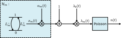
Figure 6: (Color online) The Poissonian observation model. The counting process $n(t)$ is driven by the stochastic intensity $\lambda_{m}(t)$.

IV.2 Estimator-correlator formula

Define the observation record as

$$N^{T} \equiv\left\{n(t);t_{0}\leq t\leq T\right\}.$$ (52)

Our goal is to calculate the LLR

$$\ln\Lambda(N^{T}|\mathcal{H}_{m}) =\ln\frac{dP(N^{T}|\mathcal{H}_{m})}{dP(N^{T}|\mathcal{H}_{0})}.$$ (53)

A formula analogous to the Gaussian case in Eq. (12) is given by Snyder (1972); Tsang (2012)

$$\ln\Lambda(N^{T}|\mathcal{H}_{m}) =\int_{0}^{T}dn(t)\ln\left[1+\nu_{m}(t)\right]$$

$$\quad-\int_{0}^{T}dt\lambda_{0}(t)\nu_{m}(t),$$ (54)

$$\nu_{m}(t) \equiv\alpha_{m}(t)\operatorname{\mathbb{E}}\left[x_{m}(t)|N^{t},\mathcal{H}_{m}\right],$$ (55)

where the $dn(t)$ integral should again follow Itō’s convention Snyder and Miller (1991). Fig. 7 illustrates the formula.

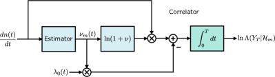
Figure 7: (Color online) The estimator-correlator structure for the Poissonian observation model. $dn(t)$ should be the future increment ahead of $t$ when multiplied with $\ln[1+\nu_{m}(t)]$.

IV.3 Estimator

We assume the same unconditional qubit dynamics described in Sec. III.3. The estimator can be computed from a DMZ-type equation Wong and Hajek (1985); Tsang (2012):

$$d\boldsymbol{p}_{m}(t) =dt\boldsymbol{L}_{m}(t)\boldsymbol{p}_{m}(t)+\left[dn(t)-dt\kappa(t)\right]$$

$$\quad\times\left\{\frac{\lambda_{0}(t)}{\kappa(t)}\left[\boldsymbol{I}+\alpha_{m}(t)\boldsymbol{x}\right]-\boldsymbol{I}\right\}\boldsymbol{p}_{m}(t),$$ (56)

where $\kappa(t)>0$ is an arbitrary positive reference intensity and the estimator is

$$\nu_{m}(t) =\frac{\alpha_{m}(t)p_{m}(1,t)}{p_{m}(0,t)+p_{m}(1,t)}.$$ (57)

This procedure is identical to that depicted in Fig. 4. Assuming $\kappa(t)=\lambda_{0}(t)$, Eq. (56) can be solved using a numerical split-step method:

$$\quad\boldsymbol{p}_{m}(t+dt)$$

$$\approx\exp\left\{dn(t)\ln\left[\boldsymbol{I}+\alpha_{m}(t)\boldsymbol{x}\right]-dt\lambda_{0}(t)\alpha_{m}(t)\boldsymbol{x}\right\}$$

$$\quad\times\exp\left[dt\boldsymbol{L}_{m}(t)\right]\boldsymbol{p}_{m}(t).$$ (58)

Analytic solutions can be found in the following cases.

IV.4 No spontaneous excitation ($L_{m}^{+}=0$)

Let $\kappa(t)=\lambda_{0}(t)$. Eq. (56) becomes

$$dp_{m}(0,t) =dtL_{m}^{-}(t)p_{m}(1,t),$$ (59)

$$dp_{m}(1,t) =-dtL_{m}^{-}(t)p_{m}(1,t)$$

$$\quad+\left[dn(t)-dt\lambda_{0}(t)\right]\alpha_{m}(t)p_{m}(1,t).$$ (60)

Following Chap. 5.3.1 in Ref. Snyder and Miller (1991), we get

$$p_{m}(1,t) =p_{m}(1,0)\exp\left\{\int_{0}^{t}dn(\tau)\ln\left[1+\alpha_{m}(\tau)\right]\right.$$

$$\quad\left.-\int_{0}^{t}d\tau\left[\lambda_{0}(\tau)\alpha_{m}(\tau)+L_{m}^{-}(\tau)\right]\right\},$$ (61)

$$p_{m}(0,t) =p_{m}(0,0)+\int_{0}^{t}d\tau L_{m}^{-}(\tau)p_{m}(1,\tau).$$ (62)

Fig. 8 depicts a block diagram for this solution.

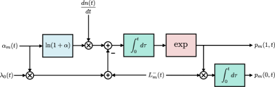
Figure 8: (Color online) A block diagram for Eqs. (61) and (62), a solution to the Poissonian DMZ equation. $L_{m}^{+}=0$, $p_{m}(1,t=0)=1$, and $p_{m}(0,t=0)=0$ are assumed.

IV.5 No spontaneous decay ($L_{m}^{-}=0$)

We now let $\kappa(t)=\lambda_{0}(t)\left[1+\alpha_{m}(t)\right]$. Eq. (56) becomes

$$dp_{m}(0,t) =-dtL_{m}^{+}(t)p_{m}(0,t)$$

$$\quad-\left[dn(t)-dt\kappa(t)\right]\frac{\alpha_{m}(t)}{1+\alpha_{m}(t)}p_{m}(0,t),$$ (63)

$$dp_{m}(1,t) =dtL_{m}^{+}(t)p_{m}(0,t).$$ (64)

Similar to the previous case, the solution is

$$p_{m}(0,t) =p_{m}(0,0)\exp\left\{-\int_{0}^{t}dn(\tau)\ln\left[1+\alpha_{m}(\tau)\right]\right.$$

$$\quad+\left.\int_{0}^{t}d\tau\left[\lambda_{0}(\tau)\alpha_{m}(\tau)-L_{m}^{+}(\tau)\right]\right\},$$ (65)

$$p_{m}(1,t) =p_{m}(1,0)+\int_{0}^{t}d\tau L_{m}^{+}(\tau)p_{m}(0,\tau).$$ (66)

It is interesting to note that all the Poissonian results approach the Gaussian ones in Sec. III if we assume $dn=\sqrt{\lambda_{0}}dy+\lambda_{0}dt$, $\alpha_{m}=\sigma_{m}/\sqrt{\lambda_{0}}$, and $\lambda_{0}\to\infty$.

V Conclusion

We have proposed an estimator-correlator architecture for optimal qubit-readout signal processing and found analytic solutions in some special cases of interest using Itō calculus. Although we have focused on a classical model, our formalism can potentially be extended to more general quantum dynamics Tsang (2012); Cook et al. (2014) and more realistic measurements, including artifacts such as dark counts and finite detector bandwidth Wiseman and Milburn (2010). An open problem of interest is the evaluation of readout performance beyond the case of deterministic-signal detection. Numerical Monte Carlo simulation is not difficult for two-level systems, but analytic solutions should bring additional insight and may be possible using tools in classical and quantum detection theory Van Trees (2001); Bucklew (1990); Helstrom (1976); Tsang and Nair (2012); Tsang (2014, 2013). Another open problem is the accuracy, speed, and practicality of our algorithms in reality, which will be subject to more specific experimental requirements and hardware limitations Stockton et al. (2002).

Appendix A Quantum formalism of continuous quantum-nondemolition measurement

Let

$$\hat{f}_{m}(t) =\left(\begin{array}[]{cc}f_{m}(0,0,t)&f_{m}(0,1,t)\\ f_{m}(1,0,t)&f_{m}(1,1,t)\end{array}\right)$$ (69)

be the unnormalized density matrix for the qubit conditioned on the observation record $Y^{t}$ and hypothesis $\mathcal{H}_{m}$. Consider the following linear stochastic quantum master equation Wiseman and Milburn (2010):

$$d\hat{f}_{m} =dtL_{m}^{-}\left(\hat{\sigma}_{-}\hat{f}_{m}\hat{\sigma}_{+}-\frac{1}{2}\hat{\sigma}_{+}\hat{\sigma}_{-}\hat{f}_{m}-\frac{1}{2}\hat{f}_{m}\hat{\sigma}_{+}\hat{\sigma}_{-}\right)$$

$$\quad+dtL_{m}^{+}\left(\hat{\sigma}_{+}\hat{f}_{m}\hat{\sigma}_{-}-\frac{1}{2}\hat{\sigma}_{-}\hat{\sigma}_{+}\hat{f}_{m}-\frac{1}{2}\hat{f}_{m}\hat{\sigma}_{-}\hat{\sigma}_{+}\right)$$

$$\quad+dtL_{m}^{x}\left(\hat{x}\hat{f}_{m}\hat{x}-\frac{1}{2}\hat{x}^{2}\hat{f}_{m}-\frac{1}{2}\hat{f}_{m}\hat{x}^{2}\right)$$

$$\quad+\frac{dy\sigma_{m}}{2}\left(\hat{x}\hat{f}_{m}+\hat{f}_{m}\hat{x}\right),$$ (70)

where

$$\hat{\sigma}_{-} =\left(\begin{array}[]{cc}0&1\\ 0&0\end{array}\right), \hat{\sigma}_{+} =\left(\begin{array}[]{cc}0&0\\ 1&0\end{array}\right), \hat{x} =\left(\begin{array}[]{cc}0&0\\ 0&1\end{array}\right),$$ (77)

and $L_{m}^{-}$, $L_{m}^{+}$, and $L_{m}^{x}\geq\sigma_{m}^{2}/4$ are the decay, excitation, and dephasing rates, respectively. The estimator in the quantum estimator-correlator formula Tsang (2012) is

$$\sigma_{m}(t)\operatorname{\mathbb{E}}\left(\hat{x}|Y^{t},\mathcal{H}_{m}\right) =\frac{\sigma_{m}(t)f_{m}(1,1,t)}{f_{m}(0,0,t)+f_{m}(1,1,t)}.$$ (78)

The important point here is that the estimator involves only the diagonal components of $\hat{f}_{m}(t)$, which are decoupled from the off-diagonal components throughout the evolution:

$$df_{m}(0,0,t) =dt\left[-L_{m}^{+}(t)f_{m}(0,0,t)+L_{m}^{-}(t)f_{m}(1,1,t)\right],$$ (79)

$$df_{m}(1,1,t) =dt\left[L_{m}^{+}(t)f_{m}(0,0,t)-L_{m}^{-}(t)f_{m}(1,1,t)\right]$$

$$\quad+dy(t)\sigma_{m}(t)f_{m}(1,1,t).$$ (80)

This means that a classical stochastic model is sufficient. In particular, Eqs. (79) and (80) are identical to the classical DMZ equation given by Eq. (22). The argument in the case of Poissonian noise is similar.

References

- Wiseman and Milburn (2010) H. M. Wiseman and G. J. Milburn, Quantum Measurement and Control (Cambridge University Press, Cambridge, 2010).
- Wallraff et al. (2005) A. Wallraff, D. I. Schuster, A. Blais, L. Frunzio, J. Majer, M. H. Devoret, S. M. Girvin, and R. J. Schoelkopf, Phys. Rev. Lett. 95, 060501 (2005).
- Lupascu et al. (2007) A. Lupascu, S. Saito, T. Picot, P. C. de Groot, C. J. P. M. Harmans, and J. E. Mooij, Nature Physics 3, 119 (2007).
- Johnson et al. (2012) J. E. Johnson, C. Macklin, D. H. Slichter, R. Vijay, E. B. Weingarten, J. Clarke, and I. Siddiqi, Phys. Rev. Lett. 109, 050506 (2012).
- Hume et al. (2007) D. B. Hume, T. Rosenband, and D. J. Wineland, Phys. Rev. Lett. 99, 120502 (2007).
- Myerson et al. (2008) A. H. Myerson, D. J. Szwer, S. C. Webster, D. T. C. Allcock, M. J. Curtis, G. Imreh, J. A. Sherman, D. N. Stacey, A. M. Steane, and D. M. Lucas, Phys. Rev. Lett. 100, 200502 (2008).
- Neumann et al. (2010) P. Neumann, J. Beck, M. Steiner, F. Rempp, H. Fedder, P. R. Hemmer, J. Wrachtrup, and F. Jelezko, Science 329, 542 (2010).
- Robledo et al. (2011) L. Robledo, L. Childress, H. Bernien, B. Hensen, P. F. A. Alkemade, and R. Hanson, Nature 477, 574 (2011).
- Elzerman et al. (2004) J. M. Elzerman, R. Hanson, L. H. Willems van Beveren, B. Witkamp, L. M. K. Vandersypen, and L. P. Kouwenhoven, Nature 430, 431 (2004).
- Vamivakas et al. (2010) A. N. Vamivakas, C.-Y. Lu, C. Matthiesen, Y. Zhao, S. Falt, A. Badolato, and M. Atature, Nature 467, 297 (2010).
- Morello et al. (2010) A. Morello, J. J. Pla, F. A. Zwanenburg, K. W. Chan, K. Y. Tan, H. Huebl, M. Mottonen, C. D. Nugroho, C. Yang, J. A. van Donkelaar, A. D. C. Alves, D. N. Jamieson, C. C. Escott, L. C. L. Hollenberg, R. G. Clark, and A. S. Dzurak, Nature 467, 687 (2010).
- Pla et al. (2013) J. J. Pla, K. Y. Tan, J. P. Dehollain, W. H. Lim, J. J. L. Morton, F. A. Zwanenburg, D. N. Jamieson, A. S. Dzurak, and A. Morello, Nature 496, 334 (2013).
- Nielsen and Chuang (2011) M. A. Nielsen and I. L. Chuang, Quantum Computation and Quantum Information (Cambridge University Press, Cambridge, 2011).
- Rondin et al. (2014) L. Rondin, J.-P. Tetienne, T. Hingantm, J.-F. Roch, P. Maletinsky, and V. Jacques, Reports on Progress in Physics 77, 056503 (2014).
- Schmidt et al. (2005) P. O. Schmidt, T. Rosenband, C. Langer, W. M. Itano, J. C. Bergquist, and D. J. Wineland, Science 309, 749 (2005).
- Chou et al. (2010) C. W. Chou, D. B. Hume, T. Rosenband, and D. J. Wineland, Science 329, 1630 (2010).
- Gambetta et al. (2007) J. Gambetta, W. A. Braff, A. Wallraff, S. M. Girvin, and R. J. Schoelkopf, Phys. Rev. A 76, 012325 (2007).
- D’Anjou and Coish (2014) B. D’Anjou and W. A. Coish, Phys. Rev. A 89, 012313 (2014).
- Van Trees (2001) H. L. Van Trees, Detection, Estimation, and Modulation Theory, Part I. (John Wiley & Sons, New York, 2001).
- Kailath and Poor (1998) T. Kailath and H. V. Poor, IEEE Transactions on Information Theory 44, 2230 (1998).
- Duncan (1968) T. E. Duncan, Information and Control 13, 62 (1968).
- Kailath (1969) T. Kailath, IEEE Transactions on Information Theory 15, 350 (1969).
- Snyder (1972) D. L. Snyder, IEEE Transactions on Information Theory 18, 91 (1972).
- Braginsky and Khalili (1992) V. B. Braginsky and F. Y. Khalili, Quantum Measurement (Cambridge University Press, Cambridge, 1992).
- Tsang and Caves (2012) M. Tsang and C. M. Caves, Phys. Rev. X 2, 031016 (2012).
- Gough and James (2009) J. Gough and M. James, IEEE Transactions on Automatic Control 54, 2530 (2009).
- Snyder and Miller (1991) D. L. Snyder and M. I. Miller, Random Point Processes in Time and Space (Springer-Verlag, New York, 1991).
- Tsang (2012) M. Tsang, Phys. Rev. Lett. 108, 170502 (2012).
- Stockton et al. (2002) J. Stockton, M. Armen, and H. Mabuchi, J. Opt. Soc. Am. B 19, 3019 (2002).
- Gardiner (2010) C. W. Gardiner, Stochastic Methods: A Handbook for the Natural and Social Sciences (Springer, Berlin, 2010).
- Mao (2007) X. Mao, Stochastic Differential Equations and Applications (Woodhead, Oxford, 2007).
- Gambetta and Wiseman (2001) J. Gambetta and H. M. Wiseman, Phys. Rev. A 64, 042105 (2001).
- Chase and Geremia (2009) B. A. Chase and J. M. Geremia, Phys. Rev. A 79, 022314 (2009).
- Blume-Kohout et al. (2010) R. Blume-Kohout, J. O. S. Yin, and S. J. van Enk, Phys. Rev. Lett. 105, 170501 (2010).
- Wiebe et al. (2014) N. Wiebe, C. Granade, C. Ferrie, and D. Cory, Phys. Rev. A 89, 042314 (2014).
- Combes et al. (2014) J. Combes, C. Ferrie, C. Cesare, M. Tiersch, G. J. Milburn, H. J. Briegel, and C. M. Caves, ArXiv e-prints (2014), arXiv:1405.5656 [quant-ph] .
- Berger (1985) J. O. Berger, Statistical Decision Theory and Bayesian Analysis (Springer-Verlag, New York, 1985).
- Duncan (1967) T. E. Duncan, Probability densities for diffusion processes with applications to nonlinear filtering theory and detection theory, Ph.D. thesis, Stanford University (1967).
- Mortensen (1966) R. E. Mortensen, Optimal control of continuous-time stochastic systems, Ph.D. thesis, University of California, Berkeley (1966).
- Zakai (1969) M. Zakai, Zeitschrift für Wahrscheinlichkeitstheorie und Verwandte Gebiete 11, 230 (1969).
- Wong and Hajek (1985) E. Wong and B. Hajek, Stochastic Processes in Engineering Systems (Springer-Verlag, New York, 1985).
- Wonham (1964) W. Wonham, Journal of the Society for Industrial and Applied Mathematics Series A Control 2, 347 (1964).
- Higham et al. (2002) D. J. Higham, X. Mao, and A. M. Stuart, SIAM Journal on Numerical Analysis 40, 1041 (2002).
- Kloeden et al. (2003) P. E. Kloeden, E. Platen, and H. Schurz, Numerical Solution of SDE Through Computer Experiments (Springer, Berlin, 2003).
- Cook et al. (2014) R. L. Cook, C. A. Riofrío, and I. H. Deutsch, ArXiv e-prints (2014), arXiv:1406.4482 [quant-ph] .
- Bucklew (1990) J. A. Bucklew, Large Deviation Techniques in Decision, Simulation, and Estimation (Wiley, New York, 1990).
- Helstrom (1976) C. W. Helstrom, Quantum Detection and Estimation Theory (Academic Press, New York, 1976).
- Tsang and Nair (2012) M. Tsang and R. Nair, Phys. Rev. A 86, 042115 (2012).
- Tsang (2014) M. Tsang, ArXiv e-prints (2014), arXiv:1310.0291 [quant-ph] .
- Tsang (2013) M. Tsang, Quantum Measurements and Quantum Metrology 1, 84 (2013).