Pinning time statistics for vortex lines in disordered environments

Abstract

We study the pinning dynamics of magnetic flux (vortex) lines in a disordered type-II superconductor. Using numerical simulations of a directed elastic line model, we extract the pinning time distributions of vortex line segments. We compare different model implementations for the disorder in the surrounding medium: discrete, localized pinning potential wells that are either attractive and repulsive or purely attractive, and whose strengths are drawn from a Gaussian distribution; as well as continuous Gaussian random potential landscapes. We find that both schemes yield power law distributions in the pinned phase as predicted by extreme-event statistics, yet they differ significantly in their effective scaling exponents and their short-time behavior.

I Introduction

The static and dynamic properties of elastic manifolds in random media have been central research topics of statistical physics for decades (see, e.g., Refs. Fisher1998 ; Brazovskii2004 ). Specifically, fluctuating directed lines interacting with spatially uncorrelated disorder represent the basic model for magnetic vortices in type-II superconductors with point pinning centers Blatter1994 , crystal dislocations Ioffe1987 , as well as for aligned polymers Ertas1992 ; Ertas1996 ; Kardar1998 . There are also fascinating intimate mathematical connections with the dynamics of driven interfaces and non-equilibrium growth processes HalpinHealy1995 ; Rosso2003 . A system of directed lines, subject to competing thermal fluctuations and pinning from a random disorder background, constitutes a remarkably complex system displaying a rich thermodynamic phase diagram and a wealth of distinct dynamical regimes Blatter1994 ; Agoritsas2012 , as well as intriguing non-equilibrium relaxation kinetics Du2007 ; Pleimling2011 ; Dobramysl2013 ; Assi2014 . In particular, driven elastic strings in a random medium show a transition between a pinned vortex glass phase, in which the dynamics are dominated by thermally activated creep, and a flowing phase above a critical depinning force Nattermann2000 . Both phases possess rich dynamical features Duemmer2005 ; Kolton2009 , with universal depinning force distributions Bolech2004 and scaling behavior Bustingorry2010 at the critical point.

In this work, we focus on the statistical distribution of dwelling times of line segments localized at the defects, which incorporates information on the collective Larkin–Ovchinnikov pinning scale. We perform detailed computer simulations to investigate how distinct model representations of the disordered environment affect the depinning kinetics, and compare our numerical data with the hitherto unconfirmed theoretical predictions of Ref. Vinokur1996 . We begin by introducing our model Hamiltonian and providing key theoretical background. We then describe our dynamical simulation method based on an overdamped Langevin equation. We next discuss different disorder implementations, our simulation protocol, and the measurement procedures we employ in order to extract pinning time distributions. We then proceed with a brief analysis of the effects of overlapping disorder potentials, and the transition between the pinned and free-flowing phases. Our principal results concern the dwelling time statistics from simulations with either discrete, localized pinning potential wells, or with smooth Gaussian pinning landscapes.

II Theoretical Background

We consider non-interacting (independent) vortex lines driven through a three-dimensional disordered superconductor, with the orienting magnetic field aligned with the $z$ direction. Line segments can move in the perpendicular $xy$ plane, but cannot form loops. The corresponding coarse-grained Hamiltonian for the directed lines is given by Nelson1993 ; Blatter1994

$$\mathcal{H}[\vec{r}]=\int_{0}^{\gamma L}\biggl{[}\frac{\epsilon}{2}\biggl{|}\frac{d\vec{r}(z)}{dz}\biggr{|}^{2}+U\bigl{(}\vec{r}(z),z\bigr{)}\biggr{]}dz\ .$$ (1)

It constitutes the effective energy functional of the two-dimensional vector $\vec{r}(z)$ that defines the line position along the line axis $z$, i.e. the line trajectory at a given time. The requirement that the directed elastic lines may not form loops is reflected in the condition that $\vec{r}(z)$ be surjective. The line tension $\epsilon$ is the elastic energy per unit length, and $U\bigl{(}\vec{r}(z),z\bigr{)}$ represents the disorder potential. Its detailed implementation for either discrete pinning sites or a smooth potential landscape will be described below. To suppress surface effects, we employ periodic conditions along the $z$ direction (identifying $z=\gamma L$ with $z=0$).

In order to capture the dynamics of our vortex system, we employ overdamped Langevin dynamics Brass1989 ; Dobramysl2013 :

$$\eta\,\frac{\partial\vec{r}(z,t)}{\partial t}=-\frac{\delta\mathcal{H}[\vec{r}]}{\delta\vec{r}(z,t)}+\vec{f}(z,t)+\vec{F}\ .$$ (2)

Here, $\eta$ is the viscosity of the surrounding medium. For magnetic flux lines, it is given by the Bardeen–Stephen viscous drag parameter Bardeen1965 . The constant force density vector $\vec{F}$ represents the external drive. Fast, microscopic degrees of freedom stemming from interactions with the surrounding medium are captured via thermal stochastic forcing, modeled as uncorrelated Gaussian white noise with zero mean $\langle\vec{f}(z,t)\rangle=0$ and the second moment $\langle f_{\alpha}(z,t)f_{\beta}(z^{\prime},t^{\prime})\rangle=2\eta T\delta_{\alpha\beta}\,\delta(z-z^{\prime})\delta(t-t^{\prime})$ ($\alpha,\beta=x,y$), satisfying Einstein’s relation for thermal equilibrium at temperature $T$ (we set Boltzmann’s constant $k_{\rm B}=1$).

The vortices are thus subject to various energy scales: (i) the internal elastic energy, (ii) the (random) disorder potential, (iii) an external driving force, and (iv) thermal fluctuations stemming from interactions with the surrounding medium. Varying the strengths of these competing contributions leads to remarkably rich and complex dynamics. At $T=0$, there exists a sharp continuous transition at a critical driving force $F_{c}$ separating a pinned vortex phase from a non-equilibrium steady state in which the lines are freely flowing Blatter1994 ; Vinokur1996 ; Fisher1998 . At finite temperatures, the dynamic phase transition is thermally rounded, resulting in line motion (flux creep) even below the critical depinning force Fisher1998 . Depending on the spatial distribution and strength of the disorder, the transverse line roughness displays intriguing behavior near $F_{c}$ Dobramysl2013 .

The relevant length scale in the pinned phase is given by the Larkin–Ovchinnikov pinning length $L_{L}=\xi(\epsilon/w)^{2/3}$, with $\xi$ and $w$ denoting the spatial range of disorder correlations and the standard deviation of the disorder potential strength. $L_{L}$ measures the typical extent of collectively pinned line segments Vinokur1996 . The transition to the free-flowing phase occurs when the driving force becomes large enough to cause displacements on the order of $L_{L}$. Associated with this length scale is a minimum energy barrier between pinned configurations $E_{L}\approx\epsilon\xi^{2}/L_{L}$. Thus one may estimate the critical force (per line element length) as $F_{c}\approx E_{L}/(\xi L_{L})\approx w^{4/3}/(\xi\epsilon^{1/3})$. Using arguments based on extreme-event statistics, Vinokur, Marchetti and Chen found that the pinning time distribution of line segments should obey a power law for large dwell times $\tau$,

$$P(\tau)\propto\tau^{-1-\alpha}\ ,\quad\alpha\propto T/E_{L}\ ,$$ (3)

with a scaling exponent $\alpha<1$ for low temperatures Vinokur1996 . In their derivation, Vinokur et al. assumed a Gaussian-distributed disorder potential with a spatial correlation length $\xi$. However, material defects in superconducting samples should more realistically be represented by discrete and moreover purely attractive pinning sites instead of a continuous disordered landscape with zero mean. We remark that studies of non-equilibrium vortex relaxation kinetics have emphasized the drastic influence of the underlying pinning model Iguain2009 ; Pleimling2011 . At any rate, the intriguing theoretical prediction (3) has not yet been numerically tested (nor experimentally confirmed).

III Model Description

III.1 Discretized elastic line model

In order to facilitate computational modeling of this system, we discretize the elastic line into connected nodes with a spacing $\gamma$ along the $z$ axis. Line tension is implemented via an elastic interaction between adjacent nodes. The ensuing discretized Hamiltonian reads

$$H(\{\vec{r}_{k}\})=\sum_{k=1}^{L}\biggl{[}\frac{\epsilon}{4\gamma}|\vec{r}_{k-1}+\vec{r}_{k+1}-2\vec{r}_{k}|^{2}+\gamma U(\vec{r}_{k},k\gamma)\biggr{]}\ ,$$ (4)

where $k=0$ maps to $k=L$ in order to correctly account for the periodic boundaries in the $z$ direction. We now have to numerically solve the coupled Langevin equations

$$\gamma\eta\,\frac{\partial\vec{r}_{j}(t)}{\partial t}=-\frac{\partial H(\{\vec{r}_{k}\})}{\partial\vec{r}_{j}(t)}+\vec{f}_{j}(t)+\gamma\vec{F}$$ (5)

with $\vec{f}_{j}(t)=\gamma\vec{f}(z,t)$; following Ref. Brass1989 , we perform the temporal integration via the Euler–Maruyama method.

In the following, all lengths are measured in terms of the pinning center radius $b_{0}=3.5\,\text{nm}$, and energies relative to the intrinsic vortex line energy $\epsilon_{0}b_{0}$. Inserting parameter values that correspond to the high-$T_{c}$ superconducting compound YBCO, one obtains $\epsilon_{0}\approx 1.92\times 10^{-6}\,\text{erg}/\text{cm}$ Pleimling2011 . The vortex line tension in this anisotropic material is $\epsilon\approx 0.189\epsilon_{0}$, whence the Bardeen–Stephen viscous drag coefficient becomes $\eta\approx 10^{-10}\text{erg}\times\text{s}/\text{cm}^{3}$, which yields the fundamental simulation time unit $t_{0}\approx 18\,\text{ps}$ Dobramysl2013 . We set the layer spacing equal to the pinning center radius $\gamma=b_{0}$. In previous work Dobramysl2013 ; Assi2014 , we have extensively tested this discretized elastic line model, and verified that it correctly reproduces the expected thermodynamic phases (for $\vec{F}=0$) as well as the established non-equilibrium steady-state properties at finite drive current.

III.2 Disorder potential

We investigate and compare fundamentally different disorder implementations: discrete potential wells with varying strengths, and Gaussian distributed potential landscapes with a finite correlation length. The former scheme constitutes a more realistic model of localized pinning sites for flux lines in type-II superconductors Pleimling2011 ; Dobramysl2013 , while the latter is specifically amenable to analytic investigations such as Ref. Vinokur1996 .

III.2.1 Discrete pinning sites

In type-II superconductors, material defects such as oxygen vacancies take the form of randomly distributed discrete potential wells. They act as short-ranged pinning centers wherein magnetic flux lines may be trapped. (In this work, we only consider uncorrelated point-like disorder.) We model these individual pinning sites as an ensemble of $N_{k}$ smooth, radially symmetric potential wells per layer $k$, centered at ${\vec{r}}^{\,(i)}_{k}$:

$$U(\vec{r}_{k},k\gamma)=\sum_{i=1}^{N_{k}}\frac{p^{(i)}_{k}}{2}\Bigl{(}1-\tanh\Bigl{[}5\bigl{(}\big{|}\vec{r}_{k}-\vec{r}^{\,(i)}_{k}\big{|}/b_{0}-1\bigr{)}\Bigr{]}\Bigr{)}\ .$$ (6)

The pinning potential strengths $p^{(i)}_{k}$ are Gaussian random variables with mean $\big{\langle}p^{(i)}_{k}\big{\rangle}=\mu$ and variance $\big{\langle}p^{(i)}_{k}p^{(j)}_{l}\big{\rangle}=w^{2}\delta_{ij}\delta_{kl}$. The pin positions $\vec{r}^{\,(i)}_{k}$ ($i=1,\ldots,N_{k}$) are uniformly distributed throughout the $xy$ domain, independently in each layer $k$. Overlaps between pinning sites are avoided, hence the minimal distance between sites is $\big{|}\vec{r}^{\,(i)}_{k}-\vec{r}^{\,(j)}_{l}\big{|}>2b_{0}$. (The effects of overlapping defect potentials in the depinned phase will be discussed below.)

III.2.2 Continuous disorder landscape

Alternatively, we employ a Gaussian pinning potential landscape in order to connect to the model considered by Vinokur et al. Vinokur1996 . To generate a continuous smooth disorder landscape, we draw a potential value from a Gaussian distribution at each node of a square lattice with spacing $\xi$. Such a lattice is constructed independently for each layer $k$. The value of the disorder potential at an arbitrary point $(\vec{r}_{k},k\gamma)$ is then determined via a bilinear interpolation of the values defined on the lattice nodes. The potential landscape $U(\vec{r},z)$ resulting from this procedure is characterized by correlations on the order of the lattice spacing $\xi$: $\big{\langle}U(\vec{r},k\gamma)U(\vec{r\,}^{\prime},l\gamma)\big{\rangle}=w^{2}\delta_{kl}f\bigl{(}|\vec{r}-\vec{r\,}^{\prime}|/\xi\bigr{)}$ with a (roughly exponentially) decaying function $f$, similar to Ref. Vinokur1996 . In comparisons with discrete localized pinning potentials, we set $\xi=b_{0}$.

IV Simulation procedure

IV.1 Initialization

We initialize a simulation by creating a computational domain of length $l=100b_{0}$ (along the direction of the driving force), width $W=10b_{0}$, and height $\gamma L$, with $L=200$ and periodic boundary conditions in all directions. We have systematically varied the line length and found no finite-size effects already at this value of $L$. Depending on the desired type of disorder, we either randomly distribute discrete pinning centers throughout the domain, or create a continuous disorder landscape through interpolation from normal-distributed lattice potential values. The resulting force field is then used in the numerical solution of Eqs. (5).

Ten lines are then introduced at regular intervals along the system length $l$. Initially, the line elements are perfectly aligned along the $z$ direction. While in the collectively pinned phase, the lines will sample the pinning environment only in the vicinity of their starting position during the simulation time window. Provided their initial mutual distances are sufficiently large, they will never overlap. We may therefore introduce multiple vortex lines in order to improve our computational efficiency. The initially straight vortices are allowed to relax towards a driven non-equilibrium steady state. During this simulation phase, thermal fluctuations cause transverse displacements and the directed lines to roughen. After they have assumed a steady-state configuration, data on the pinning time distributions are collected by recording discrete depinning events of individual line elements.

IV.2 Measurement procedure

In order to measure the distribution of dwelling times for the different pinning schemes, we need to define respective depinning criteria. In the case of discrete pinning sites, we consider a line element pinned if its distance to the closest defect site is less than the pinning potential’s radius $b_{0}$, i.e. if it is located inside the pinning site. To acquire the time a line element has spent attached to the pin, we track its position and record the instant when it first enters the pinning center. When the line element leaves the site, the elapsed time difference $\tau$ is stored as the dwelling time.

For a continuous disorder landscape, the choice of a suitable depinning criterion is less obvious. After the relaxation phase, we take a snapshot of the positions of all line elements. We periodically check the distance each line element has moved and probe if its separation from the saved location is larger than $2\xi$. If the line element has left the vicinity of its “pinning location”, we record the time $\tau$ it spent there as the pinning duration. The line element’s new position becomes its updated pinning location.

In either situation, we generate histograms from the stored dwelling times. We use these to approximate the probability distribution $P(\tau)$ for the time $\tau$ that single line elements persist in a pinned configuration.

IV.3 Overlapping discrete disorder

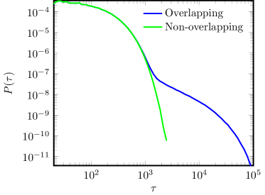
Figure 1: Influence of overlapping defect potentials on the pinning time distribution for single line elements ($L=1$) in the free-flowing phase. The blue (dark) graph shows data from simulations in which discrete pinning potential wells were allowed to overlap, while the green (light) curve displays results for strictly non-overlapping sites. Simulation parameters: $T=0.02\epsilon_{0}b_{0}$, $F=0.002\epsilon_{0}b_{0}^{-1}$, $N_{k}=50$, $\mu=0.1\epsilon_{0}$, $w=0.001\epsilon_{0}$; the data were averaged over $1000$ independent realizations.

Before we investigate the resulting pinning time distributions in detail, we briefly address the influence of overlapping discrete potential wells. A uniformly random positioning of pinning sites inevitably leads to spatially overlapping defect potentials. This, of course, generates regions where the disorder potential is considerably stronger than for single pins. Figure 1 shows the effects of overlapping sites on $P(\tau)$ in the free-flowing phase. The pinning time distribution exhibits two successive humps if overlapping sites are allowed. The second flat region disappears when existing pinning centers are strictly avoided during the placement of new sites. We interpret the data for the potentially overlapping pins as reflecting a two-step process: When a line element is trapped inside an isolated site with typical depth $U_{1}\approx\mu$, its escape time is on the order of $\tau_{1}\sim 10^{2}t_{0}$. When overlaps are prohibited, this is the only relevant time scale. Yet in the presence of overlapping wells, there exist regions with a disorder potential that, on average, is twice as deep as single sites, $U_{2}\approx 2\mu$. Line elements trapped in such deeper troughs require a much longer time $\tau_{2}$ to leave the trap. From Fig. 1, we infer $\tau_{2}\approx\tau_{1}^{2}\sim 10^{4}t_{0}$, which is consistent with Kramers’ solution for the escape time problem, wherein the mean escape time is proportional to $\exp(-U/T)$. In Ref. Lama2009 , the authors similarly observe multiple plateaus in the activity statistics of elastic strings at low temperatures. In the remainder of this article, pinning site overlaps are explicitly disallowed.

V Simulation Results

V.1 Pinned versus free-flowing phase

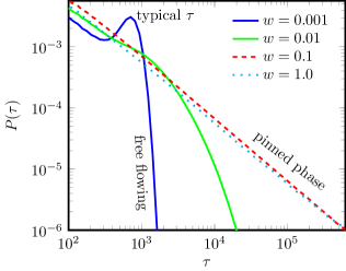
Figure 2: Pinning time distribution $P(\tau)$ for discrete pinning sites for varying standard deviation $w$ of the pin strength, both in the pinned and moving phases, at fixed parameter values $L=200$, $T=0.002\epsilon_{0}b_{0}$, $F=0.002\epsilon_{0}b_{0}^{-1}$, $N_{k}=100$, and $\mu=0$. The local maximum of $P(\tau)$ deep in the freely flowing phase indicates a characteristic pinning time. For each parameter set, the data were averaged over $1000$ independent realizations.

We first explore the dynamic transition between the pinned and free-flowing phases of driven vortex lines at the critical depinning force $F_{c}$, which is a function of the Larkin–Ovchinnikov length $L_{L}$ and hence depends on defect potential properties, specifically the disorder strength variance $w^{2}$. For the numerical data displayed in Fig. 2, we held the driving force (as well as all other parameters) fixed but varied $w$ for a system with randomly distributed discrete point-like pins (6). For large values of the disorder strength variance, the pinning time distribution exhibits power law behavior. For small values of $w$, one instead observes $P(\tau)$ to become a quickly decaying function once $\tau>1000t_{0}$, indicating that the elastic lines are freely flowing. The pronounced local maximum visible near $\tau\approx 700t_{0}$ for $w=0.001\epsilon_{0}$ marks a characteristic average time for a line element to traverse a pinning site of radius $b_{0}$. We estimate the critical disorder variance at applied force $F=0.002\epsilon_{0}b_{0}^{-1}$ as $w_{L}\approx 0.01\epsilon_{0}$, wherefrom we may infer $\xi=w_{L}^{4/3}/(\epsilon^{1/3}F)\approx 1.88b_{0}$. This disorder correlation length value matches the numerically determined mean nearest-neighbor distance between pinning sites $d\approx 2.7b_{0}$ and the pinning center radius $b_{0}$. We have also studied samples with purely attractive pinning sites, i.e., truncated Gaussian disorder distributions with width $w$ limited to $p^{(i)}_{k}<0$. In the moving phase, the resulting graph for $P(\tau)$ coincides with the corresponding blue (dark) curve for $w=0.001\epsilon_{0}$ in Fig. 2; in the pinned state, $P(\tau)$ is merely parallel-shifted (upwards by a factor $\approx 1.5$) from the dashed red line for $w=0.1\epsilon_{0}$ in Fig. 2 (data not shown).

V.2 Pinning time statistics for discrete disorder

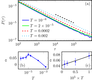
Figure 3: (a) Pinning time distribution $P(\tau)$ for discrete pinning sites at different temperatures $T$ in the pinned state, with parameters $L=200$, $F=0.002\epsilon_{0}b_{0}^{-1}$, $N_{k}=100$, $\mu=0$, and $w=\epsilon_{0}$. (b) Decay exponent $\alpha(T)$ as defined in Eq. (3) as a function of temperature, obtained by fitting in the region indicated by the black dashed line in (a). (c) Linear plot of $\alpha(T)$ for low temperatures $T\leq 10^{-5}\epsilon_{0}b_{0}$. The solid line represents the linear fit function $\alpha(T)=0.0417+3340\,T$. The data were generated from $10^{4}$ realizations for each parameter set, except for $T=0.002\epsilon_{0}b_{0}$, for which $1000$ realizations were used.

We next address the scaling properties of the dwelling time distribution $P(\tau)$ for vortex lines that are pinned to discrete localized potential wells (6) with mean strength $\mu=0$ and variance $w^{2}$ under the influence of a subcritical driving force $F<F_{c}$. Figure 3(a) shows the pinning time distribution for $w=\epsilon_{0}$ and $F=0.002\epsilon_{0}b_{0}^{-1}$, i.e., in the pinned phase, at various temperatures. Beyond $\tau\approx 10^{3}t_{0}$, $P(\tau)$ settles to a power law decay over two decades. This is followed by a crossover to a different long-time regime for $\tau>10^{5}t_{0}$. We have extracted the scaling exponent $-(1+\alpha)$ from Eq. (3) in the intermediate time regime $10^{4}t_{0}<\tau<10^{5}t_{0}$ by a linear fit to the double-logarithmic data. The resulting decay exponent $\alpha(T)$ as function of temperature is plotted in Fig. 3(b). This graph exhibits two distinct regimes: For $T\leq 10^{-5}\epsilon_{0}b_{0}$ we observe approximately linear growth, whereas $\alpha(T)$ decreases above this threshold and even appears to become negative close to the depinning transition. Our data do not confirm the prediction of Ref. Vinokur1996 that $\alpha\to 1$ as $T$ approaches the critical depinning temperature. The simple power law (3) should be valid in the limit $T\to 0$ where the energy scales are not significantly renormalized by thermal fluctuations; hence one expects $\alpha(T)\propto T$ for low temperatures Vinokur1996 . Figure 3(c) provides a linear plot for $\alpha(T)$ in the low-temperature region $T\leq 10^{-5}\epsilon_{0}b_{0}$. We indeed find an approximately linear relationship with a proportionality factor $3340(\epsilon_{0}b_{0})^{-1}$. However, the apparent nonzero intercept $\alpha(T\to 0)\approx 0.042$ is incompatible with Eq. (3).

V.3 Attractive pins versus mixed repulsive and attractive defects

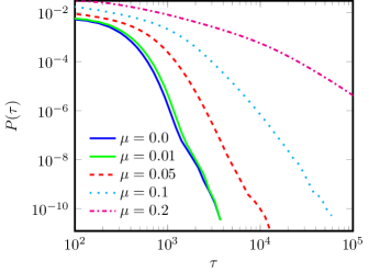
Figure 4: Pinning time distributions $P(\tau)$ for different mean disorder strengths $\mu$ of discrete defect sites in a one-dimensional transverse domain ($l=3400b_{0}$ and $W=0$) for parameter values $L=200$, $T=0.02\epsilon_{0}b_{0}$, $F=0.002\epsilon_{0}b_{0}^{-1}$, $N_{k}=50$, and $w=0.001\epsilon_{0}$. Data in this figure were generated from a minimum of $6500$ realizations for each set of parameter values.

Here we wish to explore differences between largely attractive and a mixture of repulsive and attractive disorder. Yet in a sample with two available dimensions perpendicular to the directed lines, vortex segments can simply slide past any localized circular repulsive defects. Hence we restrict line movement to one perpendicular dimension in this section. Figure 4 displays the pinning time distribution for discrete defects for various mean disorder potential strengths $\mu$ at fixed low standard deviation $w=0.001\epsilon_{0}$. In the symmetric case $\mu=0$, defect wells have an equal chance of being attractive and repulsive, while for finite $\mu>0$, fewer repulsive sites are present. It is obvious from the graphs that upon increasing $\mu$, characteristic pinning times become longer due to the prevalence of deeper potential wells, and one observes a gradual crossover from the freely moving vortex state into the pinned phase. This behavior cannot be realized with a Gaussian disorder landscape, since a shift in the Gaussian distribution merely adds an additive constant to the Hamiltonian which is irrelevant for the dynamics.

V.4 Pinning Potential Landscape

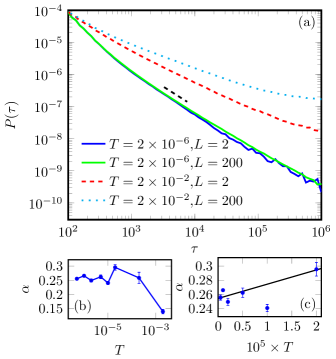
Figure 5: (a) Pinning time distributions $P(\tau)$ for a continuous Gaussian disorder landscape with $\xi=b_{0}$ and different line lengths $L$ and temperatures $T$, and parameter values $F=0.002\epsilon_{0}b_{0}^{-1}$ and $w=\epsilon_{0}$. (b) Decay exponent $\alpha(T)$ as function of temperature for $L=200$, obtained by fitting in the region indicated by the black dashed line in (a). (c) Linear plot of $\alpha(T)$ for low temperatures $T\leq 2\times 10^{-5}\epsilon_{0}b_{0}$. The solid line represents the linear fit function $\alpha(T)=0.2542+2019\,T$ (excluding the outlying data point at $T=10^{-5}\epsilon_{0}b_{0}$). The data were generated from $2\times 10^{4}$ independent realizations for each parameter set for $T<2\times 10^{-5}\epsilon_{0}b_{0}$, else from $1000$ realizations.

We finally investigate the scaling properties of the dwelling time distribution in the pinned phase when disorder is implemented through a continuous Gaussian potential landscape. Figure 5(a) shows the resulting distributions $P(\tau)$ for different temperatures and line lengths $L=2$ and $L=200$, allowing a direct comparison with the data in Fig. 3 obtained for discrete pinning sites with identical driving force $F=0.002\epsilon_{0}b_{0}^{-1}$ and disorder strength standard deviation $w=\epsilon_{0}$. Once again we observe a crossover from an early-time to the algebraic decay regime, but now around $\tau\approx 10^{2}t_{0}$, indicating a different overall energy scale. We note that at low temperatures, no difference in the distribution of pinning times between long and short vortex lines is discernible. For large temperatures, however, cooperative effects between the line elements come into play that effectively enhance the pinning times for long elastic lines. The decay exponent $\alpha(T)$ as function of temperature is plotted in Fig. 5(b), here acquired by fitting a power law to the data in the region indicated by the black dashed line in (a). The decay exponent values for a continuous pinning landscale are significantly enhanced by a factor $\approx 4\ldots 6$ in comparison with discrete pinning sites, and strictly positive for the temperature range investigated here. For small temperatures $T\leq 2\times 10^{-5}\epsilon_{0}b_{0}$, $\alpha(T)$ is again well described by a linear function of $T$, with a definitely positive zero-temperature limit $\alpha(T\to 0)\approx 0.254$.

VI Conclusions

We have employed a directed elastic line model and utilized Langevin molecular dynamics to investigate the pinning kinetics of driven non-interacting magnetic vortices in type-II superconductors subject to point defects. We have focused specifically on the pinning time distribution $P(\tau)$ and its scaling properties in the pinned state. We have elucidated similarities and differences between distinct disorder implementations: (i) discrete pinning sites with localized spherical potential wells (6), whose strengths were drawn from a normal distribution with mean $\mu$ and standard deviation $w$, and which were randomly distributed in the simulation domain, aside from carefully avoiding any spatial overlaps of the wells; and (ii) continuous Gaussian disorder landscapes, correlated on a length scale $\xi$ and again with variance $w^{2}$.

For discrete pinning sites, we found very similar dwelling time distribution shapes for either purely attractive or symmetric defect potentials with $\mu=0$ in our samples with two transverse dimensions. Restricting line motion to merely one transverse direction, increasing the mean $\mu$ induces a very gradual crossover from the moving to the pinned state. In contrast, upon increasing the disorder distribution width $w$ at fixed $\mu=0$ (as well as driving force $F$ and temperature $T$) in the fully three-dimensional samples, one observes a sharp transition between the freely flowing and pinned vortex phases. Thus we could extract a reasonable value for the disorder correlation length $\xi$ from the Larkin–Ovchinnikov collective pinning picture.

In the pinned phase, the dwelling time statistics for the elastic line elements decays algebraically, cf. Eq. (3) as predicted in Ref. Vinokur1996 , with a decay exponent $\alpha(T)$ that is well approximated by a growing linear function at very low temperatures, but which decreases with $T$ beyond a remarkably sharp threshold temperature. Both this threshold and the numerical values of $\alpha$ strongly depend on the disorder implementation: For the continuous random potential landscape, the former is enhanced by about a factor $2$ for our chosen parameter values, and the latter by roughly $5$ as compared to corresponding systems with discrete pins. We also observe that the zero-temperature extrapolation $\alpha(T\to 0)$ yields a positive value, indicating perhaps subtle renormalization effects not entirely captured in the analysis of Ref. Vinokur1996 .

In-depth studies of the dwelling time statistics in disordered systems thus reveal remarkably rich features that offer novel insights in the associated subtle physical interplay between competing energy scales. A natural extension of the present study would be to incorporate mutual repulsive forces between vortex lines. Unfortunately, our currently available computing power does not yet allow us to tackle this intriguing issue with satisfactory statistics. Investigating the pinning time statistics for samples with spatially correlated disorder such as columnar or planar defects is also a promising avenue for future research. Because of much more efficient pinning of vortex lines in the presence of extended defects, we expect the associated time scales to grow and temporal correlations to play a significant role. This renders such extended studies quite challenging, at least with our currently available computational resources. Yet we hope to be able to revisit this intriguing problem with its many competing energy scales and associated rich dynamical properties in the future.

- (1) D. S. Fisher, Phys. Rep. 301, 113 (1998).
- (2) S. Brazovskii and T. Nattermann, Adv. Phys. 53, 177 (2004).
- (3) G. Blatter, V. B. Geshkenbein, A. I. Larkin, and V. M. Vinokur, Rev. Mod. Phys. 66, 1125 (1994).
- (4) L. B. Ioffe and V. M. Vinokur, J. Phys. C.: Solid State Phys. 20, 6149 (1987).
- (5) D. Ertaş and M. Kardar, Phys. Rev. Lett. 69, 929 (1992).
- (6) D. Ertaş and M. Kardar, Phys. Rev. B 53, 3520 (1996).
- (7) M. Kardar, Phys. Rep. 301, 85 (1998).
- (8) T. Halpin-Healy and Y-C. Zhang, Phys. Rep. 254, 215 (1995).
- (9) A. Rosso, A. K. Hartmann, and W. Krauth, Phys. Rev. E 67, 021602 (2003).
- (10) E. Agoritsas, V. Lecomte, and T. Giamarchi, Physica B 407, 1725 (2012).
- (11) X. Du, G. Li, E. Y. Andrei, M. Greenblatt, and P. Shuk, Nat. Phys. 3, 111 (2007).
- (12) M. Pleimling and U. C. Täuber, Phys. Rev. B 84, 174509 (2011).
- (13) U. Dobramysl, H. Assi, M. Pleimling, and U. C. Täuber, Eur. Phys. J. B 86, 1 (2013).
- (14) H. Assi, U. Dobramysl, M. Pleimling, and U. C. Täuber, in preparation.
- (15) T. Nattermann and S. Scheidl, Adv. Phys. 49, 607 (2000).
- (16) A. B. Kolton, A. Rosso, T. Giamarchi, and W. Krauth, Phys. Rev. B 79, 184207 (2009).
- (17) O. Duemmer and W. Krauth, Phys. Rev. E 71, 061601 (2005).
- (18) C. J. Bolech and A. Rosso, Phys. Rev. Lett. 93, 125701 (2004).
- (19) S. Bustingorry, A. B. Kolton, and T. Giamarchi, Phys. Rev. B 82, 094202 (2010).
- (20) V. M. Vinokur, M. C. Marchetti, and L.-W. Chen, Phys. Rev. Lett. 77, 1845 (1996).
- (21) D. R. Nelson and V. M. Vinokur, Phys. Rev. B 48, 13060 (1993).
- (22) A. Brass and H. J. Jensen Phys. Rev. B 39, 9587 (1989).
- (23) J. Bardeen and M. J. Stephen, Phys. Rev. 140, A1197 (1965).
- (24) J. L. Iguain, S. Bustingorry, A. B. Kolton, and L. F. Cugliandolo, Phys. Rev. B 80, 094201 (2009).
- (25) M. S. de la Lama, J. M. López, J. J. Ramasco, and M. A. Rodríguez, J. Stat. Mech. 2009, P07009 (2009).