Star formation history, dust attenuation and extragalactic background light

Abstract

At any given epoch, the Extragalactic Background Light (EBL) carries imprints of integrated star formation activities in the universe till that epoch. On the other hand, in order to estimate the EBL, when direct observations are not possible, one requires an accurate estimation of the star formation rate density (SFRD) and the dust attenuation ($A_{\nu}$) in galaxies. Here, we present a ‘progressive fitting method’ that determines the global average SFRD($z$) and $A_{\nu}$($z$) for any given extinction curve by using the available multi-wavelength multi-epoch galaxy luminosity function measurements. Using the available observations, we determine the best fitted combinations of SFRD($z$) and $A_{\nu}$($z$), in a simple fitting form, up to $z\sim 8$ for five well known extinction curves. We find, irrespective of the extinction curve used, the $z$ at which the SFRD($z$) peaks is higher than the $z$ above which $A_{\nu}$($z$) begins to decline. For each case, we compute the EBL from ultra-violet to the far-infrared regime and the optical depth ($\tau_{\gamma}$) encountered by the high energy $\gamma$-rays due to pair production upon collisions with these EBL photons. We compare these with measurements of the local EBL, $\gamma$-ray horizon and $\tau_{\gamma}$ measurements using Fermi-LAT. All these and the comparison of independent SFRD($z$) and $A_{\nu}$($z$) measurements from the literature with our predictions favor the extinction curve similar to that of Large Magellanic cloud Supershell.

1. Introduction

The extragalactic background light (EBL) at any epoch is a diffuse isotropic background radiation, defined here over the wavelength range 0.1 to 1000$\mu$m excluding the cosmic microwave background radiation (CMBR), believed to be contributed mainly by the sources such as galaxies and QSOs. The knowledge of how the intensity and shape of the EBL evolves is very important for understanding the galaxy evolution in the universe.

Direct measurements of the EBL are possible only in the local universe (Dwek & Arendt, 1998; Dole et al., 2006; Matsuoka et al., 2011). However, there are large uncertainties associated with the removal of foreground contributions from the unresolved point sources and zodiacal light (see Hauser & Dwek, 2001). The local EBL can be inferred by adding the light from resolved sources (Madau & Pozzetti, 2000; Xu et al., 2005; Hopwood et al., 2010) but the convergence of the number of sources is in dispute (Bernstein et al., 2002; Levenson & Wright, 2008). However, with the aid of rapidly developing $\gamma$-ray astronomy, in principle, it is possible to place strong constraints on the intermediate redshift (z$<$2) EBL.

The high energy $\gamma$-rays by interacting with the EBL photons can annihilate themselves and produce electron positron pairs. The byproduct of this interaction, ultra-relativistic electron positron pairs, are expected to inverse Compton scatter the CMBR and produce secondary $\gamma$-rays. These secondary $\gamma$-rays are not yet detected by the Fermi satellite implying either the presence of a small intergalactic magnetic field that scatters the produced pairs (Neronov & Vovk, 2010; Tavecchio et al., 2011; Takahashi et al., 2012; Arlen et al., 2012) or the electromagnetic pair cascade dissipating pair beam energy in to the intergalactic medium (IGM; see for e.g., Schlickeiser et al., 2013; Miniati & Elyiv, 2013). Nevertheless, this process of pair production attenuates the $\gamma$-rays originating from distant sources while traveling through the IGM (Gould & Schréder, 1966; Jelley, 1966). The amount of attenuation suffered by the $\gamma$-rays emitted by sources at different emission redshifts depends on the number density of the EBL photons encountered while traveling from the source to the earth. Thus a well measured $\gamma$-ray attenuation ($\tau_{\gamma}$) can be used to put constraints on the evolution of the shape and amplitude of the EBL. This was initially suggested by Stecker et al. (1992) and the first few limits on the IR part of the EBL were placed by Dwek & Slavin (1994) and de Jager et al. (1994) using TeV $\gamma$-ray observations of the blazar Mrk 421.

With the aid of new generation ground based $\gamma$-ray Imagining Atmospheric Cherenkov telescopes (IACT) and the Fermi satellite, many high energy $\gamma$-ray sources have been detected. The observed spectrum of distant $\gamma$-ray sources are used to determine the $\tau_{\gamma}$. However, the difficulty in doing so arises from the fact that the intrinsic spectral energy distribution (SED) of each source is unknown. Recently, Ackermann et al. (2012) have circumvent this difficulty and reported the measurements of $\tau_{\gamma}$ up to $z\sim 1.5$ with the observed $\gamma$-ray energies from 10 to 500 GeV using the stacked spectra of $\gamma$-ray blazars selected from the sample of objects observed with Large Area Telescope (LAT) on board the Fermi satellite. It is expected to find the $\tau_{\gamma}$ increasing with increasing redshift since these $\gamma$-rays travel longer distances through EBL photons to reach earth. The observation of this cosmological evolution in $\tau_{\gamma}$ has been reported recently by Sanchez et al. (2013). The $\gamma$-ray horizon for $\gamma$-ray photons with the observed energy $E_{\gamma}$ is defined as the emission redshift of $\gamma$-rays beyond which they encounter $\tau_{\gamma}>1$. Recently, by using a physically motivated modeling of intrinsic SEDs of 15 blazars, Domínguez et al. (2013) reported the $\gamma$-ray horizon measurements. Domínguez & Prada (2013) using such $\gamma$-ray horizon measurements have demonstrated the capability of $\gamma$-ray astronomy to measure the Hubble constant. Recently, Scully et al. (2014) and Stecker et al. (2012) used their EBL model to constrain the redshift of $\gamma$-ray blazars. In some sense, the backbone of this rapidly developing $\gamma$-ray astronomy is the EBL. Therefore, it is very important to have an EBL estimates consistent with different observations over a large redshift range.

To estimate the EBL one needs the specific emissivity (or some times referred as luminosity density) at each frequency and redshift. The EBL in optical wavelengths is predominantly contributed by the stellar emission and in the infra-red (IR) wavelengths by dust emission from galaxies. Therefore, for the correct estimation of the EBL one has to determine the comoving specific galaxy emissivity at different frequencies and redshifts, $\rho_{\nu}(z)$, as accurately as possible. The EBL models are generally classified in to different categories depending on the method adopted to get the $\rho_{\nu}(z)$. For example, some of the models, say the first kind of models, start with simulating the galaxy evolution in the framework of standard cosmological model taking into account the dark matter halo formation and some prescription to relate baryons to star formation in them. These models then predict the $\rho_{\nu}(z)$ forward in time (Primack et al., 2005; Gilmore et al., 2009, 2012; Inoue et al., 2013). There are second type of models which construct the grid of $\rho_{\nu}(z)$ measurements in different wavebands and redshift and then apply the interpolation and the extrapolation to get the $\rho_{\nu}(z)$ at each $\nu$ and $z$ (Stecker et al., 2006; Franceschini et al., 2008; Domínguez et al., 2011; Stecker et al., 2012; Helgason & Kashlinsky, 2012). There are third kind of models where the cosmic star formation history and the SED of stellar population of galaxies are convolved to get the $\rho_{\nu}(z)$ (Kneiske et al., 2004; Finke et al., 2010; Haardt & Madau, 2012). The $\rho_{\nu}(z)$ obtained in this way depends on star formation history of galaxies over the cosmic time and absorption and scattering by the dust present in them. Main uncertainties in the first and third approach are related to the the amount of dust corrections which is usually quantified by the dust attenuation magnitude $A_{\nu_{0}}$ at frequency $\nu_{0}$ and a wavelength dependent dust extinction curve. It is a general practice to assume a form of $A_{\nu_{0}}(z)$ and an extinction curve to get the $\rho_{\nu}(z)$ from the star formation history. Irrespective of the approach one adopts, all the methods are expected to reproduce the measured $\rho_{\nu}(z)$ using observed luminosity functions.

Here, in this paper, we address the issue of self consistently determining the dust correction and the star formation history which will reproduce the observed emissivity. We present a novel ‘progressive fitting method’ which by using the $\rho_{\nu}(z)$, for a given extinction curve, determines a unique combination of cosmic star formation rate density (SFRD) and $A_{\nu_{0}}(z)$. We apply this method on observationally determined $\rho_{\nu}(z)$ using the available multi-wavelength multi-epoch galaxy data from the literature. We determine the combinations of SFRD($z$) and $A_{\nu_{0}}(z)$ for a set of five well known extinction curves and compare the results with different independent measurements of SFRD($z$) and $A_{\nu_{0}}(z)$ available in the literature. This allows us to determine the average extinction curve that can be used to convert the emissivity into the SFRD($z$). We provide the simple fitting forms of these combinations of SFRD($z$) and $A_{\nu_{0}}(z)$ for each extinction curve with their $1\sigma$ upper and lower limits. We self-consistently determine the amount of stellar light absorbed by dust with the help of these combinations of $A_{\nu_{0}}(z)$ and SFRD($z$) obtained for different extinction curves and then estimate the far infra-red (FIR) emission from galaxies using the local galaxy FIR templates and the energy conservation arguments. In this way we obtain the specific emissivity from UV to FIR and then use standard prescription to calculate the EBL, the $\tau_{\gamma}$ and the $\gamma$-ray horizon and compare these results with different available measurements. We conclude that the combination of $A_{\nu_{0}}(z)$ and SFRD($z$) obtained using the extinction curve of Large Magellanic cloud Supershell (LMC2) and the inferred local FIR emissivity are consistent with the different measurements and we call the EBL obtained using it as our fiducial model for the EBL. The EBL obtained in this way, by exploring different well known extinction curves and corresponding combinations of self-consistent $A_{\nu_{0}}(z)$ and SFRD($z$), includes better treatment of dust correction and gives a general picture of how the FIR part of the EBL depends on it.

The outline of this paper is as follows. In section 2 we present the standard radiative transfer equation used for calculating the EBL from the inferred emissivities. In section 2.1, we describe the QSO contribution to the total emissivity used by us. In section 2.2, we describe the standard procedure to get the galaxy emissivity using the SFRD($z$) and $A_{\nu_{0}}(z)$. In section 3, we summarize the galaxy emissivity measurements from the literature that we use in our study and describe our ‘progressive fitting’ technique which determines a unique combination of $A_{\nu_{0}}(z)$ and SFRD($z$) for an assumed extinction curve. In section 4, we make a detailed comparison of SFRD($z$) and $A_{\nu_{0}}(z)$ obtained using our technique for five different extinction curves with those determined from the independent observations. We explain in detail the method used by us to calculate the FIR emissivity from galaxies in section 5. Then we use these inferred galaxy emissivities to calculate the EBL at different $z$. We present our EBL predictions and compare them with the other EBL estimates from the literature in section 6. In section 7, we describe the basics of the pair production mechanism used for calculating the $\tau_{\gamma}$ for our EBL models and compare our results with the other independent measurements. We conclude with the discussion related to the uncertainties in estimating the star formation history, $A_{\nu_{0}}(z)$ and the EBL in section 8 and summarize the results in section 9. Throughout the paper we use cosmology with $\Omega_{\lambda}$=0.7, $\Omega_{m}$=0.3 and $H_{0}$=70 km s^-1 Mpc^-1.

2. Cosmological radiative transfer

In this section, we provide a general outline for the basic EBL calculations. The number density of background photons at a frequency $\nu_{0}$ and redshift $z_{0}$ is given by,

$$n(\nu_{0},z_{0})=\frac{4\pi J_{\nu_{0}}(z_{0})}{hc}\,\,,$$ (1)

where, $h$ is the Planck’s constant and $J_{\nu_{0}}$ is the specific intensity of the EBL (in units of erg cm${}^{\text{-2}}$ s${}^{\text{-1}}$ Hz${}^{\text{-1}}$ sr${}^{\text{-1}}$) at a frequency $\nu_{0}$. Following the standard procedure (see for example, Haardt & Madau, 2012, referred as HM12 from now onwards), we assume that the QSOs and galaxies are the sole contributers to the EBL at all wavelengths. We do not consider contributions to the EBL from the non-standard sources like decaying dark matter or dark energy. From the observed luminosity functions of QSOs and galaxies at a redshift $z$ and a frequency $\nu$ one can calculate the proper space averaged specific volume emissivity $\epsilon_{\nu}(z)$ (in units of erg s${}^{\text{-1}}$ Hz${}^{\text{-1}}$ Mpc${}^{\text{-3}}$). Then, the radiative transfer equation, which gives the specific intensity $J_{\nu_{0}}(z_{0})$ of the EBL as seen by an observer at a redshift $z_{0}$ and a frequency $\nu_{0}$, can be written as (Peebles, 1993; Haardt & Madau, 1996),

$$J_{\nu_{0}}(z_{0})=\frac{1}{4\pi}\int_{z_{0}}^{\infty}dz\,\frac{dl}{dz}\,\frac{(1+z_{0})^{3}}{(1+z)^{3}}\,\epsilon_{\nu}(z)\,e^{-\tau_{eff}(\nu_{0},z_{0},z)}.$$ (2)

Here, $\frac{dl}{dz}$ is the cosmological Freidmann-Robertson-Walker (FRW) line element, the $\nu=\nu_{0}(1+z)/(1+z_{0})$ is a frequency of the radiation originated from a redshift $z$ and $\tau_{eff}(\nu_{0},z_{0},z)$ is the effective IGM optical depth encountered by the radiation emitted at a frequency $\nu$ while traveling through the IGM from an emission redshift $z$ to a redshift $z_{0}$ where it has been observed at a frequency $\nu_{0}$. The hydrogen and helium gas present in the IGM and in galaxies dominate $\tau_{eff}$ at $\lambda\leq 0.091\mu$m through the photo-absorption. However, in the optical wavelengths it was believed that the main contribution to the opacity comes from the attenuation by the dust associated with high H i column density intervening systems. Based on the available QSO spectroscopic observations one can conclude that this effect is indeed negligible (see, Srianand & Kembhavi, 1997; York et al., 2006; Frank & Péroux, 2010; Khare et al., 2012; Ménard & Fukugita, 2012). Here, as we are interested in calculating the EBL at $\lambda>$ 0.1$\mu m$, we will consider $\tau_{eff}$=0 in Eq. 2. This assumption has negligible effect on the computed EBL and it does not affect the $\tau_{\gamma}$ significantly over the $\gamma$-ray energy range of our interest.

2.1. QSO contribution to emissivity

The proper specific volume emissivity of the radiating sources can be written as,

$$\epsilon_{\nu}(z)=\epsilon_{\nu,\rm Q}(z)+\epsilon_{\nu,\rm G}(z)\,\,,$$ (3)

where, $\epsilon_{\nu,\rm Q}(z)$ and $\epsilon_{\nu,\rm G}(z)$ are the proper specific volume emissivity of QSOs and galaxies, respectively. For QSOs, we use the parametric form for $\epsilon_{\nu,\rm Q}(z)$ as given in HM12 at $912\text{\AA}$ which is consistent with the QSO luminosity function of Hopkins et al. (2007),

$$\frac{\epsilon_{912,\rm Q}(z)}{(1+z)^{3}}=10^{24.6}\,(1+z)^{4.68}\,\frac{exp(-0.28z)}{exp(1.77z)+26.3}\,\,\,,$$ (4)

in units of ergs s${}^{\text{-1}}$ Mpc${}^{\text{-3}}$ Hz${}^{\text{-1}}$. To get $\epsilon_{\nu,\rm Q}$ at different wavelengths, we use a SED given by the broken power law, $L_{\nu}\propto\nu^{-0.44}$ for $\lambda>$1300Å and $L_{\nu}\propto\nu^{-1.57}$ for $\lambda<$1300Å (Vanden Berk et al., 2001; Telfer et al., 2002). It is well known that the stellar emission from galaxies dominate the EBL in the optical regime in all redshifts. Therefore, we place more emphasis on the estimating $\epsilon_{\nu,\rm G}(z)$ accurately. We discuss this in detail in the following section.

2.2. Galaxy contribution to emissivity

Table 1Details of the observed galaxy luminosity functions used to get the $\rho_{\nu}$ in our study.

Reference	Waveband∗	Redshift range	Plotting Symbol†
Schiminovich et al. (2005)	FUV	0.2-2.95	magenta triangle
Reddy & Steidel (2009)	FUV	1.9-3.4	orange triangle
Bouwens et al. (2007)	FUV	3.8-5.9	Red diamond
Bouwens et al. (2011)	FUV	6.8-8	Red diamond
Dahlen et al. (2007)	FUV	0.92-2.37	blue square
	NUV	0.29-2.37	blue square
Cucciati et al. (2012)	FUV	0.05-4.5	green circle
	NUV	0.05-3.5	green circle
Tresse et al. (2007)	FUV, NUV, U, V, B, R, I	0.05-2	red circle
Wyder et al. (2005)	NUV	0.055	black triangle
Faber et al. (2007)	B	0.2-1.2	orange star
Dahlen et al. (2005)	U, B, R	0.1-2	blue square
	J	0.1-1	blue square
Stefanon & Marchesini (2013)	J, H	1.5-3.5	green square
Pozzetti et al. (2003)	J, K	0.2-1.3	orange triangle
Arnouts et al. (2007)	K	0.2-2	green diamond
Cirasuolo et al. (2007)	K	0.25-2.25	blue triangle

^∗Central wavelengths corresponding to different wavebands are as follows: FUV=0.15$\mu$m, NUV=0.28$\mu$m, U=0.365$\mu$m, B=0.445$\mu$m, V=0.551$\mu$m, R=0.658$\mu$m, I=0.806$\mu$m, J=1.27$\mu$m, H=1.63$\mu$m and K=2.2$\mu$m.
^† These plotting symbols are used in Fig. 5 and Fig. 17 for the $\rho_{\nu}$ obtained using different luminosity functions.

We need to compute the galaxy emissivity, $\epsilon_{\nu,\rm G}(z)$, which is consistent with the observed luminosity functions of galaxies at different wavelengths and redshifts. The luminosity function, $\phi_{\nu}(L,z)$, observed at different $z$ and frequency $\nu$ is usually specified in the form of Schechter function. The comoving luminosity density, $\rho_{\nu}(z)$, for galaxies which is nothing but the space averaged comoving specific emissivity,

$$\rho_{\nu}(z)=\frac{\epsilon_{\nu,\rm G}(z)}{(1+z)^{3}}\,\,,$$

is given by an integral,

$$\rho_{\nu}=\int_{L_{min}}^{\infty}{L\phi_{\nu}(L)dL}=\phi_{\nu}^{*}\,\,L^{*}\,\,\Gamma(\alpha+2,\,\,L_{min}/L^{*}).$$ (5)

Here, $\phi_{\nu}^{*}$, $L^{*}$ and $\alpha$ are the Schechter parameters, $L_{min}$ is the luminosity corresponding to faintest galaxy at a redshift $z$ and $\Gamma$ is the incomplete gamma function. We dropped the subscript $z$ in above equation for clarity. The $\rho_{\nu}$ depends on the choice of $L_{min}$. In principle, one can always take $L_{min}=0$ for $\alpha>-2.0$ where the integral in Eq. 5 converges. Generally, for galaxies at $z<2.5$, one finds $\alpha>-1.3$ (Cucciati et al., 2012). In this case, the change in $\rho_{\nu}$, when one changes the $L_{min}$ from 0 to 0.01$L^{*}$, is less than $10\%$. We discuss the effect of adopting different the $L_{min}$ values in section 8.

The $\rho_{\nu_{0}}(z)$ measurements are used to determine the global star formation history (see Madau et al., 1996; Lilly et al., 1996) of the universe provided that the magnitude of the dust attenuation, $A_{\nu_{0}}(z)$, at any frequency $\nu_{0}$ and redshift $z$ is known. The average star formation rate density (SFRD), in units of M_⊙ yr^-1 Mpc^-3, is connected to $\rho_{\nu_{0}}$ through the relationship (Kennicutt, 1998),

$$\text{SFRD}(z)=\zeta_{\nu_{0}}\times\rho_{\nu_{0}}(z)10^{0.4A_{\nu_{0}}(z)}.$$ (6)

Here, $\zeta_{\nu_{0}}$ is a constant conversion factor which depends on $\nu_{0}$ and the initial mass function (IMF) assumed for galaxies. However, note that the relation given in Eq. 6 is an approximation as $\rho_{\nu_{0}}(z)$ can also have contributions from the old stellar population where the stars that are formed earlier are still shining at $z$.

The derived SFRD($z$) and the SED produced from the instantaneous burst of star formation can be used to get the luminosity density at different $\nu$ and $z$. For an assumed initial mass function (IMF) and metallicity $Z$, the population synthesis models provide a SED in terms of specific luminosity, $l_{\nu}(\tau,Z)$, (in units of ergs s^-1 Hz^-1 per unit mass of stars formed) at different age $\tau$ of the stellar population. Since the timescales involved in the process of star formation (10⁵ to 10⁷ years) are relatively small, the SED from the instantaneous star burst can be directly convolved with the global SFRD($z$) to get the $\rho_{\nu}(z_{0})$ by solving the following convolution integral (see for eg, Kneiske et al., 2002, HM12),

$$\rho_{\nu}(z_{0})=C_{\nu}(z_{0})\int_{z_{0}}^{z_{max}}{\rm SFRD}(z)\,\,l_{\nu}[t(z_{0})-t(z),Z]\,\,\frac{dt}{dz}\,\,dz\,,$$ (7)

where, the $\tau=t(z_{0})-t(z)$ is an age of the stellar population at the redshift $z_{0}$ which went through an instantaneous burst of star formation at a redshift $z$ , $C_{\nu}(z_{0})$ is the dust correction factor at $z_{0}$ and $\frac{dt}{dz}=[(1+z)H(z)]^{-1}$. The fact that the burst of star formations occurs at all epochs, $t$, but with the average star formation rates equals to the global SFRD$(t)$ is captured by the product of ${\rm SFRD}(z)$ and $l_{\nu}[t(z_{0})-t(z),Z]$ in the convolution integral. We use $z_{max}=\infty$ as often used in the literature (e.g., Gilmore et al., 2009; Inoue et al., 2013, HM12). Later in section 8, we discuss the validity of the $z_{max}=\infty$ assumption and the effect of using different $z_{max}$. The dust correction factor, $C_{\nu}(z_{0})$, for $\lambda<912$Å  is assumed to be equal to the escape fraction of hydrogen ionizing photons from galaxies as given in HM12. For $\lambda>912$Å, we use $C_{\nu}(z_{0})=10^{-0.4\,A_{\nu}(z_{0})}$, where, $A_{\nu}(z_{0})$ which is normalized at $\nu_{0}$ as given by,

$$A_{\nu}(z_{0})=A_{\nu_{0}}(z_{0})\frac{k_{\nu}}{k_{\nu_{0}}}.$$ (8)

Here, $k_{\nu}$ is a frequency dependent dust extinction curve.

Figure 1.— The $\rho_{{}_{\rm FUV}}$ as a function of $z$ fitted with a functional form given in Eq. 9. Solid, dashed and dot-dash curves are the median high and low fits, respectively. Data is taken from the references listed in Table 1 for the FUV band.

3. Method to determine SFRD($z$) and A${}_{\nu_{0}}(z)$

In this sections, we summarize $\rho_{\nu}(z)$ measurements from the literature and the progressive fitting method which determines a unique combination of SFRD($z$) and A${}_{\nu_{0}}(z)$ for an assumed extinction curve using $\rho_{\nu}(z)$. By construct, this combination of SFRD($z$) and A${}_{\nu_{0}}(z)$ reproduces the emissivity measurements.

3.1. Compiled luminosity density measurements

Motivated by the previous works of Stecker et al. (2012) and Helgason et al. (2012), we have compiled available observations of the galaxy luminosity functions and the corresponding $\rho_{\nu}$ at different rest wavelengths and $z$. In Table 1, we have given references along with the rest waveband and a redshift range over which the luminosity functions have been determined. In Table 5 in the Appendix, we list the faint end slopes of luminosity functions with the rest waveband and redshift along with the $L_{min}$ values we used to determine $\rho_{\nu}$. In general, we preferred the references where luminosity functions are determined in different wavebands the from the FUV (centered at $\lambda=0.15\mu$m) to K (2.2$\mu$m) band and with the largest possible coverage in redshift. This compilation has luminosity functions determined in the FUV band up to $z=8$, in the NUV and H band up to $z=3.5$ and for all other bands the measurements are available up to $z\sim 2.5$. We take the $\rho_{\nu}(z)$ with the errors from the references where it is explicitly calculated. We use luminosity functions given in other references and compute $\rho_{\nu}$($z$) (using Eq. 5) with $L_{min}=0.01L^{*}$. Since there are more measurements of the $\rho_{\nu}$ in the FUV band and covering a large $z$ range, we choose $\nu_{0}=\nu_{\rm FUV}$, the frequency we use to determine SFRD($z$) as a frequency corresponding to the FUV band.

3.2. Progressive fitting method

We use a population synthesis model ‘Starburst99’ (Leitherer et al., 1999), to get the specific luminosity from stellar population of a typical galaxy, $l_{\nu}(t,Z)$, at an age $t$ and a metallicity $Z$ with an instantaneous burst of star formation. In these simulations, we consider a constant metallicity of $Z=0.008$ over all $z$. Later in section 8, we also discuss the effect of using different values of metallicity. We use the Salpeter IMF with the exponent of 2.35 and the stellar mass range from 0.1 to 100 M_⊙. For this particular galaxy model, we find the conversion factor for connecting $\rho_{FUV}(z)$ and SFRD($z$) (see Eq. 6) to be $\zeta_{\nu_{0}}=1.25\times 10^{-28}$. As described before, the reference frequency, $\nu_{0}$ which we use corresponds to the frequency of the FUV band. Note that, this conversion factor 1.25$\times 10^{-28}$ is 11% smaller than widely used, 1.4$\times 10^{-28}$, quoted by Kennicutt (1998). This difference is mainly because of the updated population synthesis model and the assumed metallicity.

We fit a functional form to the compiled $\rho_{\rm FUV}$ data and obtained its parameter using the mpfit IDL routine that uses $\chi^{2}$ minimization. At high redshifts, we take 20% errors on the $\rho_{\rm FUV}$ calculated from the luminosity function given by Bouwens et al. (2011). We convert the asymmetric errors into symmetric errors by taking the average of them. To fit $\rho_{\rm FUV}(z)$, we use a following functional form that was originally used by Cole et al. (2001) to fit the SFRD($z$),

$$\rho_{\rm FUV}(z)=\frac{a+bz}{1+(z/c)^{d}}.$$ (9)

There is a large scatter in the $\rho_{\rm FUV}(z)$ data. Therefore, along with this fit (hereafter, median fit) we construct 1-$\sigma$ upper and lower limit fits (hereafter we refer to them as the high and low $\rho_{\rm FUV}$ fits, respectively). These $\rho_{\rm FUV}$ fits multiplied by $1.25\times 10^{-28}$ are nothing but the different SFRD($z$) with the $A_{\text{FUV}}(z)=0$ (see Eq. 6) which are plotted in Fig. 1. The values of fitting parameters for the median $\rho_{\rm FUV}\times 1.25\times 10^{-28}$ fit are $a=(6\pm 1)\times 10^{-2}$, $b=(11\pm 2)\times 10^{-2}$, $c=4.41\pm 0.58$ and $d=3.15\pm 0.62$. We construct 1-$\sigma$ high and low $\rho_{\rm FUV}$ fits by adding and subtracting the error in each parameter from its best fit values, respectively (see, Fig. 1). We determine the combinations of SFRD($z$) and $A_{\rm FUV}(z)$ for all three (low, median and high) $\rho_{\rm FUV}$ fits with different extinction curves as discussed below.

Figure 2.— Extinction curves normalized at the FUV band for SMC, LMC, LMC Supershell (LMC2), Milky-Way (MW) and nearby starburst galaxies by Calzetti et al. (2000). Here, triangles, squares and diamonds represent the mean extinction curve measurements from Gordon et al. (2003) normalized at the FUV band for the SMC, LMC2 and LMC, respectively. Different wavebands are marked with the vertical dashed lines to show the difference in different extinction curves at those wavelengths.

The average extinction curve for high redshift galaxies is one of the key unknowns in the astronomy. However, the mean extinction curves for our galaxy, Small and Large Megallenic Clouds (SMC and LMC) and some low redshift starburst galaxies are well known (Lequeux et al., 1982; Clayton & Martin, 1985; Calzetti et al., 1994). It is a general practice to use the average extinction curve determined for the nearby starburst galaxies by Calzetti et al. (2000) for the high redshift galaxies. Here, along with Calzetti et al. (2000) extinction curve, we use extinction curves determined for SMC, LMC and LMC supershell (LMC2) from Gordon et al. (2003) and Milky-Way (MW) from Misselt et al. (1999). In particular, this set of extinction curves encompasses a wide range of dust properties typically present in the astronomical domain. Since, we are using $\rho_{\rm FUV}$ measurements for determining the SFRD($z$), we normalize all the extinction curves $k_{\nu}$ at $\nu$ corresponding to the FUV band ($0.15\mu$m). In Fig. 2, we have plotted the $k_{\nu}/k_{\text{FUV}}$ for different extinction curves as a function of $\lambda^{-1}$ along with the respective measured data points from Gordon et al. (2003) for the SMC, the LMC and the LMC2. In Fig. 2, we also mark the different $\lambda^{-1}$ for the wavebands at which we have compiled the $\rho_{\nu}$ measurements to determine the $A_{\rm FUV}$ and the SFRD.

From Eq. 6 it is clear that the SFRD($z$) and $A_{\text{FUV}}(z)$ are degenerate quantities and different combinations of them can give the same $\rho_{\text{FUV}}$. However, the measured $\rho_{\nu}$ values at different frequencies other than the FUV band along with the assumed extinction curve break this degeneracy. Here we introduce a novel method that, by using the multi-wavelength and multi-epoch luminosity functions, determines the $A_{\rm FUV}(z)$ and SFRD($z$) uniquely for an assumed extinction curve. In this method we initially fix the $A_{\rm FUV}$ and SFRD at some higher redshifts and then using this we progressively determine $A_{\rm FUV}$ and SFRD at lower redshifts. This ‘progressive fitting method’ is described below in details.

Combining Eq. 6, 7 and 8, the $\rho_{\nu}$($z_{0}$) can be written as,

$$\rho_{\nu}(z_{0})=1.25\times 10^{-28}\times 10^{\big{[}-A_{\rm FUV}(z_{0})\frac{k_{\nu}}{k_{\rm FUV}}\big{]}}$$ (10)

$$\times\int_{z_{0}}^{\infty}\rho_{\rm FUV}(z)\;10^{0.4A_{\rm FUV}(z)}\,l_{\nu}[t(z_{0})-t(z),Z]\,\,\frac{dt}{dz}\,\,dz\,.$$

For a given extinction curve, $k_{\nu}$, and our $\rho_{\rm FUV}(z)$ fits, the only unknown in the above equation is $A_{\rm FUV}(z)$ for $z\geq z_{0}$. Therefore, to get the $\rho_{\nu}$($z_{0}$) one needs to know the $A_{\rm FUV}(z)$ for all $z\geq z_{0}$. The procedure we followed to get the $A_{\rm FUV}(z)$ for each extinction curve $k_{\nu}$ using the $\rho_{\nu}(z)$ measurements is given below:

1. We choose the highest possible redshift $z_{th}$ where we have $\rho_{\nu}(z_{th})$ measurements in most of the wavebands.

2. For all $z\geq z_{th}$, we assume a functional form for $A_{\rm FUV}(z)$.

3. We fix the normalization of this function and hence the value of $A_{\rm FUV}(z_{th})$ by matching the predicted $\rho_{\nu}(z_{th})$ with the measured ones at different wavebands (other than the FUV band) using the least square minimization. This fixes the $A_{\rm FUV}(z)$ for $z\geq z_{th}$. Then we call $z_{th}$ as $z_{1}$.

4. We choose the next redshift $z_{0}<z_{1}$ which is the next nearby lower redshift where we have multi-wavelength $\rho_{\nu}(z_{0})$ measurements.

5. We assume $A_{\rm FUV}(z)$ is constant and equal to $A_{\rm FUV}(z_{0})$ in between the redshifts $z_{0}$ and $z_{1}$. For $z\geq z_{1}$ we use the $A_{\rm FUV}(z)$ as determined earlier. Then we calculate the $\rho_{\nu}(z_{0})$ for different values of $A_{\rm FUV}(z_{0})$.

6. We compare the resultant $\rho_{\nu}(z_{0})$ with the measured one at different wavebands and determine the best fit $A_{\rm FUV}(z_{0})$ by the least square minimization. This fixes the $A_{\rm FUV}(z)$ for $z\geq z_{0}$. Then we call this $z_{0}$ as $z_{1}$.

7. We repeat the steps 4 to 6 until we reach the lowest $z$ where we have multi-wavelength $\rho_{\nu}(z)$ measurements. This provides us the best fit values of $A_{\rm FUV}(z)$ and SFRD($z$) over the whole redshift range for a given extinction curve.

Figure 3.— The $A_{\rm FUV}$ as a function of $z$. Solid black histogram is a best fit $A_{\rm FUV}$ determined by the method described in Section 5.1 for different extinction curves appropriately labeled in each panel. Solid blue and green histograms are the best fit $A_{\rm FUV}$ determined using low and high $\rho_{\rm FUV}$ fits. The $A_{\rm FUV}(z)$ is fitted with a functional form given in Eq. 9. Solid red, dashed green and dot-dash blue curves are fit to the $A_{\rm FUV}$ obtained using median, high and low $\rho_{\rm FUV}$ fits, respectively. The fitting parameters are given in Table 2.

In Fig. 3 we show the $A_{\rm FUV}(z)$ obtained (histograms) using the progressive fitting method described above for different extinction curves. We fit a continuous function through the resultant $A_{\rm FUV}(z)$ using a functional form same as the one we used to fit $\rho_{\rm FUV}(z)$ measurements (given in Eq. 9). For fitting this functional form we use mpfit idl routine by taking 10% errors for all. To demonstrate the procedure described here, in Fig. 3, we also show the resultant $A_{\rm FUV}$($z$) obtained using the high, low and median $\rho_{\rm FUV}$ fits (histograms) along with its fitted functional form for different extinction curves. Since, we show Fig. 3 for the purpose of demonstrating our ‘progressive fitting method’, for clarity, we do not show $A_{\rm FUV}(z)$ obtained for Milky-Way extinction curve. Note that this resultant $A_{\rm FUV}(z)$ will directly give the corresponding SFRD$(z)$ (see Eq. 6). We also fit SFRD$(z)$ using the same functional form (see Eq. 9).

Our aim is to get the combinations of $A_{\rm FUV}$($z$) and SFRD($z$) which will reproduce the measured $\rho_{\nu}(z)$ obtained using the observed luminosity functions at different wavebands and different $z$. The $\rho_{\nu}(z)$ measurements are taken from different references and they have different biases and error estimates. Therefore, to minimize the uncertainty and determine the $A_{\rm FUV}$ over large $z$ range uniquely, we have to choose $\rho_{\nu}(z)$ measurements which span many wavebands and large $z$ range and possibly reported by the same group so that the effect of various biases will be minimum. Fortunately this requirement is satisfied by the $\rho_{\nu}$ measurements reported in Tresse et al. (2007) where the $\rho_{\nu}$ is measured over seven different wavebands (from FUV to I band) and at the same redshift bins spanning up to $z=2$. Therefore, to get a robust $A_{\rm FUV}(z)$ and SFRD($z$) combination we choose the observed $\rho_{\nu}(z)$ given by Tresse et al. (2007) and take $z_{th}=2$. We assume that the form of the $A_{\rm FUV}$($z$) for $z\geq 2$ goes as $1/(1+z)$ and independent of the extinction curve used. We show later that this assumed form gives the $A_{\rm FUV}$($z$) consistent with other independent measurements. This trend of decreasing $A_{\text{FUV}}$ at higher $z$ has been previously observed (see for e.g Burgarella et al., 2013; Cucciati et al., 2012; Bouwens et al., 2009; Takeuchi et al., 2005). This is consistent with the picture of gradual build up of dust in galaxies with cosmic time as evident from the fact that galaxies at very high redshifts ($z>5$) are bluer than the $z\sim 2$ to $4$ galaxies (Bouwens et al., 2009).

We calculate the $A_{\rm FUV}(z)$ and corresponding SFRD($z$) for all the five extinction curves used in this paper using the low, high and median $\rho_{\rm FUV}(z)$ fits. As we show later, we use the $\rho_{\nu}(z)$ obtained using the combinations of $A_{\rm FUV}(z)$ and SFRD($z$) to estimate the $\rho_{\nu}(z)$ at FIR wavelengths and the EBL at different redshifts. We denote the obtained combinations of $A_{\rm FUV}(z)$ and SFRD($z$), the $\rho_{\nu}(z)$ and the EBL using different extinction curves as the ‘smc’, ‘lmc’, ‘lmc2’, ‘mw’ and ‘cal’ models based on the SMC, LMC, LMC2, Milky-Way and Calzetti et al. (2000) extinction curves used, respectively. For most comparisons we use our default models which are obtained using median fits through $\rho_{\rm FUV}$ points. We use the predictions of the high and the low fits only when we discuss the spread. For clarity in the subsequent discussions, whenever we use the ‘high (low) model’ we mean the relevant quantity (like $\rho_{\nu}$, $A_{\rm FUV}$, SFRD and EBL) obtained with the high (low) $\rho_{\rm FUV}$ fit and the ‘model’ extinction curve. When we denote only ‘model’ we mean the relevant quantity obtained using the median $\rho_{\rm FUV}$ fit and that ‘model’ extinction curve.

In the following section we discuss the resultant $\rho_{\nu}(z)$, $A_{\text{FUV}}(z)$ and SFRD(z) determined using the method described in this section.

4. Dust attenuation and star formation history

4.1. Reproducing $\rho_{\nu}(z)$ measurements

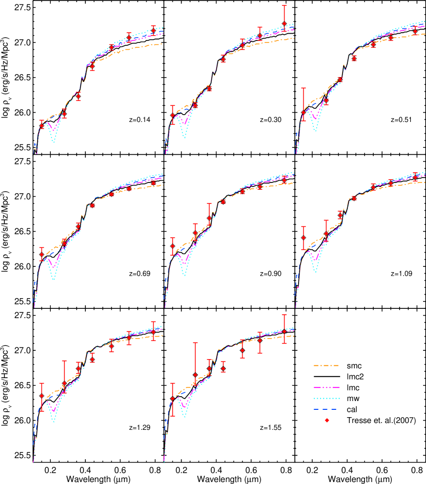
Figure 4.— The average comoving galaxy emissivity, $\rho_{\nu}$, at different $z$ calculated using our best fit combination of the SFRD($z$) and $A_{\rm FUV}(z)$ obtained for different models (with median $\rho_{\rm FUV}$ fits).The red diamonds are the $\rho_{\nu}$ measurements from Tresse et al. (2007). (See Fig. 17 in Appendix for $\rho_{\nu}$($z$) obtained for the low and high models at different wavebands along with the compiled luminosity density measurements.)

Figure 5.— The FUV band comoving luminosity density with $z$. Solid, dashed and dotted lines represent $\rho_{\nu}$ calculated at the FUV band using the median, high and low ‘lmc2’ model, respectively. The plotting symbols and corresponding references are mentioned in Table 1 for the FUV band. The $\rho_{\rm FUV}$ calculated for different models have negligible difference with respect to each other. Therefore, as a representative for all other models, we show $\rho_{\rm FUV}$ only for the ‘lmc2’ model.

In Fig. 4, we plot the $\rho_{\nu}$ obtained using convolution integral (Eq.7) for the best fit combinations of SFRD and $A_{\rm FUV}$ at different $z$ along with the measurements of Tresse et al. (2007). Note that, to get the $A_{\rm FUV}$ by least square minimization we use the $\rho_{\nu}$ measurements of Tresse et al. (2007) in all wavebands except at the FUV band. However, these $\rho_{\rm FUV}$ measurements along with many other reported in the literature up to $z=8$ (see Table 1 and Table 5) goes into fitting the $\rho_{\rm FUV}$ (as shown in Fig. 1). All our five models show very a good agreement with the measurements of Tresse et al. (2007) in all wavebands (including the FUV band). The difference in the strength of 2175Å absorption feature arises because of using different extinction curves.

In Fig. 5, along with the compiled measurements, we plot the $\rho_{\nu}$ at the FUV band obtained by using the combination of the SFRD$(z)$ and the $A_{\text{FUV}}(z)$ for the low, median and high ‘lmc2’ model. There are negligible differences in the $\rho_{\rm FUV}$ obtained for different models. Therefore, for clarity, we do not show the similar $\rho_{\rm FUV}$ plots for other models.

For the high $z$ and all other wavebands, we show our estimated $\rho_{\nu}$ along with the compiled measurements in Fig. 17 in the appendix (see Table 1 for the references and plotting symbols). Even though we use measurements of $\rho_{\nu}$ up to $z\sim 2$ and up to wavelength corresponding to the I band to get the $A_{\rm FUV}(z)$, our estimated $\rho_{\nu}$ matches well with various measurements up to $z\sim 4$ from the NUV to K band. This implies that our determined combinations of the $A_{\rm FUV}(z)$ and the SFRD($z$) are valid over a large $z$ range and suggests that our assumption of decreasing dust attenuation at high $z$ is also valid. However, note that, at the high redshifts (i.e, $z>4$) there are no measurements of $\rho_{\nu}$ except at the FUV band. In the H band, our calculated $\rho_{\nu}$($z$) is slightly over-estimated than the measured ones. However, as there are very few measurements we do not attempt to address this disagreement.

The good matching between the observations and the model predictions suggests that we have a consistent combination of the $A_{\rm FUV}(z)$ and SFRD($z$) for each extinction curve under consideration. The evolution of our best fit $A_{\rm FUV}$ and the corresponding SFRD with $z$ is discussed in the next section.

4.2. Redshift evolution of $A_{\text{FUV}}$

Understanding the dust attenuation and its wavelength and redshift dependences are very important to derive the intrinsic SFRD($z$) accurately. Dust attenuation is measured by using either of the SED fitting techniques, the Balmer decrement method or by comparing the FUV and the IR luminosity function measurements. It has also been noticed that at any given $z$, the derived $A_{\text{FUV}}$ may also depend on the galaxy luminosity and the stellar mass of the galaxy (see for e.g., Bouwens et al., 2012). Recently it has been shown that the shape of the extinction curve strongly depends on the distribution of the dust in the galaxies and the viewing geometries where scattering plays an important role (Chevallard et al., 2013). As our main purpose is to calculate the EBL, we are mainly interested in the volume averaged star formation rates and emissivity. Therefore, to calculate the average dust correction as a function of $z$, for simplicity we do not consider the dependence of $A_{\text{FUV}}$ on galaxy luminosity or stellar mass and the dependence of $k_{\nu}$ on scattering and viewing geometries. In this section, we compare the $A_{\text{FUV}}(z)$ obtained for different extinction curves with the $A_{\text{FUV}}$ measurements in the literature based on other independent approaches.

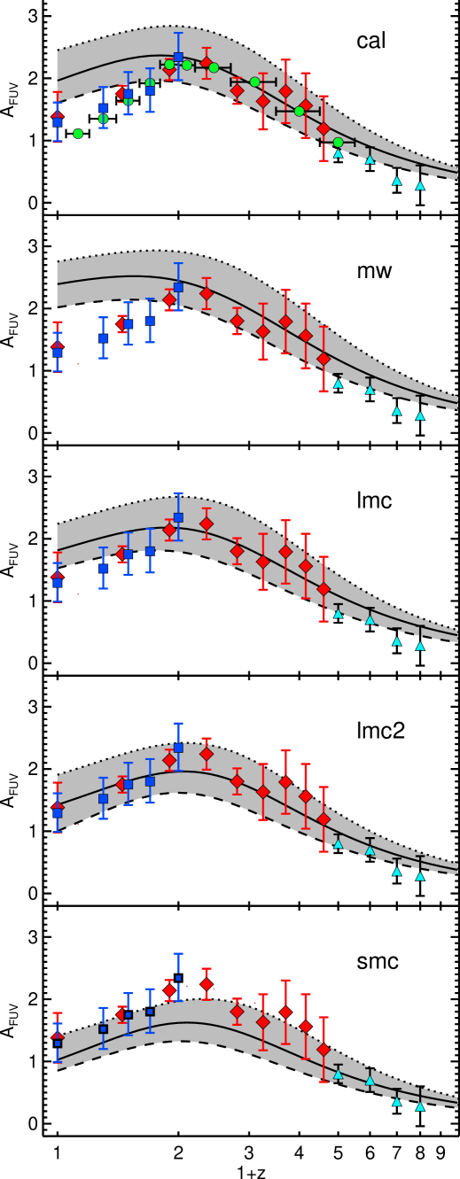
Figure 6.— Our best fit dust attenuation, $A_{\rm FUV}$, in magnitude as a function of redshift calculated by using different extinction curves. Dotted, solid and dashed lines represent values of the best fit $A_{\rm FUV}$ obtained using the low, median and high models, respectively. Green circles represent the A_FUV determined through the SED fitting by Cucciati et al. (2012) using Calzetti extinction curves. Red diamonds and Blue squares represents the A_FUV measured through $\rho_{\text{FIR}}$ to $\rho_{\text{FUV}}$ ratio by Burgarella et al. (2013) and Takeuchi et al. (2005), respectively. Cyan triangles are from Bouwens et al. (2012).

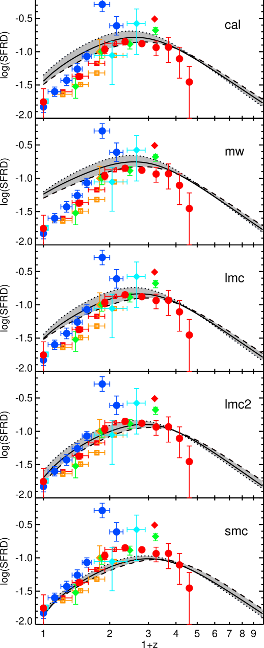
Figure 7.— Our best fit SFRD($z$) in units M_⊙ yr^-1 Mpc^-3 obtained using different extinction curves. Dotted, solid and dashed lines represent values of best fit SFRD($z$) obtained using the low, median and high models, respectively. Here, squares, diamonds and circles represent the SFRD($z$) determined from the radio, the H-$\alpha$ and the FIR observations, respectively. References and plotting symbols used here are provided in Table 3. The SFRD($z$) obtained using the LMC2 extinction curve shows good agreement with the different dust independent measurements.

Table 2Fitting parameters for the $A_{\rm FUV}$^∗

Extinction curve	$\rho_{FUV}$ fit†	a	b	c	d
SMC	Low	1.41	0.79	2.51	2.32
	Median	1.03	1.01	1.87	2.16
	High	0.85	0.86	1.77	2.16
LMC2	Low	1.91	0.85	2.40	2.23
	Median	1.42	0.93	2.08	2.20
	High	1.00	1.16	1.66	2.14
LMC	Low	2.24	0.79	2.51	2.21
	Median	1.81	0.82	2.12	2.06
	High	1.53	0.73	1.93	2.05
Milky-Way	Low	2.76	0.44	2.98	2.14
	Median	2.39	0.48	2.44	1.97
	High	2.02	0.49	2.15	1.97
Calzetti	Low	2.45	0.79	2.48	2.15
	Median	1.96	1.00	1.94	2.02
	High	1.61	0.91	1.81	2.03

*The fitting form is $A_{\rm FUV}(z)=\frac{a+bz}{1+(z/c)^{d}}$.
^†Note that, the models with low (high) $\rho_{\rm FUV}$ fit give higher (lower) A_FUV than the median model as explained in the text.

The fitting parameters for $A_{\text{FUV}}(z)$ for different extinction curves are given in Table 2. In Fig. 6, we plot the range of $A_{\text{FUV}}(z)$ for different extinction curves along with the measurements of Takeuchi et al. (2005), Cucciati et al. (2012), Burgarella et al. (2013) and Bouwens et al. (2012). Takeuchi et al. (2005) and Burgarella et al. (2013) determined the $A_{\text{FUV}}$ using the ratio of the FUV to FIR band luminosity density. Cucciati et al. (2012) have calculated the $A_{\rm FUV}$ using the Calzetti et al. (2000) extinction curve and used the SED fitting technique. At very high redshifts Bouwens et al. (2012) determined the effective dust extinction using the UV-continuum slope $\beta$ distribution and the IRX-$\beta$ relationship (see, Meurer et al., 1999). We take the effective extinction calculated for the luminosity function integrated up to -17.7 magnitude from Bouwens et al. (2012) (from table 6 of their paper).

The shaded region in Fig. 6 is obtained by using the low, high and median $\rho_{\rm FUV}$ fits to determine the $A_{\rm FUV}$. Since the SFRD is directly related to the $\rho_{\rm FUV}$ and $A_{\rm FUV}$, when we use the low (high) $\rho_{\rm FUV}$ fits, to get the same $\rho_{\nu}$ at different wavebands we need higher (lower) SFRD and hence higher (lower) $A_{\rm FUV}$. In other words, the low (high) $\rho_{\rm FUV}$ implies that the galaxies are more red (blue) which suggest that these galaxies should have more (less) dust extinction. This trend is evident from Fig. 6, where the dotted and dashed curves show the $A_{\rm FUV}$ obtained using the low and the high $\rho_{\rm FUV}$ fits, respectively.

The shaded region in Fig. 6 represents the allowed range of $A_{\rm FUV}$. For each assumed extinction curve, we get a different allowed range for the $A_{\rm FUV}$ and the difference is prominent at redshifts $z<1$. For redshifts $1<z<2$, we find that the $A_{\rm FUV}$ values remain constant or show a mild decrease with increase in $z$. At high redshifts, i.e $z>2$, our assumption of decreasing dust attenuation plays a role in getting similar allowed range of the $A_{\rm FUV}$ for all assumed extinction curves. As can be seen from Fig. 6, the allowed $A_{\rm FUV}$ range for $z>2$ nicely follows that of other independent measurements rendering support to our assumption. Apart from the $A_{\rm FUV}$ determined for the ‘mw’ model, for all the other models we find a moderate increase in the $A_{\rm FUV}$ with redshift up to $z=1$ from $z=0$. This trend of increasing FUV band dust attenuation magnitude has been detected previously (see, Takeuchi et al., 2005; Cucciati et al., 2012; Burgarella et al., 2013) as shown in Fig. 6. However, at $z\leq 0.8$, our estimated $A_{\text{FUV}}(z)$ for ‘cal’, ‘mw’, and ‘lmc’ models are higher than these measurements. The $A_{\rm FUV}$ determined for ‘smc’ model matches well in all redshifts expect that it under-predicts $A_{\rm FUV}$ at $1<z<2$. Overall, a good match with these measurements of the $A_{\rm FUV}$ is obtained over the large $z$ range for the ‘lmc2’ model.

From the very good agreement between the $A_{\rm FUV}(z)$ determined for the ‘lmc2’ model and the measurements of Burgarella et al. (2013) and Takeuchi et al. (2005), we conclude that the average extinction curve which is applicable for galaxies over wide range of redshifts is most likely to be similar to LMC2 extinction curve.

Recently, Kriek & Conroy (2013) using SED of the galaxies investigated the dust extinction curves for 32 different spectral classes of galaxies over $0.5\leq z\leq 2$. They found that the Milky-Way and Calzetti extinction curves provide poor fits to the UV wavelengths for all SEDs. They concluded that the SED with the $2175\AA$ UV bump albeit weaker in strength compared to the Milky-Way is preferred. Buat et al. (2012) studied a sample of 751 galaxies with redshift $0.95<z<2.2$ and found that the mean parameters describing the dust attenuation curves are similar to those found for the LMC2 extinction curve. This is consistent with what we find here. It is interesting to note that in the case of intervening absorption systems seen in the QSO spectra, the high percentages of systems with the $2175\AA$ absorption feature detection favors the LMC2 extinction curve (see for e.g. Srianand et al., 2008; Noterdaeme et al., 2009; Jiang et al., 2013). It has also been observed that the extinction curves for individual galaxies depend on the type and other galaxy properties (Wild et al., 2011; Chevallard et al., 2013; Kriek & Conroy, 2013). Therefore, single universal extinction curve for all galaxies may not be realistic. However, our study suggests that for estimating the volume average properties like the SFRD, $A_{\rm FUV}$ and EBL the LMC2 extinction curve should be preferred.

4.3. Redshift evolution of SFRD

We assume that the SFRD is a smooth and continuous function of $z$ and fit it with the same functional form (using Eq. 9) we are using to fit the $\rho_{\rm FUV}$ and $A_{\rm FUV}$. The fitting parameters for the SFRD$(z)$ are given in Table 4. In Fig. 7, we plot the SFRD($z$) for all the five extinction curves with their high and low models. As explained earlier we get the high (low) SFRD for low (high) $\rho_{\rm FUV}$ fits. Since the SFRD is directly proportional to the $\rho_{\rm FUV}$ and $A_{\rm FUV}$, at $z>3$, where differences in the $A_{\rm FUV}$ for all high and low models are small, the term $\rho_{\rm FUV}$ dominates and the SFRD($z$) curves cross each other as demonstrated in Fig. 7.

Table 3SFRD from different observations

Reference	Technique	Redshift range	Plotting Symbols
Shim et al. (2009)	H-$\alpha$	0.7-1.9	cyan diamond
Tadaki et al. (2011)	H-$\alpha$	2.2	red diamond
Sobral et al. (2013)	H-$\alpha$	0.4-2.3	green diamond
Ly et al. (2011)	H-$\alpha$	0.8	orange diamond
Condon et al. (2002)	1.4 GHz	0.02	cyan squares
Smolčić et al. (2009)	1.4 GHz	0.1-1.3	red & orange squares
Rujopakarn et al. (2010)	FIR	0-1.3	blue circles
Burgarella et al. (2013)	FIR	0-4	red circles

In Fig. 7, we also plot the SFRD determined through different observations.There are different indicators of star formation but not all are independent of the assumed dust correction. Therefore for comparison we use the SFRDs determined through the radio, H-$\alpha$ and FIR emission from galaxies. We do not consider the SFRD determined with observations like the UV luminosity where it mainly depends on the assumed values of $A_{\rm FUV}$ and the extinction curve. We select the measurements where luminosity densities are converted to the SFRD using conversion laws (see Eq. 6) with assumed Salpeter IMF with stellar mass with range 0.1 to 100 M_⊙, similar to the one we use. Table 3 summarizes the references to such a data and indicates the plotting symbols used for it in Fig. 7. Our inferred SFRD($z$) using the ‘cal’, ‘lmc’ and ‘mw’ models are higher than these SFRD measurements with different techniques at $z<1$ (see, Fig. 7). The SFRD($z$) calculated for the ‘smc’ model is consistent with SFRD measurements using radio observations at low $z$ but under-predict the SFRD at $2>z>1$. We find that the SFRD($z$) determined using the ‘lmc2’ model fits th e SFRD data well at all $z$. Like in the case of $A_{\rm FUV}$, determination of SFRD$(z)$ based on the LMC2 extinction curve provides the best fit to the different independent measurements compared to those of other models.

From Fig. 6 and Fig. 7, it is clear that, irrespective of the extinction law used, we find the $z$ at which the SFRD($z$) peaks is higher than the $z$ beyond which $A_{\rm FUV}$($z$) begins to decline. The similar trend in peaks of SFRD and $A_{\rm FUV}$ has reported in Cucciati et al. (2012) and Burgarella et al. (2013).

Figure 8.— Our best fit SFRD($z$) in units M_⊙ yr^-1 Mpc^-3 obtained using the LMC2 extinction curve. The gray shaded region gives the range covered by the low and high models. We also plot the SFRD($z$) determined by Madau & Dickinson (2014) using measurements of $\rho_{\rm FUV}$ for the same IMF we use but with different metallicity. To compare the general trend, we also plot the SFRD($z$) fit given by Behroozi et al. (2013) for the different observational determination of the SFRD given in literature for the recent data and the old data compiled by Hopkins & Beacom (2006). Both these fits are for Chabrier (2003) IMF. We scaled the Hopkins & Beacom (2006) fit by 2.5 for clarity.

In Fig. 8 we plot our SFRD obtained using the LMC2 extinction curve along with the SFRD determined by Madau & Dickinson (2014). Shaded region in Fig. 8 represents SFRD range covered when we use low and high ‘lmc2’ models to determine the SFRD and $A_{\rm FUV}$. Madau & Dickinson (2014) used the $\rho_{\rm FUV}$ measurements from the literature and converted them in to the SFRD using the conversion constant $\zeta=1.15\times 10^{-28}$ which is 10% smaller than what we use. For the dust correction they use the $A_{\nu}$ provided by the different surveys from where the luminosity functions are used to get the $\rho_{\rm FUV}$. They calculate the $\rho_{\rm FUV}$ by integrating the luminosity function from $L_{min}=0.03L^{*}$, while in our case we directly take $\rho_{\rm FUV}$ given in different references where it is often calculated with $L_{min}=0$ (for the $L_{min}$ values used here, see Table 5 in appendix). Madau & Dickinson (2014) use the same IMF used by us but take different metallicities and consider metallicity evolution with $z$. As compared to our preferred SFRD($z$) for the LMC2 model the SFRD of Madau & Dickinson (2014) shows rapid increase and decrease in low and high $z$, respectively. However, the difference between both is within 0.1 to 0.2 dex for $z<5$. The peak of SFRD($z$) of our preferred ‘lmc2’ model matches exactly with that of Madau & Dickinson (2014). The peak of our SFRD($z$) is at $z=1.9^{+0.2}_{-0.3}$ which is also consistent with the peak of SFRD reported by Cucciati et al. (2012).

Table 4Fitting parameters for the SFRD($z$)^∗

Extinction	$\rho_{FUV}$	a	b	c	d
curve	fit†	(10-2)	(10-2)
SMC	Low	1.55	7.14	2.53	3.10
	Median	1.38	6.24	2.65	3.01
	High	1.50	5.12	3.08	3.09
LMC2	Low	2.54	10.9	2.22	3.07
	Median	2.01	8.48	2.50	3.09
	High	1.67	7.09	2.74	3.02
LMC	Low	3.57	13.6	2.15	3.13
	Median	3.13	9.88	2.37	3.03
	High	3.03	7.37	2.70	3.01
Milky-Way	Low	6.27	15.2	2.14	3.16
	Median	5.78	11.2	2.28	3.02
	High	5.03	8.33	2.59	2.99
Calzetti	Low	4.44	15.8	2.06	3.11
	Median	3.62	12.0	2.20	2.97
	High	3.23	8.78	2.54	2.97

*The fitting form is ${\rm SFRD}(z)=\frac{a+bz}{1+(z/c)^{d}}$ M_⊙ yr^-1 Mpc^-3 .
^†Note that, as explained in the text, the models with low and high $\rho_{\rm FUV}$ fit need not to give higher and lower SFRD($z$) than median model for all $z$, respectively.

For comparing the SFRD($z$) shapes, we also plot the fit to the SFRD measurements compiled from the different observational data reported in the literature given by Behroozi et al. (2013) (see figure 2 and table 4 of their paper). Behroozi et al. (2013) provides the fit for the recent data and the old data used by Hopkins & Beacom (2006). Both of these fits are obtained for Chabrier (2003) IMF and show rapid increase at low $z$ as compared to our SFRD($z$). At high $z$, the fit through compiled SFRD data used by Hopkins & Beacom (2006) shows the slow decrease while Behroozi et al. (2013) fit shows rapid decrease as compared to our SFRD. The peak of the compiled SFRD measurements of Behroozi et al. (2013) for the old and new measurements is at $z=1.7$ which is consistent with our SFRD$(z)$ peak within the allowed uncertainties. The main differences between our SFRD$(z)$ estimated here and the compiled SFRD measurements of Behroozi et al. (2013) and SFRD($z$) estimated by Madau & Dickinson (2014) is that we self-consistently calculate the $A_{\rm FUV}(z)$ which gives SFRD$(z)$ consistent with $\rho_{\nu}$ measurements at different wavebands and redshifts.

Having obtained the best fit $A_{\rm FUV}$($z$) and SFRD($z$), we use the stellar population synthesis models to calculate the emissivity from UV to NIR regime. However, to generate the complete EBL, in addition to this we need the IR emissivity. We predict the IR emissivity using our best fit $A_{\rm FUV}$($z$) and SFRD($z$) which is explained in the following section.

5. Galaxy emissivity in infrared

The old stellar population, the interstellar gas and the dust are main sources which contribute to the IR emission form galaxies. The IR emission from old stars peaks around 1 to 3$\mu$m and a very few per cent of the total IR output of a galaxy is emitted by atoms and molecules that constitute the interstellar gas. The main source of the IR emission at $\lambda>3\mu$m is a thermal emission from the dust grains heated by the local stellar light in the UV and optical wavelength range. The amplitude and shape of this emission from the NIR to FIR wavelengths depend on the temperature, size distribution and the composition of the dust grains (e.g. Dale et al., 2012; Magdis et al., 2012, 2013). However, like the extinction curves, these quantities are unknown for distant galaxies. Therefore, instead of assuming the dust properties to model the NIR to FIR emission of a typical galaxy, we use the observed IR templates and make use of the $A_{\rm FUV}$ for different models determined here.

We use the average IR templates of Rieke et al. (2009) from 5$\mu$m to $30$cm obtained for infrared galaxies having different total infrared luminosity, $L_{\rm TIR}$. They have assembled the SEDs of 11 local luminous and ultra-luminous infrared galaxies and for generating the templates at lower luminosity they have combined the templates of Dale et al. (2007) and Smith et al. (2007). The shape of each template is moderately different for different $L_{\rm TIR}$. Therefore, we have to choose an appropriate template for calculating the IR emission. Since at any $z$, most of the total luminosity is contributed by the galaxies with luminosity $L^{*}(z)$, we choose templates of Rieke et al. (2009) obtained for $L_{\rm TIR}=L_{\rm TIR}^{*}(z)$. We use $L_{\rm TIR}^{*}(z)$ values for different redshift using the total IR luminosity function given in Gruppioni et al. (2013) up to $z=4$. To get the $L_{\rm TIR}^{*}(z)$ values for the high redshifts (in units $L_{\odot}$) we fit a second degree polynomial through $log(L_{\rm TIR}^{*})$ using mpfit IDL routine. The best fit second degree polynomial is $log[L_{\rm TIR}^{*}(z)]=10.0+1.18z-0.18z^{2}$. To compute the FIR spectrum we interpolate the templates of Rieke et al. (2009) for corresponding values of $L_{\rm TIR}^{*}(z)$ given by the above polynomial fit. For all redshifts $z>7$ we use the interpolated template of Rieke et al. (2009) with $L_{\rm TIR}^{*}=10^{9}L_{\odot}$. However this lower limit has no effect on the shape of IR template since it is just a template for lowest luminosity ($10^{9.75}L_{\odot}$) given by Rieke et al. (2009) scaled to give the $L_{\rm TIR}=10^{9}L_{\odot}$.

We use the energy conservation to calculate the IR emission. We assume that the average energy absorbed by the dust from FUV to NIR regime per Mpc³ per $s$ at any redshift $z_{0}$, $E_{abs}(z_{0})$, is emitted in the NIR to FIR regime as a thermal emission with the assumed SED taken from the appropriate IR template at $z_{0}$ as explained above. The $E_{abs}(z_{0})$ is given by,

$$E_{abs}(z_{0})=\int_{\nu_{i}}^{\nu_{f}}d\nu\Big{[}1-C_{\nu}(z_{0})\int_{z_{0}}^{\infty}{\rm SFRD}(z)\,\,l_{\nu}(t_{0}(z),Z)\,\,dz\,\Big{]},$$ (11)

where, $C_{\nu}(z_{0})=10^{-0.4\,A_{\nu}(z_{0})}$ and $\nu_{i}$ and $\nu_{f}$ are the frequencies corresponding to 0.092$\mu$m and 10$\mu$m. Photons in this wavelength range heat the interstellar dust effectively. Hard photons at $\lambda<0.092\mu$m are mainly photo-absorbed by the interstellar hydrogen and helium. We assume that $E_{abs}(z_{0})$ is emitted at the same time in IR from 5 to 1000$\mu$m. We scale the IR template with total IR luminosity $L_{\rm TIR}^{*}(z_{0})$ to match the value of $E_{abs}(z_{0})$ in between wavelength from 5 to 1000$\mu$m. Then we do a power law extrapolation to this scaled IR template at $\lambda<5\mu$m. We use a second degree polynomial to smoothly connect the NIR part of the SED with the IR part of the extrapolated template at the connecting points. Note that, here we assume the efficiency of dust to re-emit in the NIR to FIR wavelengths is 100%.

Figure 9.— The galaxy emissivity at $z=0$ for different models. Apart from the $2175$Å absorption feature, in the IR ($\lambda>1\mu$m) the difference between different models can be easily seen. The data in the optical and NIR ($0.35\leq\lambda<3\mu$m) is taken from Montero-Dorta & Prada (2009) and Jones et al. (2006). Emissivity measurements in the NIR to FIR wavelengths ($8\leq\lambda\leq 850\mu$m) are taken from Huang et al. (2007), Soifer & Neugebauer (1991), Takeuchi et al. (2006) and Serjeant & Harrison (2005)

In Fig. 9, we show the emissivity of galaxies from the UV to FIR at $z=0$ for the different extinction curves assumed. As expected, apart from the $2175\rm\AA$ absorption feature the emissivity up to $\lambda=0.8\mu$m is quite same for all models. However, from the NIR to FIR wavelengths the emissivity is different for different models. This is because the absorbed energy by the interstellar dust depends on the extinction curve and the $A_{\rm FUV}$. In Fig. 9, we also show the local emissivity from different surveys and at different wavelengths like in the optical from SDSS by Montero-Dorta & Prada (2009), in the NIR wavelength from the 2MASS and 6dF by Jones et al. (2006), in the IR to FIR from surveys like ISO FIRBACK, IRAS and SCUBA by Soifer & Neugebauer (1991), Takeuchi et al. (2006) and Serjeant & Harrison (2005) and at 8$\mu$m from Spitzer space telescope survey by Huang et al. (2007). Our predicted local emissivity from the NIR to FIR ($\lambda>2\mu$m) range in case of the ‘mw’ and ‘cal’ models give higher intensity by factor $\sim 2$ than the local emissivity measurements from these different surveys. Our local emissivity for the ‘lmc’ and ‘smc’ models are marginally higher and lower from these measurements, respectively. Our ‘lmc2’ model gives a local emissivity which is in very good agreement with these measurements.

In principle, the dust can be assumed to have lower efficiency to re-emit. In that case, the models which give higher IR emissivity can be scaled down to reproduce the measurements. But there is no room for scaling up the IR emission form the models which give lower IR emissivity. Therefore, the ‘smc’ model can not be scaled up to match the local emissivity measurements.

We use the emissivity of galaxies from UV to FIR range obtained here to calculate the EBL which is discussed in detail in the following section.

6. EBL Calculation

We solve the cosmological radiative transfer equation (Eq. 2) numerically to compute the EBL. In this equation the source term, $\epsilon_{\nu}$, is the sum of the QSO and galaxy emissivities. We take the QSO emissivity, $\epsilon_{\nu,\rm Q}(z)$, and the SED as given in Section 2. We use the galaxy emissivity from the combinations of the SFRD($z$) and A${}_{\rm FUV}(z)$ for different dust extinction curves and corresponding dust emission as described in the previous sections. In the following sections, we compare our estimated EBL from UV to FIR regime with the direct measurements of the local EBL and other estimates of the EBL reported in the literature.

6.1. The local EBL

First, we compute the EBL at $z=0$ for our five different models which are plotted in Fig. 10. Apart from the wavelengths near the 2175Å absorption, different EBLs are quite indistinguishable from each other for $\lambda<0.8\mu$m. As expected, we see a clear differences appearing at higher wavelengths between different models. Apart from the extinction curves, the difference is also because of the differences in $A_{\rm FUV}$ values for the different models (see Fig. 6). Therefore, even though the estimated EBL in the UV and optical parts are similar (because of the way we determine SFRD and $A_{\rm FUV}$), there are clear differences in the IR wavelengths where the dust re-emission is important.

Figure 10.— The EBL at $z=0$ for different models. The shaded region represents the range of the allowed EBL intensity from observations. The lower limits are determined by the intensity of the IGL (squares). While the upper limits are determined by the direct measurements of the EBL (circles). The data used here is taken from Dwek & Krennrich (2013) and references their in. The IR predictions of the ‘smc’ model are inconsistent with the observations. The stars are the sum of the IGL background compiled by Franceschini et al. (2008) and the estimated intra-halo light from the measured fluctuations of EBL by Zemcov et al. (2014).

The shaded area in Fig. 10 represents the range of the allowed EBL intensity determined by the local EBL observations. The data used in Fig. 10 is taken from compilation of Dwek & Krennrich (2013) (see their Fig. 7). The lower limits are determined by the intensity of integrated galaxy light (IGL). The IGL is obtained by adding the light emitted by resolved galaxies in deep surveys. In principle the IGL should converge to the total EBL at $z=0$. However, because of the problem in the convergence of number counts and sensitivity of the surveys to resolve fainter galaxies, the IGL gives a lower limit to the EBL. Here, we use the IGL measurements in the UV from Galex (Galaxy Evolution Explorer), in the optical from HST and in the IR from Spitzer, ISO and Herschel (Totani et al., 2001; Xu et al., 2005; Levenson et al., 2007; Fazio et al., 2004; Béthermin et al., 2010; Berta et al., 2010). The upper limits on the local EBL come from the direct measurements of the EBL. Important uncertainty in the direct measurements is the removal of strong foreground zodiacal light caused by the interplanetary dust and the stellar emission from the Milky-way. Therefore, these measurements provide a strict upper limits on the local EBL. In Fig. 10, we take the absolute measurements of EBL in the optical from Pioneer 10/11 and in the IR from COBE (Fixsen et al., 1998; Dwek & Arendt, 1998; Finkbeiner et al., 2000; Dole et al., 2006; Levenson et al., 2007; Matsuoka et al., 2011; Matsuura et al., 2011).

Our EBL estimate for the ‘smc’ model goes below the lower limits at $\lambda>1\mu$m. While for all other models, the estimated EBL is within the allowed range. If we strictly follow the shaded region, we can rule out the ‘smc’ model and conclude that the average extinction curve for galaxies is inconsistent with the SMC type of dust extinction. However, the allowed range is too large to distinguish between other models. All our EBL models in the UV, optical and NIR ($\lambda<2\mu$m) follow the lower limits of the EBL where we use the emissivity consistent with the observed multi-wavelength galaxy luminosity functions. The ‘lmc2’ model, which also provides the $A_{\rm FUV}(z)$ and SFRD$(z)$ consistent with different independent measurements, produces the IR background ($1<\lambda<100\mu$m) consistent with the lower limits while other models produce slightly higher background intensity but well within the allowed range and closer to the lower limits. In the FIR regime ($\lambda>100\mu$m), the estimated background for the ‘lmc2’ and ‘lmc’ model goes through the observed points. The EBL for the ‘mw’ and ‘cal’ models are just consistent or slightly higher than the observed upper limits at $\lambda>100\mu$m. In summary, the available local EBL measurements in the NIR to FIR regime doest not support the average dust extinction similar to the one observed in case of SMC. However, these measurements can not discriminate between the EBL obtained with other extinction curves.

Recently, using the rocket-borne instrument Cosmic Infrared Background Experiment (CIBER), Zemcov et al. (2014) have measured the fluctuation amplitude of IR background at $1.1\mu$m and $3.6\mu$m. One of the plausible explanations for the large fluctuation found at these wavelengths is that it arises from the intra-halo light (IHL) produced by the tidally striped old stars in the halo of the galaxy (Cooray et al., 2004; Thacker et al., 2014). Using these fluctuations measured over the large scales Zemcov et al. (2014) gives the model dependent total EBL contributed by IHL. In Fig. 10, we show their computed values of the total EBL which is sum of their estimated IHL and the compiled measurements of IGL by Franceschini et al. (2008). As expected, since we do not include the additional contributions like the IHL in our emissivities, we find that our estimated EBL for all models is lower than the predicted by Zemcov et al. (2014). Except for the ‘smc’ model, the EBL obtained for all other models at $\lambda\leq 2.4\mu$m are within 2-$\sigma$ lower than the total EBL predicted by Zemcov et al. (2014). We find that only for the ‘smc’ model it is more than 2.5-$\sigma$ lower at all wavelengths. At $\lambda\geq 3.6\mu$m our ‘lmc’, ‘mw’ and ‘cal’ models match with the EBL predicted by Zemcov et al. (2014) within 1-$\sigma$. In the light of these recent developments, it will be interesting to consider the IHL contribution to IR, the signal arising from the epoch of re-ionization (Cooray et al., 2004; Kashlinsky et al., 2004) and the FIR light from dusty galaxies (Amblard et al., 2010; Thacker et al., 2013; Viero et al., 2013) which we will attempt in the near future.

From the very good agreement with the local emissivity (see Fig. 9) and with different independent measurements of the $A_{\rm FUV}(z)$ and SFRD$(z)$ (see Fig. 6 and 7), for the EBL calculations we prefer our ‘lmc2’ model over other models.

6.2. High $z$ EBL

In Fig. 11, we plot the EBL at redshifts 0, 0.5, 1 and 1.5 for our preferred ‘lmc2’ model. We also show the range covered by the high and low ‘lmc2’ model by a gray shaded region and the range covered by all five median models by a vertical striped region. The fact that we made sure the SFRD($z$) and A${}_{\rm FUV}(z)$ determined for different extinction curves should give the same observed emissivity has resulted in the narrow spread in the striped region for $\lambda<3\mu$m, especially at high redshifts. For comparison, in Fig. 11, we also show the previous estimates of the EBL reported in the literature (Inoue et al., 2013; Gilmore et al., 2012; Finke et al., 2010; Kneiske & Dole, 2010; Franceschini et al., 2008; Domínguez et al., 2011; Helgason & Kashlinsky, 2012; Scully et al., 2014, HM12). Below we compare our EBL predictions with the previous EBL estimates which use observational data like galaxy number counts and galaxy luminosity functions to get the EBL directly.

Figure 11.— The predicted EBL at different redshifts for our preferred ‘lmc2’ model. The gray shaded region shows the EBL covered by the high and low ‘lmc2’ model. The vertical striped region gives the range covered by all other median models with different extinction curves. For comparison we plot other estimates of the EBL from literature. In the top left panel the yellow diamonds are the lower limit data compiled by Kneiske & Dole (2010). For clarity the legends are distributed over the entire plot. Note that the EBLs presented here are in proper units.

Helgason & Kashlinsky (2012) and (Stecker et al., 2012) reconstructed the EBL using the multi-wavelength and multi-epoch luminosity functions. We also use a similar compilation of luminosity functions but up to the $K$ band. Therefore, our EBL matches very well with the EBL predictions of Helgason & Kashlinsky (2012) up to $\lambda\sim 3\mu$m, as shown in Fig. 11. For $\lambda>3\mu$m, Helgason & Kashlinsky (2012) predicts the higher EBL intensity than us. The EBL model of (Scully et al., 2014) extend the model of (Stecker et al., 2012) upto 5$\mu$m and provide 1-$\sigma$ upper and lower limits on the EBL as well as $\tau_{\gamma}$. Our EBL predictions are consistent with their lower and upper limit EBL for $\lambda>1\mu$m. The EBL estimated by Domínguez et al. (2011) is based on the observed K-band luminosity function with the galaxy SEDs based on the multi-wavelength observations from the SWIRE library. For $z<1$ and $\lambda\sim 3\mu$m, our EBL is consistent with the predictions of Domínguez et al. (2011) which shows slightly lower EBL intensities in the UV and slightly higher EBL intensities in the NIR. At high $z$ this difference is more prominent. Franceschini et al. (2008) used different multi-wavelength survey data which includes luminosity functions, number counts and the redshift distribution of different galaxy types and the relevant data is fitted and interpolated to get the EBL. Our estimated EBL matches well with the EBL of Franceschini et al. (2008) up to NIR wavelengths. At $z>1$, in the UV regime their EBL gives factor $\sim 1.5$ lower intensity than our EBL. However in the FIR wavelengths, our EBL gives around factor $\sim~{}2$ smaller EBL intensity as compared to the EBL of Franceschini et al. (2008) and Domínguez et al. (2011). In summary, as expected our EBL at $\lambda<3\mu$m is consistent with the models which use direct observations to get the EBL but gives a lower EBL in the NIR to FIR regime. Below we mention some of the general trends in different EBL estimates that can be seen from Fig. 11.

Given that there are more observations of the EBL as well as the luminosity functions of galaxies in the local Universe, almost all the different independent models including our ‘lmc2’ model converge very well, spans narrower range at $z=0$ in the UV to NIR regime and pass through observed lower limits of EBL. However, at the NIR and FIR wavelengths the spread between different estimates is relatively higher. All the EBL estimates differ from each other at high $z$ and the difference is as high as factor $\sim$4. Our local EBL passes very well through the lower limit EBL data compiled by Kneiske & Dole (2010). Most of the EBL models for $0.4<\lambda<2\mu$m give similar intensity upto $z<1.5$.

Our local EBL is very much similar to the estimates of HM12. However, at higher $z$, the UV background ($\lambda<0.4\mu$m) intensity of HM12 is higher than our EBL. This will have implications on the values of escape fraction for H i ionizing photons which indirectly plays an important role in interpreting He ii Lyman-$\alpha$ effective optical depth measurements near the epoch of Helium reionization (see, Khaire & Srianand, 2013).

Having obtained the EBL at different $z$ from UV to FIR, we calculate its effect on the transmission of high energy $\gamma$-rays through the IGM and compare it with the different observations in the following section.

7. Gamma ray attenuation

Two photons with sufficient energy upon collision can annihilate into an electron positron pair. The condition on energies of photons ($E_{1}$ and $E_{2}$) for this process of pair production is given by

$$\sqrt{2E_{1}E_{2}(1-\cos\theta)}\geq 2m_{e}c^{2},$$ (12)

where, $\theta$ is the collision angle, $m_{e}$ is the mass of the electron and $c$ is the speed of light. Thus $\gamma$-rays with an energy $E_{\gamma}$ can annihilate themselves with the background extra-galactic photons having energy greater than a threshold energy $E_{th}$,

$$E_{th}=\frac{2m_{e}^{2}c^{4}}{E_{\gamma}(1-\cos\theta)}.$$ (13)

The cross-section for this process is,

$$\sigma(E_{1},E_{2},\theta)=\frac{3\sigma_{T}}{16}(1-\beta^{2})$$ (14)

$$\times\left[2\beta(\beta^{2}-2)+(3-\beta^{4})\ln\left(\frac{1+\beta}{1-\beta}\right)\right],$$

where,

$$\beta=\sqrt{1-\frac{2m_{e}^{2}c^{4}}{E_{1}E_{2}(1-\cos\theta)}}\,\,,$$

and $\sigma_{T}$ is the Thompson scattering cross-section. The pair production cross-section given in Eq. 14 has a maximum value $\sigma(E_{1},E_{2},\theta)_{max}=0.25\,\sigma_{T}$ and the corresponding value of $\beta=0.7$.

If the number density of background photons at redshift $z$ and energy $E_{bg}$ is $n(E_{bg},z)$ (from Eq. 1), then as a result of pair production the optical depth encountered by the $\gamma$-ray photons emitted at redshift $z_{0}$ and observed at energy $E_{\gamma}$ on the Earth (i.e. at $z=0$) is given by

$$\tau_{\gamma}(E_{\gamma},z_{0})=\frac{1}{2}\int^{z_{0}}_{0}dz\;\frac{dl}{dz}\int^{1}_{-1}d(\cos\theta)\;(1-\cos\theta)$$ (15)

$$\times\int^{\infty}_{E_{min}}dE_{bg}\;n(E_{bg},z)\;\sigma(E_{\gamma}(1+z),E_{bg},\theta).$$

Here,

$$E_{min}=E_{th}\>(1+z)^{-1}=\frac{2m_{e}^{2}c^{4}}{E_{\gamma}(1+z)(1-\cos\theta)}\,\,.$$ (16)

Above equation in terms of the maximum wavelength of the EBL, which is going to attenuate observed $\gamma$-rays of energy $E_{\gamma}$, can be simplified as $\lambda_{max}(z)=23.74\text{\AA}E_{\gamma}(1+z)(1-\cos\theta)$ where $E_{\gamma}$ is in GeV. The cross-section for the pair production will be maximum at $\lambda(z)=12.06\text{\AA}E_{\gamma}(1+z)(1-\cos\theta)$.

The specific number density of the EBL photons is directly related to the optical depth $\tau_{\gamma}$ encountered by $\gamma$-rays while traveling through the IGM as explained above. For the EBL estimated here, we calculate $\tau_{\gamma}$ using Eq. 15 over a energy range from GeV to TeV. In the following sub-section, we compare our calculated of $\tau_{\gamma}$ with those obtained using different EBL estimates reported in the literature.

Figure 12.— Top panel: The $\gamma$-ray optical depth, $\tau_{\gamma}$, for different emission redshifts for observed $\gamma$-ray energy using our preferred ‘lmc2’ EBL (red curve) along with the $\tau_{\gamma}$ from other EBL estimates from the literature. For clarity the legends are distributed over the entire plot. Dark gray shaded region gives the range covered in $\tau_{\gamma}$ by the high and low ‘lmc2’ EBL models. The light gray shaded region gives the range covered by all five of our EBL models. Bottom panel: The ratio of $\tau_{\gamma}$ predictions of different models to the $\tau_{\gamma}$ obtained for our ‘lmc2’ model.

7.1. The $\gamma$-ray opacity at different $z$

The optical depth encountered by $\gamma$-rays while traveling from the emission redshifts $z_{0}$ to earth (i.e, $z=0$) and observed at $\gamma$-ray energies from GeV to TeV range is plotted in Fig. 12 for different emission redshifts. We plot $\tau_{\gamma}$ calculated for our median ‘lmc2’ model along with the $\tau_{\gamma}$ for its low and high counterparts in a dark gray shaded region. We also show the range of $\tau_{\gamma}$ covered by all five median models by a light gray shaded region. The extent of the light gray shaded region for different $z$ up to the $\gamma$-ray energy of 0.6 TeV shows that the $\tau_{\gamma}$ is indistinguishable for all five EBL models. This is because the maximum effective wavelength of EBL photons which interact with $\gamma$-rays of energy less than 0.6 TeV is less than $3\,\,\mu$m where, by construct, our different EBL models predict similar intensities (see Fig. 11). The spread of shaded region for $\gamma$-ray energy $>$ 0.6 TeV points to the fact that our EBL intensity at FIR wavelengths is different for different models.

For comparison, in Fig. 12, we also plot the $\tau_{\gamma}$ obtained by other estimates of EBL given in the literature. To clearly show the differences between $\tau_{\gamma}$ calculated for other EBL estimates and for our ‘lmc2’ EBL model, we plot the ratio of the former to the later in the bottom panel of Fig. 12. Differences in the $\tau_{\gamma}$ obtained for various EBL estimates can be directly understood from the differences in the EBLs as shown in Fig. 11. Here, we mention some of the general trends seen in the various $\tau_{\gamma}$ estimates and then compare our $\tau_{\gamma}$ with the models which used direct observations of galaxy properties to construct the EBL.

The difference between the $\tau_{\gamma}$ at energies from GeV to TeV for various EBL estimates increases with $z$. The difference is more in the TeV energy range where the EBL photons which effectively attenuate the $\gamma$-rays are from the FIR part of the EBL. The large scatter in different EBL estimates in the FIR wavelengths (see, Fig. 11) is responsible for that. However, for the observationally relevant $\gamma$-rays which are the ones with $0.1<\tau_{\gamma}<2$ where in the corresponding energy range the differences between $\tau_{\gamma}$ estimates are quite small. The difference in $\tau_{\gamma}$ for $\gamma$-ray energies from 0.1 to 3 TeV is small and within 30% for various estimates for emission redshifts $z<1.5$. In general, our EBL gives lower $\tau_{\gamma}$ compared to most of the other estimates. The $\tau_{\gamma}$ obtained for lower limit EBL of Scully et al. (2014) at $z=0.01$ is factor $\sim 2$ higher at $E_{\gamma}<0.2$TeV. The $\tau_{\gamma}$ obtained for the EBL by Inoue et al. (2013) at $z\geq 1$ is within the 10% of our estimate at $0.2<E_{\gamma}<40$TeV. However, note that the $\tau_{\gamma}$ at $E_{\gamma}>10$ TeV in our model is quite small because we do not consider the CMBR in our EBL model (see Stecker et al., 2006). The $\tau_{\gamma}$ in the energy range $0.05<E_{\gamma}<2$ TeV estimated by Helgason & Kashlinsky (2012) upto $25\mu$m is within 15% of our $\tau_{\gamma}$. The $\tau_{\gamma}$ calculated using the EBL generated by Franceschini et al. (2008) and Domínguez et al. (2011) for $0.1<E_{\gamma}<4$ TeV is within the 30% of our $\tau_{\gamma}$. However, at high energies, $\tau_{\gamma}$ differs more than this which is evident from the differences in the FIR part of the EBL in between their models and our ‘lmc2’ model (see, Fig. 11).

Figure 13.— The $\gamma$-ray horizon plotted for different EBL models. Data points are from Domínguez et al. (2013). Gray area shows range covered by EBL in the high and low ‘lmc2’ models.

7.2. $\gamma$-ray horizon

The $\gamma$-ray horizon is defined as the maximum redshift of the $\gamma$-ray source that can be detected through $\gamma$-rays of observed energy $E_{\gamma}$ with $\tau_{\gamma}\leq 1$. This is nothing but the $\gamma$-ray source redshift $z_{0}$ for $\gamma$-rays of observed energy $E_{\gamma}$ on earth corresponding to $\tau_{\gamma}(E_{\gamma},z_{0})=1$. In Fig. 13, we plot the $\gamma$-ray horizon for different source redshifts for our different EBL models where the gray shaded area shows the range spanned by the high and low ‘lmc2’ model.

It can be directly seen from the Fig. 13 that our universe is transparent for the $\gamma$-rays with energies less than 10 GeV. The $\gamma$-rays with energy $E_{\gamma}<$ 30 GeV can be observed from sources at $z\sim 3$ without significant attenuation. Due to the differences in the IR part of the EBL, the $\gamma$-ray horizon redshift for our models differ in TeV energies. The well measured $\tau_{\gamma}$ at TeV energies at low $z$ can, in principle, distinguish between different EBL models presented here.

In Fig. 13, we also plot the measurements of $\gamma$-ray horizon by Domínguez et al. (2013) where they model the multi-wavelength observations of blazars to determine $\gamma$-ray horizon which is EBL independent. Apart from the ‘smc’ model, all our other models show good agreement with these $\gamma$-ray horizon measurements. This is evident from the $\chi^{2}$ statistics. The reduced $\chi^{2}$ values are 13.1, 1.7, 0.5, 0.4 and 0.4 for our ‘smc’, ‘lmc2’, ‘lmc’, ‘mw’ and ‘cal’ models, respectively. This indicates that for the ‘smc’ model, the predicted NIR to FIR part of the EBL intensity is less and inconsistent with the available $\gamma$-ray horizon measurements.

Note that the reduced $\chi^{2}$ quoted above includes only observational and systematic errors. We notice that even when we allow for the EBL obtained using high and low models for ‘smc’, it does not give $\gamma$-ray horizon consistent with the measurements. If we include the average deviation in the $\gamma$-ray horizon in case of ‘lmc2’ model due to its higher and lower limits of the EBL obtained by using high and low models as the errors in the prediction of $\gamma$-ray horizon, the reduced $\chi^{2}$ for ‘lmc2’ becomes 0.92. It is evident from Fig 13 that, even though we could rule out the ‘smc’ model, purely based on the available $\gamma$-ray horizon measurements alone, we can not distinguish between other four models. Given the uncertainties involved in the modeling intrinsic SEDs of $\gamma$-ray sources, the contribution of IHL to the galaxy emissivity in the NIR and the small spread of $\gamma$-ray horizon predicted in our remaining four models, it may be challenging to distinguish them based on more of such measurements.

7.3. Fermi measurements of $\tau_{\gamma}$

Figure 14.— The $\gamma$-ray transmission ($e^{-\tau_{\gamma}}$) for our ‘lmc2’ EBL model (solid blue curve) along with the measurements of Ackermann et al. (2012) in the redshift bins defined by them. We calculate $e^{-\tau_{\gamma}}$ for our EBL models which mimic the method of calculating it by stacking the individual blazar spectrum in a redshift bin as done by Ackermann et al. (2012) (see text in section 7.3). The range covered by all five EBL models along with their high and low counterparts is shown by gray shade.

Recently, Ackermann et al. (2012) reported the average measurements of $\tau_{\gamma}$ over a large redshift range using a sample of 150 blazars observed with the Fermi-LAT. Since, it is difficult to determine $\tau_{\gamma}$ in individual blazar spectrum, they divided their blazar sample into three redshift bins $z<0.2$, $0.2<z<0.5$ and $0.5<z<1.6$. Then they stacked spectra in each redshift bin and determined the intrinsic SED of blazars by extrapolating the stacked spectrum from the lower energies where various EBL estimates suggests that $\tau_{\gamma}$ is negligible. Using these stacked spectra, Ackermann et al. (2012) reported the measurements of $\tau_{\gamma}$ for the observed $\gamma$-ray energies from 10 to 500 GeV in the redshift range of $0<z\leq 1.6$. Based on the good agreement between the EBL measured by Fermi and that expected from the lower limits determined from the IGL measurements, they argued that there is a negligible room for residual emission from other sources. The $\gamma$-rays in this observed energy range from 10 to 500 GeV will be attenuated effectively by the EBL photons of rest wavelength $\lambda<3.1\mu$m for $z<1.6$, $\lambda<1.8\mu$m for $z<0.5$ and $\lambda<1.4\mu$m for $z<0.2$ where the cross-section of pair-production is maximum (at $\theta=\pi$). This is the wavelength range where, by construct, our all five models give similar EBL.

For comparison with the measurements of Ackermann et al. (2012), we calculate the $\tau_{\gamma}$ in a way that mimics stacking of individual blazar spectra as done by them. We take the number distribution of blazars as a function of redshift for 150 blazars used by Ackermann et al. (2012) and calculate $e^{-\tau_{\gamma}}$ for each blazar at a corresponding $z$ and at different energies $E_{\gamma}$. Then we take the average of $e^{-\tau_{\gamma}}$ over the same number of blazars in the redshift bins. This average is equivalent of getting $e^{-\tau_{\gamma}}$ by stacking the individual blazar spectrum in a redshift bin. In Fig. 14, we plot our estimates of $\gamma$-ray optical depth along with the measurements of Ackermann et al. (2012), in terms of the transmission $e^{-\tau_{\gamma}}$ for our ‘lmc2’ EBL model. The range in $e^{-\tau_{\gamma}}$ covered by all five EBL models with their high and low counterparts is shown by gray shaded region in Fig. 14. For our all EBL models, the $e^{-\tau_{\gamma}}$ fits well in low ($z\leq$0.2) and high (0.5$<z\leq$1.6) redshift bins. However, in the intermediate redshifts, our estimated $\tau_{\gamma}$ is slightly higher than that reported in Ackermann et al. (2012). This excess optical depth is not statistically significant given the large uncertainties in the measurements of $\tau_{\gamma}$. However if these measurements are indeed very accurate then to account for this we need the EBL intensity to be factor 2 lower than the predicted by our models at $z<0.5$ in optical to NIR regime. This requires a factor 2 reduction in $\rho_{\nu}$ at $\lambda<1.8\mu$m for $z<0.5$. One can, in principle, reduce the $\rho_{\nu}$ by increasing $L_{min}$ (in Eq. 5). However, how much $\rho_{\nu}$ can be reduced depends upon the $\alpha$ and the luminosity of the faintest galaxy detected to determine the luminosity functions. It can be seen from Table 5 that the values of $\alpha$ at $z<0.5$ are high and therefore to reduce $\rho_{\nu}$ by factor 2 one needs to take $L_{min}>0.2L^{*}$. However, in this wavelength range (UV to NIR), given the fact that our EBL models are consistent with the observational lower limits on local EBL, there is not much room available to reduce the EBL intensity. This re-iterates the findings of Ackermann et al. (2012) that the observed luminosity densities of galaxies are just sufficient to reproduce the $\tau_{\gamma}$ measurements.

Note that to obtain intrinsic blazar spectra, the continuum extrapolation from the lower energy to higher energy is a practical solution but may not be the valid one. Therefore, the minor discrepancy mentioned above does not conclude anything significantly. However, it will be more interesting for constraining various EBL models if the errors on $\tau_{\gamma}$ are reduced significantly.

8. Effect of uncertainties on model parameters

In this paper, we use a progressive fitting method to determine the combinations of $A_{\rm FUV}$($z$) and SFRD($z$) for five different extinction curves using multi-wavelength multi-epoch luminosity functions. We use these $A_{\rm FUV}$($z$) and SFRD($z$) to get the IR emissivity and generate the EBL. The progressive fitting method uses the convolution integral (see Eq. 7) to get the $\rho_{\nu}$. The convolution integral involves the stellar emission from the population synthesis model which depends on the assumed input parameters like metallicity, IMF and age of the galaxy. In this section, we investigate the possible uncertainties arising from the scatter in these input parameters involved in the modeling as compared to the that arising purely from uncertainties in the $\rho_{\nu}$ measurements. In particular, we concentrate on the assumed $z_{max}$ which corresponds to the age of galaxies in convolution integral and the metallicity.

Figure 15.— The $A_{\rm FUV}$($z$) (top panel) and SFRD($z$) ( in units of M_⊙ yr^-1 Mpc^-3; bottom panel) for different ages of the stellar populations contributing in the convolution integral (Eq.7) for our ‘cal’ and ‘lmc2’ models. The time $t_{0}<13.6$Gyr is the age with our fiducial $z_{max}=\infty$ limit. Different data points plotted in the top and bottom panel are same as in the Fig. 6 and Fig. 7, respectively. Legends are scattered over entire plot.

8.1. Maximum redshift $z_{max}$ in the convolution

The convolution integral (Eq. 7) gives the $\rho_{\nu}(z_{0})$ by convolving the SFRD($z$) with the intensity output of instantaneous burst of star formation which has occurred at epoch $t$ corresponding to redshift $z$. The population synthesis models give the specific intensity $l_{\nu}(\tau)$ where $\tau$ is an age of the stellar population which goes through the starburst at $z$ and shining at $z_{0}$. In the calculations discussed above we have taken the maximum redshift $z_{max}=\infty$, which means, in principle, the $\rho_{\nu}(z_{0})$ will have the contribution from very old stars up to the ages of, $t_{max}$, equal to the light travel time from the Big-Bang to redshift $z=z_{0}$ which is less than 13.6 Gyr depending on $z_{0}$. Note that the actual contribution from very old stars (age $>$10 Gyr) which went through the starburst at time $t$ is negligible because the SFRD($z$) at $z$ corresponding to these earlier epochs $t$ is negligible. Here, we are investigating the validity of $z_{max}=\infty$ assumption and the effect of taking different values of $z_{max}$ (or corresponding maximum age of galaxy $t_{max}$) on our derived quantities like $A_{\rm FUV}$ and SFRD$(z)$ mainly at low redshifts where the age of the universe is large. If we take sufficiently small values of $t_{max}$, a contribution from the old stellar population, which shines at the optical and NIR wavelengths, will be less. Therefore, galaxies will be bluer than one expects. It requires a large dust attenuation to make them red and match the $\rho_{\nu}$ measurements at the NIR wavelengths. With this small $t_{max}$, if we follow the progressive fitting method described in section 3.2, we get large $A_{\rm FUV}$($z$) and hence large SFRD($z$) at low redshifts. This is demonstrated in the case of ‘cal’ and ‘lmc2’ model in Fig. 15 where we show the SFRD($z$) and $A_{\rm FUV}(z)$ determined by stopping the convolution integral after a time $t_{max}=t_{0}$ for different values of $t_{0}$ ranging from 1 Gyr to 10 Gyr. We take $t_{max}$ equal to the age of the universe when the age is smaller than $t_{0}$. We see similar trends for all five models but for the sake of presentation we show results in Fig. 15 only for ‘cal’ and ‘lmc2’ model. It is clear from the Fig. 15 that lower the value of $t_{max}$, higher will be the values of inferred SFRD($z$) and $A_{\rm FUV}$($z$).

In Fig. 15, we also plot the independent measurements shown in Fig. 6 and Fig. 7. These measurements of the $A_{\rm FUV}$ shows that it increases from $z=0$ to a peak at $z\sim 1$ and then decreases at higher $z$ (Burgarella et al., 2013; Cucciati et al., 2012; Takeuchi et al., 2005). To get such a shape of $A_{\rm FUV}$, as shown in Fig. 15,one needs $t_{max}>5$ Gyr. We find that the SFRD($z$) and $A_{\rm FUV}$($z$) are insensitive to $t_{max}$ when it is $\geq 10$ Gyr. Therefore, to get the SFRD($z$) and $A_{\rm FUV}$($z$) consistent with the trend seen in different independent observations one needs to consider the stellar population ages $\geq$ 10 Gyr which is consistent with $z_{max}=\infty$ and the estimated age 11 Gyr of Milky-way (Krauss & Chaboyer, 2003).

8.2. Metallicity

Another source of possible uncertainty in determining the SFRD($z$) and $A_{\rm FUV}$($z$) can be related to the redshift evolution of metallicity, which we do not consider. We use constant $Z=0.008$ metallicity for all redshifts. HM12 and Madau & Dickinson (2014) use the metallicity evolution as $Z(z)=Z_{\odot}10^{-0.15z}$ suggested by Kewley & Kobulnicky (2007) where $Z_{\odot}=0.020$. This evolution gives $Z=0.008$ at $z=2.6$. To see the effect of using different metallicity, we determine the SFRD($z$) and $A_{\rm FUV}$($z$) for metallicity $Z=0.020$ and $Z=0.004$. Our results are plotted in Fig. 16 for the ‘cal’ and ‘lmc2’ models. We also show the range covered by the $A_{\rm FUV}$ and SFRD when obtained for respective high and low models for our fiducial metallicity $Z=0.008$ (same as in the Fig. 6 and Fig. 7). Note that the low and high models use 1-$\sigma$ low and high fit through $\rho_{\rm FUV}$ measurements used to determine the $A_{\rm FUV}$ and SFRD. It is clear from Fig. 16 that the higher (lower) metallicity gives higher (lower) $A_{\rm FUV}$($z$) and SFRD($z$). We see similar trends for all five models but for the sake of presentation we show only for ‘cal’ and ‘lmc2’ model. The difference between the $A_{\rm FUV}$($z$) obtained for these metallicities (as high as factor 5 in $Z$), are well within the allowed range of $A_{\rm FUV}$ and SFRD obtained using our fiducial $Z=0.008$. This suggests that the scatter in the $A_{\rm FUV}$($z$) and SFRD($z$) arising due to change in metallicity (as high as factor 5 ) is smaller than the scatter one gets in the $A_{\rm FUV}$($z$) and SFRD($z$) due to scatter in $\rho_{\rm FUV}$ measurements at a constant metallicity.

The analysis presented here shows that the effect of the metallicity evolution is sub-dominant as compared to those arising from uncertainties in $\rho_{\rm FUV}$ measurements. Therefore, our assumption of constant metallicity is valid and compatible with the current $\rho_{\nu}$ measurements.

Figure 16.— The $A_{\rm FUV}$($z$) (top panel) and SFRD($z$) (in units of M_⊙ yr^-1 Mpc^-3; bottom panel) for different metallicity $Z=0.004$, $Z=0.008$ (fiducial) and $Z=0.020$ of the stellar populations for our ‘cal’ and ‘lmc2’ models. Gray shaded region represent the range covered in the $A_{\rm FUV}$ and SFRD determined using the high and low models for our fiducial $Z=0.008$ (same as shown in Fig. 6 and Fig. 7).

8.3. IMF and $L_{min}$

In this paper, we consider the Salpeter (1955) IMF in the population synthesis model with stellar mass range from 0.1 to 100$M_{\odot}$. Even though there are other IMFs like Kroupa & Weidner (2003), Chabrier (2003) and Baldry & Glazebrook (2003), since most of the star formation rates reported in the literature use Salpeter IMF, we also prefer it for our work. Note that, the different IMF can change the combination of $A_{\rm FUV}$($z$) and SFRD($z$) but the fact that the progressive fitting method we use to get these combinations will ensure that the emissivities and EBL will remain the same in UV to NIR wavelengths (the wavelengths where we have multi-wavelength multi-epoch luminosity functions). However, the different IMF and hence different $A_{\rm FUV}$($z$) and SFRD($z$) will give different FIR emissivity and FIR part of the EBL (see for e.g Primack et al., 2001).

The luminosity densities calculated from the observed luminosity function depend on the values of $L_{min}$ and the faint end slope $\alpha$. For most of the $\rho_{\nu}$ used here, we use $L_{min}=0$. In Table 5 of Appendix, we list $\alpha$ and $L_{min}$ values used to get $\rho_{\nu}$. We also list the percentage decrease in the $\rho_{\nu}$ if we use $L_{min}=0.01L^{*}$ and $L_{min}=0.03L^{*}$ instead of the fiducial $L_{min}$ (see the column labeled as $\Delta_{1}$ and $\Delta_{2}$ in Table 5). The difference is large for the small $\alpha$ (i.e, $\alpha<-1.3$). The value $L_{min}=0.01L^{*}$ is used by HM12 in their UV background calculations. The value of $L_{min}=0.03L^{*}$ is used by Madau & Dickinson (2014) to get the SFRD. It can be directly seen from the Table 5 that the choice of $L_{min}$ between 0 to 0.03$L^{*}$ can change the $\rho_{\nu}$ upto 30%. This difference is large for the $\rho_{\nu}$ measurements of Tresse et al. (2007) at high $z$ and higher wavebands where $\alpha$ is small. Because of the sensitivity limit of survey, Tresse et al. (2007) could not determine $\alpha$ for $z>1.2$. Therefore, at high $z$, the $\alpha$ is extrapolated from the low redshift measurements. However, note that the errors estimated on the $\rho_{\nu}$ values by Tresse et al. (2007) include uncertainties arising from the differer values of $\alpha$ which is larger than the difference due to $L_{min}$ values mentioned here.

By increasing the values of $L_{min}$, we can get the lower $\rho_{\nu}$ which will give rise to the EBL with lower intensity. Since our EBL generated using the $\rho_{\nu}$ with $L_{min}=0$ passes through the lower limits on the local EBL obtained from the IGL measurements in the FUV to NIR bands (see Fig. 10), we do not consider the higher values of $L_{min}$.

9. Summary

In this paper, we estimate the extragalactic background light (EBL) which is consistent with the observed multi-wavelength and multi-epoch luminosity functions upto $z\sim 8$. To achieve that we introduce a novel method which determines the unique combination of the dust attenuation magnitude at FUV band, $A_{\rm FUV}(z)$, and the star formation rate density, SFRD$(z)$, for a given extinction curve. It allows us to investigate the mean extinction curve which can be used to determine the global average quantities like EBL, SFRD$(z)$ and $A_{\rm FUV}(z)$. The main results of our work are summarized below.

1. We introduce a ‘progressive fitting method’ which uses multi-wavelength and multi-epoch luminosity functions to determine a unique combination $A_{\rm FUV}(z)$ and SFRD$(z)$ for a given extinction curve. The combination of $A_{\rm FUV}(z)$ and SFRD$(z)$, by construct, reproduces the emissivity consistent with the observed luminosity functions.

2. We compiled the observed luminosity functions from the FUV to K band and upto $z\sim 8$. Using this we determine the combinations of $A_{\rm FUV}(z)$ and SFRD$(z)$ from the ‘progressive fitting method’ for a set of well known extinction curves observed for Milky-Way, Small Megallenic Clouds (SMC), Large Megallenic Clouds (LMC), LMC supershell (LMC2) and for the nearby starburst galaxies given by Calzetti et al. (2000).

3. With the help of these combinations of $A_{\rm FUV}(z)$ and SFRD$(z)$, for each extinction curve, we calculate the average energy absorbed by the inter-stellar dust in the UV to NIR wavelengths. This allowed us to estimate the NIR to FIR emissivity using the principle of energy conservation and the IR emission templates of local galaxies.

4. Out of all five extinction curves, we find that the $A_{\rm FUV}(z)$, SFRD$(z)$ and local emissivity obtained using LMC2 extinction curve reproduces different independent measurements. This enables us to conclude that, out of five well measured extinction curves for nearby galaxies, the average extinction curve which is applicable for galaxies over wide range of redshifts is most likely to be similar to LMC2 extinction curve.

5. We use the emissivity obtained for each extinction curve from UV to IR wavelengths and calculate the EBL for each. We compare these with the different EBL estimates reported in the literature and with the lower and upper limits placed on the local EBL from various observations.

6. For different EBLs estimated here, we calculate the optical depths, $\tau_{\gamma}$, encountered by the high energy $\gamma$-rays due to electron positron pair production upon collision with the EBL photons. We compare the $\tau_{\gamma}$ computed for our EBL with those from different EBL estimates reported in the literature and with the measurements of Ackermann et al. (2012). We also calculate the $\gamma$-ray horizon and compare with recently reported measurements of Domínguez et al. (2013).

7. We find that the IR part of the local EBL and the corresponding $\gamma$-ray horizon in TeV energies estimated using the SMC extinction curve are inconsistent with various measurements. However, these measurements are consistent with results obtained from all other extinction curves.

8. We discuss the uncertainties in $A_{\rm FUV}(z)$, SFRD$(z)$ and the EBL estimates related to the standard assumptions like metallicity, faint end slope of the luminosity function and age of the stellar population contributing to the emissivity.

We fit the $A_{\rm FUV}(z)$ and SFRD($z$) using a functional form given in Eq. 9 and the fitting parameters obtained for each extinction curve are provided in Table 2 & Table 4. From the very good agreement with various measurements we conclude that the LMC2 extinction curve should be used to calculate the global averaged quantities like the EBL, SFRD and $A_{\rm FUV}$.

The ‘progressive fitting method’ used here to get the $A_{\rm FUV}(z)$ and SFRD$(z)$ requires luminosity functions observed over different wavebands and redshifts. Therefore, the surveys like Tresse et al. (2007) and Ilbert et al. (2005) are very important which determine the luminosity functions uniformly over large redshifts and different wavebands. Currently our method is limited by the lack of good observations in different wavebands and at high redshifts.

Appendix A Additional Figure and Table

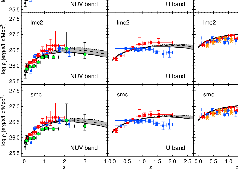
Figure 17.— NUV, U and V band comoving luminosity density calculated using best fit combination of SFRD($z$) and $A_{\rm FUV}(z)$ obtained using different extinction curves $k(\nu)$. For the references and plotting symbols see Table 1. Solid, dashed and dot-dashed lines represent values of the best fit $\rho_{\nu}$ calculated for the SFRD($z$) obtained using the low, median and high models, respectively. From top to bottom extinction curve used are Calzetti et al. (2000), Milky-Way, LMC, LMC2 and SMC, respectively.

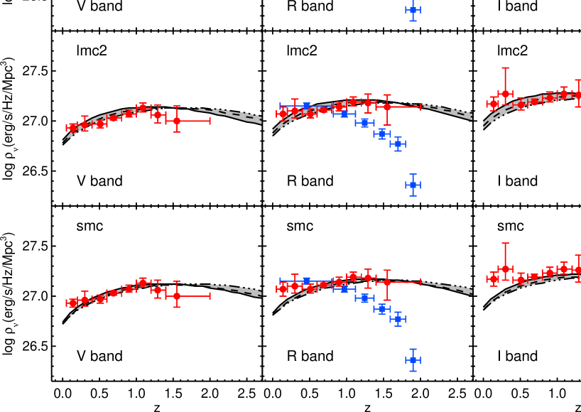
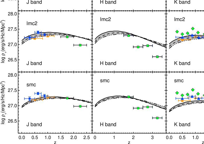
Figure 17.— … continued (for V, R and I band). For the references and plotting symbols see Table 1. Solid, dashed and dot-dashed lines represent values of the best fit $\rho_{\nu}$ calculated for the SFRD($z$) obtained using the low, median and high models, respectively. From top to bottom extinction curve used are Calzetti et al. (2000), Milky-Way, LMC, LMC2 and SMC, respectively.

Figure 17.— … continued (for J, H and K band). For the references and plotting symbols see Table 1. Solid, dashed and dot-dashed lines represent values of the best fit $\rho_{\nu}$ calculated for the SFRD($z$) obtained using the low, median and high models, respectively. From top to bottom extinction curve used are Calzetti et al. (2000), Milky-Way, LMC, LMC2 and SMC, respectively.

Table 5Observations of the Galaxy Luminosity Function

Reference	band	z	$\alpha$	Lmin	$\Delta_{1}$	$\Delta_{2}$	Reference	band	z	$\alpha$	Lmin	$\Delta_{1}$	$\Delta_{2}$
				(L∗)	%	%					(L∗)	%	%
Cucciati et al. (2012)	FUV	0.125	-1.05	0	1	3	Tresse et al. (2007)	U	0.14	-1.05	0	1	3
Tresse et al. (2007)	FUV	0.14	-1.13	0	1	4	Dahlen et al. (2005)	U	0.3	-1.31	0	4	9
Cucciati et al. (2012)	FUV	0.3	-1.17	0	2	5	Tresse et al. (2007)	U	0.3	-1.17	0	2	5
Schiminovich et al. (2005)	FUV	0.3	-1.19	0	2	6	Dahlen et al. (2005)	U	0.46	-1.2	0	2	6
Tresse et al. (2007)	FUV	0.3	-1.6	0	15	25	Tresse et al. (2007)	U	0.51	-1.17	0	2	5
Cucciati et al. (2012)	FUV	0.5	-1.07	0	1	3	Dahlen et al. (2005)	U	0.625	-1.31	0	4	9
Schiminovich et al. (2005)	FUV	0.5	-1.55	0	12	22	Tresse et al. (2007)	U	0.69	-1.27	0	3	8
Tresse et al. (2007)	FUV	0.51	-1.6	0	15	25	Dahlen et al. (2005)	U	0.875	-1.31	0	4	9
Tresse et al. (2007)	FUV	0.69	-1.6	0	15	25	Tresse et al. (2007)	U	0.9	-1.44	0	8	15
Cucciati et al. (2012)	FUV	0.7	-0.9	0	0	1	Dahlen et al. (2005)	U	0.97	-1.2	0	2	6
Schiminovich et al. (2005)	FUV	0.7	-1.6	0	15	25	Tresse et al. (2007)	U	1.09	-1.51	0	10	19
Cucciati et al. (2012)	FUV	0.9	-0.85	0	0	1	Dahlen et al. (2007)	U	1.245	-1.2	0	2	6
Tresse et al. (2007)	FUV	0.9	-1.6	0	15	25	Tresse et al. (2007)	U	1.29	-1.59	0	15	25
Schiminovich et al. (2005)	FUV	1	-1.6	0	15	25	Dahlen et al. (2005)	U	1.48	-1.2	0	2	6
Tresse et al. (2007)	FUV	1.09	-1.6	0	15	25	Tresse et al. (2007)	U	1.55	-1.68	0	21	32
Cucciati et al. (2012)	FUV	1.1	-0.91	0	0	2	Dahlen et al. (2005)	U	1.695	-1.2	0	2	6
Dahlen et al. (2007)	FUV	1.125	-1.48	0	9	17	Dahlen et al. (2005)	U	1.9	-1.2	0	2	6
Tresse et al. (2007)	FUV	1.29	-1.6	0	15	25	Tresse et al. (2007)	B	0.14	-1.09	0	1	4
Cucciati et al. (2012)	FUV	1.45	-1.09	0	1	4	Dahlen et al. (2005)	B	0.3	-1.37	0	5	11
Tresse et al. (2007)	FUV	1.55	-1.6	0	15	25	Tresse et al. (2007)	B	0.3	-1.15	0	2	5
Dahlen et al. (2007)	FUV	1.75	-1.48	0	9	17	Dahlen et al. (2005)	B	0.46	-1.28	0	3	8
Schiminovich et al. (2005)	FUV	2.0	-1.49	0	10	18	Tresse et al. (2007)	B	0.51	-1.22	0	2	6
Cucciati et al. (2012)	FUV	2.1	-1.3	0	4	9	Dahlen et al. (2005)	B	0.625	-1.37	0	5	11
Dahlen et al. (2007)	FUV	2.22	-1.48	0	9	17	Tresse et al. (2007)	B	0.69	-1.12	0	1	4
Reddy & Steidel (2009)a	FUV	2.3	-1.73	0.01	0	15	Dahlen et al. (2005)	B	0.875	-1.37	0	5	11
Schiminovich et al. (2005)	FUV	2.9	-1.47	0	9	16	Tresse et al. (2007)	B	0.9	-1.33	0	4	10
Cucciati et al. (2012)	FUV	3	-1.5	0	10	18	Dahlen et al. (2005)	B	0.97	-1.28	0	3	8
Reddy & Steidel (2009)a	FUV	3.05	-1.73	0.01	0	15	Tresse et al. (2007)	B	1.09	-1.40	0	6	13
Bouwens et al. (2011)b	FUV	3.8	-1.73	0.01	0	15	Dahlen et al. (2005)	B	1.245	-1.28	0	3	8
Cucciati et al. (2012)	FUV	4	-1.5	0	10	18	Tresse et al. (2007)	B	1.29	-1.48	0	9	17
Bouwens et al. (2011)b	FUV	5	-1.66	0.01	0	13	Dahlen et al. (2005)	B	1.48	-1.28	0	3	8
Bouwens et al. (2011)c	FUV	5.9	-1.74	0.01	0	16	Tresse et al. (2007)	B	1.55	-1.57	0	14	23
Bouwens et al. (2011)b	FUV	6.8	-2.01	0.01	0	27	Dahlen et al. (2005)	B	1.695	-1.28	0	3	8
Bouwens et al. (2011)d	FUV	8	-1.91	0.01	0	22	Dahlen et al. (2005)	B	1.9	-1.28	0	3	8
Wyder et al. (2005)	NUV	0.055	-1.16	0	2	5	Faber et al. (2007)	B	0.3	-1.3	0.01	0	5
Cucciati et al. (2012)	NUV	0.125	-1.08	0	1	4	Faber et al. (2007)	B	0.5	-1.3	0.01	0	5
Tresse et al. (2007)	NUV	0.14	-1.32	0	4	9	Faber et al. (2007)	B	0.7	-1.3	0.01	0	5
Cucciati et al. (2012)	NUV	0.3	-1.02	0	1	3	Faber et al. (2007)	B	0.9	-1.3	0.01	0	5
Tresse et al. (2007)	NUV	0.3	-1.32	0	4	9	Faber et al. (2007)	B	1.1	-1.3	0.01	0	5
Dahlen et al. (2007)	NUV	0.33	-1.39	0	6	12	Tresse et al. (2007)	V	0.14	-1.15	0	2	5
Cucciati et al. (2012)	NUV	0.5	-1.08	0	1	4	Tresse et al. (2007)	V	0.3	-1.21	0	2	6
Tresse et al. (2007)	NUV	0.51	-1.32	0	4	9	Tresse et al. (2007)	V	0.51	-1.35	0	5	11
Dahlen et al. (2007)	NUV	0.545	-1.39	0	6	12	Tresse et al. (2007)	V	0.69	-1.35	0	5	11
Tresse et al. (2007)	NUV	0.69	-1.32	0	4	9	Tresse et al. (2007)	V	0.9	-1.50	0	10	18
Cucciati et al. (2012)	NUV	0.7	-0.95	0	0	2	Tresse et al. (2007)	V	1.09	-1.57	0	14	23
Cucciati et al. (2012)	NUV	0.9	-0.81	0	0	1	Tresse et al. (2007)	V	1.29	-1.65	0	19	30
Tresse et al. (2007)	NUV	0.9	-1.32	0	4	9	Tresse et al. (2007)	V	1.55	-1.74	0	27	38
Tresse et al. (2007)	NUV	1.09	-1.32	0	4	9	Tresse et al. (2007)	R	0.14	-1.16	0	2	5
Cucciati et al. (2012)	NUV	1.1	-0.88	0	0	1	Tresse et al. (2007)	R	0.3	-1.27	0	3	8
Dahlen et al. (2007)	NUV	1.125	-1.39	0	6	12	Dahlen et al. (2005)	R	0.46	-1.30	0	4	9
Tresse et al. (2007)	NUV	1.29	-1.32	0	4	9	Tresse et al. (2007)	R	0.51	-1.42	0	7	14
Cucciati et al. (2012)	NUV	1.45	-1.05	0	1	3	Tresse et al. (2007)	R	0.69	-1.41	0	7	13
Tresse et al. (2007)	NUV	1.55	-1.32	0	4	9	Tresse et al. (2007)	R	0.9	-1.53	0	11	20
Dahlen et al. (2007)	NUV	1.75	-1.39	0	6	12	Dahlen et al. (2005)	R	0.97	-1.30	0	4	9
Cucciati et al. (2012)	NUV	2.1	-1.16	0	2	5	Tresse et al. (2007)	R	1.09	-1.60	0	15	25
Dahlen et al. (2007)	NUV	2.225	-1.39	0	6	12	Dahlen et al. (2005)	R	1.245	-1.30	0	4	9
Cucciati et al. (2012)	NUV	3	-1.15	0	2	5	Tresse et al. (2007)	R	1.29	-1.68	0	21	32

Wavelengths at different bands are: FUV=0.15$\mu$m, NUV=0.28$\mu$m, U=0.365$\mu$m, B=0.445$\mu$m, V=0.551$\mu$m, R=0.658$\mu$m
$\Delta_{1}=(a_{0}-a_{1})/a_{0}$ and $\Delta_{2}=(a_{0}-a_{2})/a_{0}$ where $a_{0}=\Gamma(\alpha+2,L_{min}/L^{*})$, $a_{1}=\Gamma(\alpha+2,0.01)$, and $a_{2}=\Gamma(\alpha+2,0.03)$
^a The corresponding wavelength is 1700Å.
^b The corresponding wavelength is 1600Å. ^c The corresponding wavelength is 1350Å. ^d The corresponding wavelength is 1750Å.

Table 5…(continue) Observations of the Galaxy Luminosity Function

Reference	band	z	$\alpha$	Lmin	$\Delta_{1}$	$\Delta_{2}$	Reference	band	z	$\alpha$	Lmin	$\Delta_{1}$	$\Delta_{2}$
				(L∗)	%	%					(L∗)	%	%
Dahlen et al. (2005)	R	1.48	-1.30	0	4	9	SM13	H	1.75	-1.30	0.01	0	5
Tresse et al. (2007)	R	1.55	-1.77	0	29	42	SM13	H	2.25	-1.23	0.01	0	4
Dahlen et al. (2005)	R	1.695	-1.30	0	4	9	SM13	H	2.75	-1.11	0.01	0	2
Dahlen et al. (2005)	R	1.9	-1.30	0	4	9	SM13	H	3.35	-1.30	0.01	0	5
Tresse et al. (2007)	I	0.14	-1.19	0	2	6	Smith et al. (2009)	K	0.155	-0.81	0.01	0	1
Tresse et al. (2007)	I	0.3	-1.32	0	4	9	Arnouts et al. (2007)	K	0.30	-1.1	0.01	0	2
Tresse et al. (2007)	I	0.51	-1.47	0	9	16	Arnouts et al. (2007)	K	0.50	-1.1	0.01	0	2
Tresse et al. (2007)	I	0.69	-1.41	0	7	13	Cirasuolo et al. (2007)	K	0.5	-0.99	0.01	0	1
Tresse et al. (2007)	I	0.9	-1.52	0	11	19	Pozzetti et al. (2003)	K	0.5	-1.25	0.02	-2	2
Tresse et al. (2007)	I	1.09	-1.59	0	15	25	Arnouts et al. (2007)	K	0.70	-1.1	0.01	0	2
Tresse et al. (2007)	I	1.29	-1.67	0	20	31	Cirasuolo et al. (2007)	K	0.875	-1.00	0.01	0	1
Tresse et al. (2007)	I	1.55	-1.76	0	28	41	Arnouts et al. (2007)	K	0.90	-1.1	0.01	0	2
Dahlen et al. (2005)	J	0.3	-1.48	0	9	17	Pozzetti et al. (2003)	K	1	-0.98	0.02	0	0
Pozzetti et al. (2003)	J	0.5	-1.22	0.02	-2	1	Cirasuolo et al. (2007)	K	0.875	-1.00	0.01	0	1
Dahlen et al. (2005)	J	0.625	-1.48	0	9	17	Arnouts et al. (2007)	K	1.10	-1.1	0.01	0	2
Dahlen et al. (2005)	J	0.875	-1.48	0	9	17	Cirasuolo et al. (2007)	K	1.125	-0.94	0.01	0	1
Pozzetti et al. (2003)	J	1	-0.86	0.02	0	0	Arnouts et al. (2007)	K	1.35	-1.1	0.01	0	2
SM13 d	J	1.75	-1.24	0.01	0	4	Cirasuolo et al. (2007)	K	1.375	-0.92	0.01	0	1
SM13	J	2.25	-1.12	0.01	0	2	Cirasuolo et al. (2007)	K	1.625	-1	0.01	0	1
SM13	J	2.75	-1.17	0.01	0	3	Arnouts et al. (2007)	K	1.75	-1.1	0.01	0	2
SM13	J	3.35	-0.92	0.01	0	1	Cirasuolo et al. (2007)	K	2	-1	0.01	0	1

Wavelengths at different wavebands are: R=0.658$\mu$m, I=0.806$\mu$m, J=1.27$\mu$m, H=1.63$\mu$m and K=2.2$\mu$m.
$\Delta_{1}=(a_{0}-a_{1})/a_{0}$ and $\Delta_{2}=(a_{0}-a_{2})/a_{0}$ where $a_{0}=\Gamma(\alpha+2,L_{min}/L^{*})$, $a_{1}=\Gamma(\alpha+2,0.01)$, and $a_{2}=\Gamma(\alpha+2,0.03)$
^d The acronym SM13 corresponds to the reference Stefanon & Marchesini (2013)

References

- Ackermann et al. (2012) Ackermann, M., Ajello, M., Allafort, A., et al. 2012, Science, 338, 1190
- Amblard et al. (2010) Amblard, A., Cooray, A., Serra, P., et al. 2010, A&A, 518, L9
- Arlen et al. (2012) Arlen, T. C., Vassiliev, V. V., Weisgarber, T., Wakely, S. P., & Yusef Shafi, S. 2012, ArXiv e-prints, arXiv:1210.2802
- Arnouts et al. (2007) Arnouts, S., Walcher, C. J., Le Fèvre, O., et al. 2007, A&A, 476, 137
- Baldry & Glazebrook (2003) Baldry, I. K., & Glazebrook, K. 2003, ApJ, 593, 258
- Behroozi et al. (2013) Behroozi, P. S., Wechsler, R. H., & Conroy, C. 2013, ApJ, 770, 57
- Bernstein et al. (2002) Bernstein, R. A., Freedman, W. L., & Madore, B. F. 2002, ApJ, 571, 56
- Berta et al. (2010) Berta, S., Magnelli, B., Lutz, D., et al. 2010, A&A, 518, L30
- Béthermin et al. (2010) Béthermin, M., Dole, H., Beelen, A., & Aussel, H. 2010, A&A, 512, A78
- Bouwens et al. (2007) Bouwens, R. J., Illingworth, G. D., Franx, M., & Ford, H. 2007, ApJ, 670, 928
- Bouwens et al. (2009) Bouwens, R. J., Illingworth, G. D., Franx, M., et al. 2009, ApJ, 705, 936
- Bouwens et al. (2011) Bouwens, R. J., Illingworth, G. D., Labbe, I., et al. 2011, Natur, 469, 504
- Bouwens et al. (2012) Bouwens, R. J., Illingworth, G. D., Oesch, P. A., et al. 2012, ApJ, 754, 83
- Buat et al. (2012) Buat, V., Noll, S., Burgarella, D., et al. 2012, A&A, 545, A141
- Burgarella et al. (2013) Burgarella, D., Buat, V., Gruppioni, C., et al. 2013, A&A, 554, A70
- Calzetti (2001) Calzetti, D. 2001, PASP, 113, 1449
- Calzetti et al. (2000) Calzetti, D., Armus, L., Bohlin, R. C., et al. 2000, ApJ, 533, 682
- Calzetti et al. (1994) Calzetti, D., Kinney, A. L., & Storchi-Bergmann, T. 1994, ApJ, 429, 582
- Chabrier (2003) Chabrier, G. 2003, PASP, 115, 763
- Chevallard et al. (2013) Chevallard, J., Charlot, S., Wandelt, B., & Wild, V. 2013, MNRAS, 432, 2061
- Cirasuolo et al. (2007) Cirasuolo, M., McLure, R. J., Dunlop, J. S., et al. 2007, MNRAS, 380, 585
- Clayton & Martin (1985) Clayton, G. C., & Martin, P. G. 1985, ApJ, 288, 558
- Cole et al. (2001) Cole, S., Norberg, P., Baugh, C. M., et al. 2001, MNRAS, 326, 255
- Condon et al. (2002) Condon, J. J., Cotton, W. D., & Broderick, J. J. 2002, AJ, 124, 675
- Cooray et al. (2004) Cooray, A., Bock, J. J., Keatin, B., Lange, A. E., & Matsumoto, T. 2004, ApJ, 606, 611
- Cucciati et al. (2012) Cucciati, O., Tresse, L., Ilbert, O., et al. 2012, A&A, 539, A31
- Dahlen et al. (2007) Dahlen, T., Mobasher, B., Dickinson, M., et al. 2007, ApJ, 654, 172
- Dahlen et al. (2005) Dahlen, T., Mobasher, B., Somerville, R. S., et al. 2005, ApJ, 631, 126
- Dale et al. (2007) Dale, D. A., Gil de Paz, A., Gordon, K. D., et al. 2007, ApJ, 655, 863
- Dale et al. (2012) Dale, D. A., Aniano, G., Engelbracht, C. W., et al. 2012, ApJ, 745, 95
- de Jager et al. (1994) de Jager, O. C., Stecker, F. W., & Salamon, M. H. 1994, Natur, 369, 294
- Dole et al. (2006) Dole, H., Lagache, G., Puget, J.-L., et al. 2006, A&A, 451, 417
- Domínguez et al. (2013) Domínguez, A., Finke, J. D., Prada, F., et al. 2013, ApJ, 770, 77
- Domínguez & Prada (2013) Domínguez, A., & Prada, F. 2013, ApJ, 771, L34
- Domínguez et al. (2011) Domínguez, A., Primack, J. R., Rosario, D. J., et al. 2011, MNRAS, 410, 2556
- Dwek & Arendt (1998) Dwek, E., & Arendt, R. G. 1998, ApJ, 508, L9
- Dwek & Krennrich (2013) Dwek, E., & Krennrich, F. 2013, Astroparticle Physics, 43, 112
- Dwek & Slavin (1994) Dwek, E., & Slavin, J. 1994, ApJ, 436, 696
- Faber et al. (2007) Faber, S. M., Willmer, C. N. A., Wolf, C., et al. 2007, ApJ, 665, 265
- Fazio et al. (2004) Fazio, G. G., Ashby, M. L. N., Barmby, P., et al. 2004, ApJS, 154, 39
- Finkbeiner et al. (2000) Finkbeiner, D. P., Davis, M., & Schlegel, D. J. 2000, ApJ, 544, 81
- Finke et al. (2010) Finke, J. D., Razzaque, S., & Dermer, C. D. 2010, ApJ, 712, 238
- Fixsen et al. (1998) Fixsen, D. J., Dwek, E., Mather, J. C., Bennett, C. L., & Shafer, R. A. 1998, ApJ, 508, 123
- Franceschini et al. (2008) Franceschini, A., Rodighiero, G., & Vaccari, M. 2008, A&A, 487, 837
- Frank & Péroux (2010) Frank, S., & Péroux, C. 2010, MNRAS, 406, 2235
- Gilmore et al. (2009) Gilmore, R. C., Madau, P., Primack, J. R., Somerville, R. S., & Haardt, F. 2009, MNRAS, 399, 1694
- Gilmore et al. (2012) Gilmore, R. C., Somerville, R. S., Primack, J. R., & Domínguez, A. 2012, MNRAS, 422, 3189
- Gordon et al. (2003) Gordon, K. D., Clayton, G. C., Misselt, K. A., Landolt, A. U., & Wolff, M. J. 2003, ApJ, 594, 279
- Gould & Schréder (1966) Gould, R. J., & Schréder, G. 1966, Physical Review Letters, 16, 252
- Gruppioni et al. (2013) Gruppioni, C., Pozzi, F., Rodighiero, G., et al. 2013, MNRAS, 432, 23
- Haardt & Madau (1996) Haardt, F., & Madau, P. 1996, ApJ, 461, 20
- Haardt & Madau (2012) —. 2012, ApJ, 746, 125
- Hauser & Dwek (2001) Hauser, M. G., & Dwek, E. 2001, AR&A, 39, 249