A simple spin model for three steps relaxation and secondary proccesses in glass formers

Abstract

A number of general trends are known to occur in systems displaying secondary processes in glasses and glass formers. Universal features can be identified as components of large and small cooperativeness whose competition leads to excess wings or apart peaks in the susceptibility spectrum. To the aim of understanding such rich and complex phenomenology we analyze the behavior of a model combining two apart glassy components with a tunable different cooperativeness. The model salient feature is, indeed, based on the competition of the energetic contribution of groups of dynamically relevant variables, e.g., density fluctuations, interacting in small and large sets. We investigate how the model is able to reproduce the secondary processes physics without further ad hoc ingredients, displaying known trends and properties under cooling or pressing.

1 Introduction

In several supercooled liquids and glasses processes are observed whose typical timescales are much longer than cage rattling microscopic motion and local rearrangement timescales of the so-called (fast) $\beta$ processes and, yet are much shorter than the time-scale of structural relaxation, i.e., of the $\alpha$ processes. These are usually termed “Secondary processes” and are related to complicated though local (non-cooperative or not fully cooperative) dynamics. We will, in particular, investigate Johari-Goldstein processes [1], for which special properties hold, such as dependence of their relaxation time on density and temperature and a strict relationship to structural processes [2]. In the present paper we will term them simply as $\beta$, referring to fast $\beta$ processes as $\gamma$. Their existence was first pointed out in the 1960’s from dielectric loss spectra measurements, in which they are identified by the occurrence of a second peak at a frequency higher than the frequency $\nu_{\alpha}$ of the $\alpha$ processes peak. This so-called $\beta$-peak has been recorded in a large number of substances as, e.g., poly-alcohols [3, 4, 5] mixtures of rigid polar molecules and oligomers [6, 7, 8, 9], propylene glycols [10] and many others comprehensively gathered in Ref. [11].

Also in cases where the spectral density of response losses do not clearly show a second peak, secondary processes are nkown to be active and their presence is, then, identified, by some anomaly at frequency higher than $\nu_{\alpha}$, called excess wing [12, 13]. Though it was initially observed as an apart phenomenon [14], more recent investigation has shown that the excess wings rather are manifestations of $\beta$ JG processes [15, 8, 11]. Properly tuning external parameters (temperature, pressure, concentration, …) $\beta$-peaks can come out of the excess wings or, viceversa, secondary peaks can reduce to excess wings. According to Cummins [16] the relevant parameter to tune in passing from one scenario to the other one might be the rotation-translation coupling constant, becoming stronger as density increases, and being larger for a liquid glass former made of elongated and strongly anisotropic molecules.

Theoretical attempts have been carried out in this direction in the framework of Mode Coupling Theory (MCT). According to this theory the relaxation of reorientational correlation and rotation-translation coupling in liquids composed of strongly anisotropic molecules appears to be logarithmic in time [17]. A comprehensive picture is, though, not yet established and many questions are open. For instance, about the dependence of the characteristic time-scales of JG processes on temperature and pressure, else, on concentration. Or about the chance that secondary processes might disclose a certain degree of cooperativeness [18], or the explanation for the persistence of the $\beta$ processes also below the calorimetric glass transition temperature $T_{g}$. A very interesting question is whether there is a straightforward connection, and, in case, which one, between processes evolving at qualitatively different time-scales. Were it the case, one might devise the long-time behavior of $\alpha$ relaxation from the behaviors of the fast small-amplitude cage dynamics ($\gamma$ processes) and of the $\beta$ secondary processes. In glasses, and glass formers, where $\alpha$ and $\beta$ peaks of the loss spectra can be clearly resolved in frequency one can resort to a description based on two time-scale bifurcation accelerations as temperature is lowered. Processes consequently evolve on three well-separated time sectors. Examples of well resolved peak separation can be found, e.g., in are 4-polybutadiene, toluene [19] , sorbitol [5] mixture of quinaldine in tri-styrene [6, 8, 7] or trimer propilene glycol [10].

A way to reproduce secondary processes, or at least some stretching in the high frequency side of the $\alpha$ relaxation, is to include the coupling of correlators of two different components, such has the density correlators of tagged particles and their surrounding medium [20]. In the limit of strong coupling between correlators it is possible to to yield a Cole-Cole law for the loss spectrum in the limit [21], but no distinct apart secondary $\beta$ peak is resolved. To the aim of overcoming these limitations in the theoretical description of secondary processes we propose a model with a single component but a dynamic kernel corresponding to two different kinds of cooperativeness.

2 The model

The model we shall discuss is known as the Spherical $s+p$ Spin Glass model defined by the Hamiltonian

$${\cal H}= -\!\sum_{i_{1}<\ldots<i_{s}}\!J^{(s)}_{i_{1}\ldots i_{s}}\sigma_{i_{1}}\cdots\sigma_{i_{s}}$$

$$-\!\sum_{i_{1}<\ldots<i_{p}}\!J^{(p)}_{i_{1}\ldots i_{p}}\sigma_{i_{1}}\cdots\sigma_{i_{p}}$$

where $J^{(t)}_{i_{1}\ldots i_{t}}$ ($t=s,p$ with $s<p$ for convention) are uncorrelated, zero mean, Gaussian variables of variance

$${\overline{\left(J^{(t)}_{i_{1}\ldots i_{t}}\right)^{2}}}=\frac{J_{t}^{2}t!}{2N^{t-1}}$$ (2)

where the overbar denotes the average over the quenched disorder and $\sigma_{i}$ are $N$ continuous real variables (spins) ranging from $-\infty$ to $+\infty$ obeying the global constraint $\sum_{i}\sigma_{i}^{2}=N$ (spherical constraint). The model, defined on a complete graph, is intrinsically mean-field. Indeed, each spin interacts with all others and no geometric nor dimensional structure is relevant for the interaction network. In order to guarantee thermodynamic convergence and an extensive energy the interaction magnitude is very small, and scales with the system size as $J_{i_{1},\ldots,i_{t}}\sim 1/{N}^{(t-1)/2}$.

2.1 A bit of thermodynamics

Due to the mean-field nature of the model the metastable glassy states responsible for the dynamic arrest can be studied by means of thermodynamics. Indeed, in these spherical spin models with quenched disordered couplings, the configurational entropy, related to the number of metastable states, is a true, static, thermodynamic state function, unlike realistic structural glasses [22]. Therefore, to make connection with glass formers, we first recall some results on the model static properties, both in its ideal glassy phase and in the supercooled liquid phase. Let us define the overlap

$$q_{\alpha\beta}\equiv\frac{1}{N}\sum_{i=1}^{N}\langle\sigma_{i}\rangle_{\alpha}\langle\sigma_{i}\rangle_{\beta}$$ (3)

between any two glassy stable or metastable states $\alpha$ and $\beta$ whose equilibrium measure in the corresponding ergodic component is labeled by $\langle\ldots\rangle_{\alpha,\beta}$.

In a cooling procedure, these states first occur as excited metastable states at the temperature $T=T_{\rm d}=T_{\rm mct}$ coinciding with the dynamic or mode coupling temperature. Physically, this is the temperature at which the glassy states dominate the free energy landscape through which the system dynamics takes place. At this temperature their number becomes macroscopic, i.e., exponentially large woth the system size, and the configurational entropy (also called complexity) becomes extensive with the system size $N$.

Below $T=T_{\rm d}=T_{\rm mct}$ the phase space breaks down into several regions (glass phase), and the overlap $q_{\alpha\beta}$ takes different values $q_{\kappa}$, with probability $p_{\kappa}$. The number of different values depends on both the region of the phase diagram and the values of $s$ and $p$, and can be finite or infinite. In the first case the phase is called $R$ Replica Symmetry Broken ($R$RSB), where $R$ is the number of different values of $q_{\alpha\beta}$, while in the second case it is termed Full Replica Symmetry Broken (FRSB). Mixed phases are also possible [23, 24].

Here, we focus on the cases where secondary processes show up. As it will be later clarified, these correspond to a static description in which $q_{\alpha\beta}$ takes two non-trivial value ($R=2$) with probability:

$$\begin{split}P(q)=p_{1}\delta(q)&+(p_{2}-p_{1})\,\delta(q-q_{1})\\ &+(1-p_{2})\,\delta(q-q_{2}).\end{split}$$ (4)

In terms of free energy lanscape, this picture displays a hierarchical structure where each glassy minimum - representing a separated ergodic component - also contains a further set of glassy minima inside, as pictorially represented in Fig. 1, cf. Ref. [25]. Inner states have higher overlap $q_{2}$ while outer states have lower overlap, $q_{1}<q_{2}$. Such “nested” minima appear as metastable states at the tricritical point along the dynamic (swallowtail) arrest line. They become the ideal equilibrium stable glass states at the static - Kauzmann - transition line. As the dynamic arrest line is approached, e.g., by cooling, far from the tricritical point only one set of states appear. This implies that only one kind of diverging timescale occurs for slow processes, the structural ones.

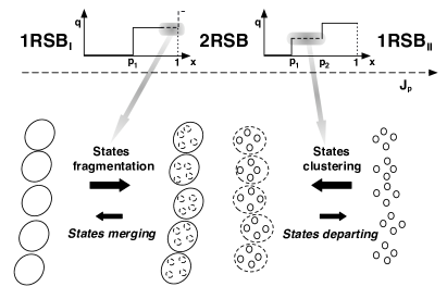
Figure 1: Pictorial representation of the inverse $q(x)$ of the cumulative function $x(q)$ of the $P(q)$ defined in Eq. (4) as $J_{p}$ is increased keeping $J_{s}$ fixed. Below, the inner and outer states in the 2RSB case are shown along with their “generation” by fragmentation or clustering moving from 1RSB sectors of the phase diagram, where no secondary processes occur.

The values of $q_{1}$ and $q_{2}$ are given by the solution of the self-consistent equations [26, 25]:

$${\cal M}(q_{1})=\frac{q_{2}-q_{1}}{\chi(q_{1})\,\chi(0)},$$ (5)

$${\cal M}(q_{2})-{\cal M}(q_{1})=\frac{q_{2}-q_{1}}{\chi(q_{2})\,\chi(q_{1})},$$ (6)

where

$$\chi(q_{2}) = 1-q_{2},$$

$$\chi(q_{1}) = \chi(q_{2})+p_{2}(q_{2}-q_{1}),$$

$$\chi(0) = \chi(q_{1})+p_{1}q_{1},$$

and where we have introduced the functions

$$g(X)=\frac{v_{s-1}}{s}X^{s}+\frac{v_{p-1}}{p}X^{p},$$ (7)

$${\cal M}(X)=g^{\prime}(X)=v_{s-1}X^{s-1}+v_{p-1}X^{p-1}$$ (8)

with

$$v_{t-1} = t\beta^{2}J_{t}^{2}/2.$$ (9)

In a pure static study, the thermodynamics is ruled by the states that extremize the free energy, and this leads to the two additional self-consistent equations (static condition)

$$g(q_{2})-g(q_{1})=(q_{2}-q_{1})\left[{\cal M}(q_{1})-\frac{1}{p_{2}\chi(q_{1})}\right]$$

$$\hskip 28.45274pt-\frac{1}{p_{2}^{2}}\ln\frac{\chi(q_{2})}{\chi(q_{1})},$$ (10)

$$g(q_{1})=-\frac{q_{1}}{p_{1}\chi(0)}-\frac{1}{p_{1}^{2}}\ln\frac{\chi(q_{1})}{\chi(0)},$$ (11)

which fix the value of $p_{1}$ and $p_{2}$. Non-trivial solutions of these equations appear at the static (else called Kauzmann) critical temperature $T=T_{K}<T_{\rm d}$.

To account for the metastable states that dominate the dynamics in the $2$RSB phase for temperatures $T\in[T_{K},T_{\rm d}]$, equations (10,11) must be replaced by

$${\cal M}^{\prime}(q_{\kappa})=\frac{1}{(1-q_{\kappa})^{2}},\quad\kappa=1,2$$ (12)

which follows from the requirement that the solution maximizes the complexity [27]. This condition ensures that the dynamics ruled by the memory kernel ${\cal M}(\phi)$ be marginally stable [26]. It is known as the marginal condition because it coincides with the marginal stability condition in the solution of the statics of the model [28]. It bridges the static and dynamic properties in the $2$RSB phase, where $q_{1}$ and $q_{2}$ become the two nontrivial asymptotic plateau values, i. e., non-ergodicity factors, of the dynamic correlation function in the three steps relaxation scenario.

Away from the $2$RSB phase, only one plateau occurs. In these cases the solutions to the above equations coincide $q_{1}=q_{2}$. Beyond the dynamic critical line glass-to-glass transitions can occur, between $1$RSB and $2$RSB kind of glasses. Here we are mainly interested in the equilibrium dynamics of supercolled liquids. The interested reader in the frozen glass phase can look, e.g., at Refs. [24, 26].

2.2 Dynamic phase diagrams and swallowtail singularity

The existence of two nontrivial asymptotic plateau’s of the dynamic correlation function, approaching the $2$RSB phase, is associated with the presence of a given type of singularity in the dynamic equations. According to Arnold’s classification of singular points in catastrophe theory, the model has to display a double bifurcation $A_{4}$, or swallowtail, singularity.

A static glass $2$RSB phase in the spherical $s+p$ spin glass model can, actually, be found provided $s$ and $p$ are equal or larger than the solution of

$$(p^{2}+s^{2}+p+s-3ps)^{2}-ps(p-2)(s-2)=0,$$ (13)

as it has been shown in Ref. [26]. Some threshold values of $(s,p)$ are $(3,8)$, $(4,11)$ or $(5,16)$. The larger $p-s$, the broader the region of phase diagram where the static $2$RSB phase can be found. This is a necessary condition for the occurrence of a $2$RSB phase somewhere in the static (thermodynamic) phase diagram but do not guarantee the occurrence of an $A_{4}$ singularity along the dynamic arrest line.

To have a $2$RSB phase accessible in the MCT equilibrium dynamics - i.e., a swallowtail singularity along the dynamic arrest line - the condition on $s$ and $p$ is stronger [29]:

$$\sqrt{(s-1)(p-1)}-\sqrt{(p-2)(s-2)}\geq\sqrt{2}.$$ (14)

In this case a the $A_{4}$ point is exposed to the fluid phase and a three step correlation function, or three peak loss function, develops approaching the dynamic transition next to this point. Some lower bound values are $(s,p)=(3,10)$, $(4,16)$, $(5,22)$.

Moreover, in order to have a swallowtail also in the static-Kauzmann transition line the parameters $s$ and $p$ must further satisfy the equation

$$(sp-p-s+1)y^{2}-(p+s+1)y+2\geq 0$$ (15)

where $y\in[0,1]$ is solution of

$$(sp-p-s-1)y+p+s-1=sp\,z(y)$$ (16)

and $z(y)$ is the CS $z$-function [30]

$$z(y)=-2y\frac{1-y+\ln y}{(1-y)^{2}}.$$ (17)

Some critical values $(s,p)$: $(3,13)$, $(4,23)$, $(5,35)$. In this case the stable ideal 2RSB phase can be accessed directly from the stable fluid phase.

Relevant external parameters for the phase diagram will be the “concentration” of large cooperativeness $\rho$, defined as

$$J_{p} = \rho J\quad;\quad J_{s}=(1-\rho)J$$ (18)

$$J = J_{s}+J_{p}$$ (19)

and the temperature, defined in units of the small cooperativeness interaction $J_{s}$,

$$\frac{T}{J_{s}}=\sqrt{\frac{s}{2v_{s-1}}}$$ (20)

Transition lines can be drawn parametrically in the overlap variable $q\in[0,1]$ at the dynamic arrest fold singularity, cf. Fig. 2: [31]

$$v_{p-1} = \frac{(s-1)q-(s-2)}{(p-s)q^{p}-2(1-q)^{2}}$$ (21)

$$v_{s-1} = \frac{(p-1)q-(p-2)}{(p-s)q^{s}-2(1-q)^{2}}$$ (22)

or in $T,\rho$ using the transformations Eqs. (9), (20), as shown in Fig. 3.

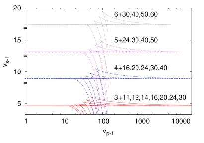
Figure 2: Dynamic phase diagrams in the $v_{s},v_{p}$ plane. The dynamic lines with swallow tail are represented for series of models with $s=3,4,5$ and $6$.

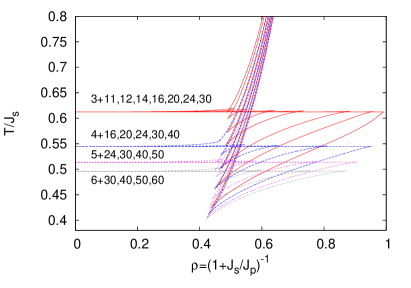
Figure 3: Dynamic phase diagrams in the $T/J_{s},\rho$ plane for different sets of models.

3 Dynamics equations

To study the slowing down of the dynamics as the critical arrest is approached from the liquid phase, we cannot rely only on the static analysis and the dynamics of the model must be analyzed. The relaxation dynamics of the system is described by the Langevin equation

$$\Gamma_{0}^{-1}\frac{\partial\sigma_{k}(t)}{\partial t}=-\frac{\delta{\cal H}[\{\sigma\}]}{\delta\sigma_{k}(t)}+\eta_{k}(t)$$ (23)

$$\qquad\langle\eta_{k}(t)\eta_{n}(t^{\prime})\rangle=2k_{B}T\Gamma_{0}^{-1}\delta_{kn}\delta(t-t^{\prime})$$

where $\eta_{k}$ is the thermal white noise and $\Gamma_{0}^{-1}$ is the microscopic time-scale. Using the Martin-Siggia-Rose response field approach in the path-integral formalism [32, 33], the average over the quenched disorder can be performed, and the equations of motion reduce to the self-consistent dynamics of single variable $\sigma(t)$. The fundamental observables to study the onset of the dynamic slowing down are the diagonal spin-spin time correlation function $C(t,t^{\prime})$ and the spin-response function $G(t,t^{\prime})$, which for our model are defined as

$$C(t,t^{\prime}) = {\overline{\langle\sigma(t)\sigma(t^{\prime})\rangle}},$$ (24)

$$G(t,t^{\prime}) = \left.\frac{\delta\overline{\langle\sigma(t)\rangle}}{\delta\beta h(t^{\prime})}\right|_{h=0},\qquad t>t^{\prime},$$ (25)

with $C(t,t)=1$ from the spherical constraint. The brackets denote the thermal average over different trajectories (and initial conditions). For temperature above $T_{\rm d}$ the dynamics is time translational invariant (TTI) and the response and correlation functions are related by the Fluctuation - Dissipation Theorem (FDT):

$$G(t-t^{\prime})=\theta(t-t^{\prime})\frac{\partial C(t-t^{\prime})}{\partial t^{\prime}}.$$ (26)

In this case, and using the shorthands $F^{\prime}(t)\equiv\partial F(t)/\partial t$, the dynamic equation for $C(t-t^{\prime})$ takes the form

$$\Gamma_{0}^{-1}\partial_{t}C(t)+\bar{r}C(t)+\int_{0}^{t}dt^{\prime}{\cal M}[C(t-t^{\prime})]\,C^{\prime}(t^{\prime})$$

$$\hskip 113.81102pt=\bar{r}-1$$ (27)

with initial the condition $C(t=0)=1$ and

$$\bar{r}=r-{\cal M}[C(t=0)]$$ (28)

The parameter $r$ in the above equation is a “bare mass” [34] related to the Lagrange multiplier needed to impose the spherical constraint [35]. The value of $\bar{r}$ can depend on temperature and on $\rho$ through ${\cal M}[C(t=0)]$. However, above $T_{d}$, $\bar{r}$ is constant and equal to $1$, so that the r.h.s. of (27) vanishes.

The kernel memory function ${\cal M}(t)\equiv{\cal M}[C(t)]$ for the spherical $s+p$ spin glass model we are considering has the functional form shown in Eq. (8). We stress that eq. (27) (with $\bar{r}=1$) is the equation governing the time correlation function in a schematic mode-coupling theory in which the second order time derivative term of the Mode Couplings equations is replaced by a first order one [36, 37].

To discuss the slowing down of the dynamics as the critical point is approached it is, further, useful to introduce the function $\bar{r}(q)$ [30]

$$\bar{r}(q)\equiv\frac{1}{1-q}-{\cal M}(q),$$ (29)

which determines the asymptotic value of the correlation function. Indeed, it can be shown that in the long time limit the asymptotic value $q=\lim_{t\to\infty}C(t)$ of the correlator $C(t)$ solution of Eq. (27) is given by the condition:

$$\bar{r}(q)=\bar{r}.$$ (30)

where $\bar{r}$ is the parameter appearing in Eq. (27) and defined in Eq. (28). The additional requirement for a critical dynamics, the marginal condition, imposes that $\bar{r}(q)$ be a local minimum with $\bar{r}^{\prime}(q)=0$ for $q$ solution of Eq. (30). When this happens $C(t)$ develops a plateau at $C(t)=q$, or multiple plateaus if more solutions to Eq. (30) become marginal simultaneously, as it is the case of the $2$RSB phase that we are discussing.

The properties of the dynamics close to the critical point can be analyzed by writing $C(t)=q+\phi(t)$, where $q$ is generic for the moment, and expanding ${\cal M}[C(t)]$ for small $\phi$:

$${\cal M}(q+\phi)=\sum_{m=0}^{\infty}\frac{{\cal M}^{(m)}(q)}{m!}\phi^{m}$$ (31)

where

$$\begin{split}{\cal M}^{(m)}&=\frac{d^{m}{\cal M}(q)}{dq^{m}}\\ &=\frac{m!}{(1-q)^{m+1}}-\frac{d^{m}\bar{r}(q)}{dq^{m}}.\end{split}$$ (32)

The integral term in Eq. (27) then reads

$$\int_{0}^{t}dt^{\prime}{\cal M}[C(t-t^{\prime})]C^{\prime}(t^{\prime})=$$

$$\sum_{m=1}^{\infty}\left[\frac{{\cal M}^{m-1}(q)}{(m-1)!}-(1-q)\frac{{\cal M}^{m}(q)}{m!}\right]\phi^{m}(t)$$

$$-(1-q){\cal M}(q)+\sum_{m=1}^{\infty}\frac{{\cal M}^{m}(q)}{m!}I_{m}(t)$$ (33)

where

$$I_{m}(t)\equiv\int_{0}^{t}\,dt^{\prime}\,\left[\phi^{m}(t-t^{\prime})-\phi^{m}(t)\right]\phi^{\prime}(t^{\prime}),$$ (34)

leading, after few algebraic manipulations, to:

$$\Gamma_{0}^{-1}\phi^{\prime}(t)+\left[\bar{r}+{\cal M}(q)-(1-q){\cal M}^{(1)}(q)\right]\phi(t)$$

$$\quad+\sum_{m=2}^{\infty}\left[\frac{{\cal M}^{(m-1)}}{(m-1)!}-(1-q)\frac{{\cal M}^{(m)}(q)}{m!}\right]\phi^{m}(t)$$

$$\quad+\sum_{m=1}^{\infty}\frac{{\cal M}^{(m)}(q)}{m!}I_{m}(t)=$$ (35)

$$\hskip 71.13188pt(1-q)\left[\bar{r}+{\cal M}(q)\right]-1\,.$$

The final step replaces the kernel ${\cal M}(t)$ in terms of $\bar{r}(q)$ by writing, see Eq. (32),

$$\frac{{\cal M}^{(m)}(q)}{m!}=\frac{1}{(1-q)^{3}}\left(\gamma_{m}-\delta_{m}\right)\,.$$ (36)

with

$$\gamma_{m} \equiv \frac{1}{(1-q)^{m-2}}$$ (37)

$$\delta_{m} \equiv \frac{(1-q)^{3}}{m!}\frac{d^{m}}{dq^{m}}\left[\bar{r}(q)-r\right],$$

leading to:

$$\Gamma_{0}^{-1}\phi^{\prime}(t)$$ (38)

$$-\frac{1}{(1-q)^{3}}\sum_{m=1}^{\infty}\left[\delta_{m+1}-(1-q)\delta_{m}\right]\phi^{m}(t)$$

$$+\frac{1}{(1-q)^{3}}\sum_{m=1}\left[\gamma_{m}-\delta_{m}\right]I_{m}(t)=$$

$$\hskip 128.0374pt-\frac{\delta_{0}}{(1-q)^{2}}.$$

This equation describes the behavior of $C(t)$ close to a generic $q\in[0,1]$. In the ergodic liquid (paramagnetic) phase above $T_{\rm d}$ the asymptotic value of $C(t)$ is $q=0$. However, as the critical point where the dynamical critical arrest occurs is approached, one (or more) value of $q>0$ appears where $\bar{r}(q)-\bar{r}\ll 1$ and

$$\delta_{1}=\bar{r}^{\prime}(q)=0.$$ (39)

Then, we introduce the small parameter

$$\sigma\equiv\delta_{0}=(1-q)^{3}\left[\bar{r}(q)-\bar{r}\right]\ll 1\,.$$ (40)

and write

$$\delta_{2}=1-\lambda,$$ (41)

where

$$\lambda\equiv\frac{(1-q)^{3}}{2}{\cal M}^{\prime\prime}(q)$$ (42)

is called the exponent parameter. The dynamics close to the plateau $C(t)=q$ is, therefore, ruled by

$$\Gamma_{0}^{-1}\phi^{\prime}(t)-\frac{\sigma}{(1-q)^{3}}\phi(t)$$ (43)

$$+\frac{1}{(1-q)^{2}}\left[(1-\lambda)\phi^{2}(t)+I_{1}(t)\right]+O(\phi^{3})=$$

$$\hskip 113.81102pt-\frac{\sigma}{(1-q)^{2}}\ .$$

For $\sigma\ll 1$ the solution of Eq. (43) assumes the scaling form

$$\phi(t)=\sigma^{1/2}g(\tau)\,,\;\;\tau=t/t_{\sigma}=o(1)$$ (44)

with $g(\tau)$ solution of the scaling equation:

$$\int_{0}^{\tau}\!\!\!d\tau^{\prime}\left[g(\tau-\tau^{\prime})-g(\tau)\right]g^{\prime}(\tau^{\prime})+(1-\lambda)g^{2}(t)=-1,$$

and $t_{\sigma}$ diverging at the critical point $\sigma\to 0$.

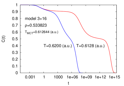
Figure 4: Correlation functions for the model $3+16$: two step relaxation is evident as the temperature is lowered. The exponent parameters are $\lambda_{2}=0.689542$, $\lambda_{1}=0.538201$.

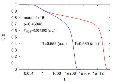
Figure 5: Correlation functions for the model $4+16$: the two step relaxation is practically invisible because of the merging of two nearly logarithmic decays. Indeed, the model parameter exponents are $\lambda_{2}=0.993307$ and $\lambda_{1}=0.992734$ for this model.

3.1 Three step relaxation

Close to the transition point to a $2$RSB phase the correlation function $C(t)$ develops two plateaus for $C(t)=q_{\kappa}$ (with $\kappa=1,2$), with

$$\bar{r}(q_{1})=\bar{r}(q_{2})\ \mbox{and}\ \bar{r}^{\prime}(q_{1})=\bar{r}^{\prime}(q_{2})=0$$ (45)

Near each plateau $q_{k}$ the scaling solution (44) predicts for $C(t)\gtrsim q_{k}$ the power law behavior:

$$C(t)-q_{\kappa}\sim t^{-a_{\kappa}},$$ (46)

with the exponent $0<a_{\kappa}<1/2$ fixed by

$$\lambda_{\kappa}=\frac{\Gamma^{2}(1-a_{\kappa})}{\Gamma(1-2a_{\kappa})},$$ (47)

where

$$\lambda_{\kappa}=\frac{(1-q_{\kappa})^{3}}{2}{\cal M}^{\prime\prime}(q_{\kappa}).$$ (48)

For $C(t)\lesssim q_{\kappa}$ the scaling solution leads the von Schweidler law

$$C(t)-q_{\kappa}\sim-t^{b_{\kappa}}$$ (49)

with the exponent $0<b_{\kappa}<1$ obtained from

$$\lambda_{\kappa}=\frac{\Gamma^{2}(1+b_{\kappa})}{\Gamma(1+2b_{\kappa})}.$$ (50)

In Figs. 4, 5 we show the numerical solution of Eq. (27) close to the dynamical arrest for a system with a $2$RSB phase showing a three steps relaxation and a system displaying a nearly logarithmic decay.

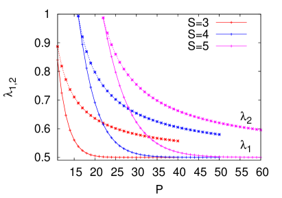
Figure 6: The behavior of the exponent parameters $\lambda_{1}$ (bottom) and $\lambda_{2}$ (top) for different models displaying three step relaxation.

In Fig. 6 we plot the $p$ dependence, at given $s$ for the MCT parameter exponent $\lambda_{1,2}$.

4 Susceptibility spectra

Experimental data are more often available in the frequency domain rather than in the time domain. We show in Figs. 7, 8 the behavior of the susceptibility in cooling procedures towards the $A_{4}$ singularity where the $\beta$ peak, if existing, is most prominent. The two cases are qualitatively quite different. In the case shown in Fig. 7, the $3-16$ model, the onset of a $\beta$ peak is quite tidy. In the $4+16$ case, reported in Fig. 8 no $\beta$ peak is evident not even at very low temperatures and a kind of excess wing appears in its place.

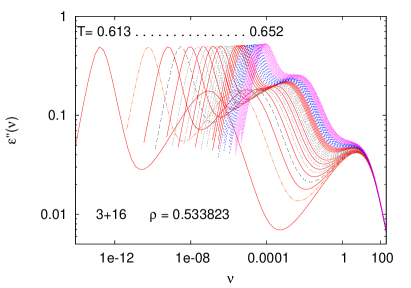
Figure 7: Suceptibility loss for the $3+16$ model in a cooling procedure towards the $A_{4}$ singularity. The $\beta$ peak appears in between $\alpha$ and $\gamma$ peaks as $T$ is decreased.

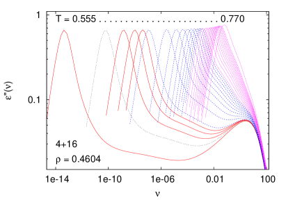
Figure 8: Suceptibility loss for the $4+16$ model in a cooling procedure towards the $A_{4}$ singularity. No full $\beta$ peak develops in cooling.

For what concerns loss spectra, the Mode Coupling scaling next to a $A_{4}$ point in the $\omega$ space, that is next to the minima $\epsilon_{\rm min}^{\kappa}$ of the dynamic susceptibility $\epsilon^{\prime\prime}(\nu)$, becomes [37]:

$$\epsilon^{\prime\prime}(\nu)=\frac{\epsilon_{\rm min}^{\kappa}}{a_{\kappa}+b_{\kappa}}\left[a_{\kappa}\left(\frac{\nu}{\nu_{\rm min}^{\kappa}}\right)^{-b_{\kappa}}+b_{\kappa}\left(\frac{\nu}{\nu_{\rm min}^{\kappa}}\right)^{a_{\kappa}}\right]$$

$$\kappa=1,2$$ (51)

where the height of the minimum scales as $\epsilon_{\rm min}\propto\sqrt{T-T_{\rm mc}}$ and the position of the frequency goes like

$$\nu_{\rm min}^{\kappa}\propto\left(T-T_{\rm mc}\right)^{1/(2a_{\kappa})}$$ (52)

In figure 9 we show an instance of such scaling next to the $A_{4}$ singularity point for the $3+16$ model.

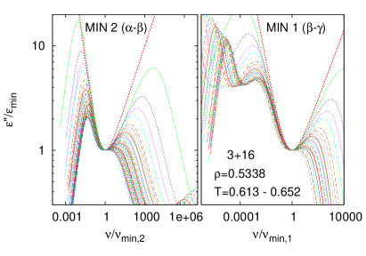
Figure 9: Rescaled loss spectra next to the minima between $\alpha$ and $\beta$ peaks, left, and $\beta$ and $\gamma$ peaks, right.

5 Multi-scale and strechted relaxation

In the mean-field schematic MCT the liquid glass former is homogeneous. Different characteristic relaxation times can occur because of the interplay of different relaxation mechanisms taking place homogeneously in space. Indeed, because of the mean-field nature of MCT [38], position space does not play any role.

In order to have more relaxation times in MCT one has, thus, to resort to a schematic model with a memory kernel more complicated than a simple power of the time autocorrelation function, including at least two parameters, cf. Eq. (8), or including more components, that is involving the correlation of different degrees of freedom [20].

For instance, a $F_{2}$ theory [39, 40] displays dynamic arrest at a certain fold singularity $A_{2}$, denoted by the mode coupling temperature $T_{\rm mc}$ but the relaxation is Debye (a simple exponential in the time domain).

A $F_{12}$ theory [41, 42] colors the $\alpha$ relaxation to something that can be interpreted, i.e., numerically interpolated, as a stretched Kohlrausch-Williams-Watts exponential. The link is provided by setting a correspondence between the $b$ exponent of the von Schweidler law decay from the correlation function plateau and the $\beta_{\rm KWW}$ exponent [37]. However, this only holds next to the plateau (or to a minimum in the loss spectrum), whereas the long time correlation eventually relaxes to zero as an exponential (or a Debye peak in the low frequency domain).

In a two dimensional parameter space $(v_{s},v_{p})$ we observe that enhancing the difference between the powers in the kernel (8) the strechted KWW relaxation (and any related Cole-Cole, or Cole-Davidson or Havriliak-Negami spectrum [43]) is just an artifact of interpolation.

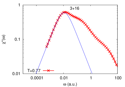
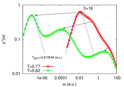
Figure 10: Low frequency Debye relaxation in the $(3,16)$ model. In the supercooled liquid at not very low temperature the beta peak is hidden in the high frequency tail of the alpha relaxation (top), whereas, as temperature is sensitively lowered towards $T_{\rm mc}$ the $\beta$ peak emerges.

For $p\gg s$ we have a $A_{4}$ singularity. In the near proximity to this point dynamic arrest can occur at two different plateaus, each one with its critical slowing down exponents $a_{1,2}$, $b_{1,2}$, and characteristic temperature scalings of the relaxation time $\tau_{1,2}\propto(T-T_{c})^{\gamma_{1,2}}$. Both relaxations are well separated in time, and in frequency, where a minimum of ${\chi(\omega)^{\prime\prime}}$ corresponds to each plateau in $\phi(t)$, cf. Fig. 10. The low frequency susceptibility peaks are, however, clearly Debye. In the time domain this means that, apart from the approach to/decay from the plateaus, the relaxation is exponential.

As we measure correlations and spectra a bit further away from the $A_{4}$ point, though, the two relaxations mix yielding a very well interpolated stretched exponential as shown in Fig. 11.

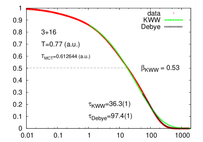
Figure 11: Instance of a very good stretched exponential interpolation of pure two exponentials in the $(3,16)$ model.

6 Conclusions

In this work we have shown how some features of secondary process observed in the relaxation of glass and glassy systems can be captured by a simple schematic model. The model, known as the Spherical $s+p$ Spin Glass model, is a mean field model whose static and dynamics properties can be worked out analytically. In particular its relaxation dynamics is described by the MCT equation with a non-linear memory kernel sum of the a $s-1$ and $p-1$ power. Depending on the value of $s$ and $p$ different scenarios are possible. Secondary processes are observed for $s$ large enough and $p\gg s$. Here we have focused on the properties of the model, connection with experiments will be addressed in a future work.

Eventually we comment of the possibility of describing hierarchies of apart secondary processes, both with discrete or continuous time-scale separation. Though the discrimination of such phenomena is actually rather difficult in experiments, different versions of the present $s+p$ models might straightforwardly account for them [28].

Further work on non-equilibrium dynamics and aging in $s+p$ models with secondary processes is currently in preparation.

Acknowledgments — The research leading to these results has received funding from the People Programme (Marie Curie Actions) of the European Union’s Seventh Framework Programme FP7/2007-2013/ under REA grant agreement no. 290038 - NETADIS project, from the European Research Council through ERC grant agreement no. 247328 - CriPherasy project, and from the Italian MIUR under the Basic Research Investigation Fund FIRB2008 program, grant No. RBFR08M3P4, and under the PRIN2010 program, grant code 2010HXAW77-008. AC acknowledge financial support from European Research Council through ERC grant agreement no. 247328

References

- [1] G. Johari, M. Goldstein, Viscous liquids and the glass transition. III. secondary relaxations in aliphatic alcohols and other nonrigid molecules, J. Chem. Phys.55 (1971) 4245.
- [2] K. Ngai., M. Paluch, Classification of secondary relaxation in glass-formers based on dynamic properties, J. Chem. Phys. 120 (2004) 857.
- [3] A. Döß, M. Paluch, H. Sillescu, G. Hinze, From strong to fragile glass formers: Secondary relaxation in polyalcohols, Phys. Rev. Lett. 88 (2002) 095701.
- [4] P. Lunkenheimer, A. Loidl, Dielectric spectroscopy of glass-forming materials: alpha-relaxation and excess wing, Chem. Phys. 284 (2002) 205.
- [5] S. Kastner, M. Köhler, Y. Goncharov, P. Lunkenheimer, A. Loidl, High-frequency dynamics of type b glass formers investigated by broadbanddielectric spectroscopy, J. of Non-Cryst. Solids 357 (2011) 510–514.
- [6] T. Blochowicz, E. Rössler, Beta relaxation versus high frequency wing in the dielectric spectra of a binary molecular glass former, Phys. Rev. Lett. 92 (2004) 225701.
- [7] T. Blochowicz, S. A. Lusceac, P. Gutfreund, S. Schramm, B. Stühn, Two glass transitions and secondary relaxations of methyltetrahydrofuran in a binary mixture, J. Phys. Chem. B 115 (2011) 1623–1637.
- [8] D. Prevosto, K. Kessairi, S. Capaccioli, M. Lucchesi, P. A. Rolla, Excess wing and johari-goldstein relaxation in binary mixtures of glass formers, Philos. Mag. 87 (2007) 643–650.
- [9] S. Capaccioli, K. Kessairi, M. S. Thayyil, D. Prevosto, M. Lucchesi, The johari-goldstein beta-relaxation of glass-forming binary mixtures, J. of Non-cryst. Solids 357 (2011) 251–257.
- [10] P. Köhler, M. Lunkenheimer, Y. Goncharov, R. Wehn, L. A., Glassy dynamics in mono-, di- and tri-propylene glycol: From the - to the fast -relaxation, J. of Non-Cryst. Solids 356 (2010) 529–534.
- [11] K. Ngai, Relaxation and Diffusion in Complex Systems, Springer, 2011.
- [12] R. Brand, P. Lunkenheimer, U. Schneider, A. Loidl, Is there an excess wing in the dielectric loss of plastic crystals?, Phys. Rev. Lett. 82 (1999) 1951.
- [13] P. Lunkenheimer, R. Wehn, T. Riegger, A. Loidl, Excess wing in the dielectric loss of glass formers: further evidence for a beta-relaxation, J. Non-Cryst. Solids 336 (2002) 307–310.
- [14] J. Wong, C. Angell, Glass: Structure by Spectroscopy, Dekker, New York, 1974.
- [15] K. Ngai, An extended coupling model description of the evolution of dynamics with time in supercooled liquids and ionic conductors, J. Phys. Condens. Matter 15 (2003) S1107.
- [16] H. Z. Cummins, Dynamics-of supercooled liquid: excess wings, ss peaks, and rotation-translation coupling, J. Phys.: Condens. Matter 17 (2005) 1457.
- [17] W. Götze, M. Sperl, Nearly logarithmic decay of correlations in glass-forming liquids, Phys. Rev. Lett. 92 (2004) 105701.
- [18] J. Stevenson, P. Wolynes, A universal origin for secondary relaxations in supercooled liquids and structural glasses, Nat. Phys. 6 (2010) 62.
- [19] J. Wiedersich, T. Blochowicz, S. Benkhof, A. Kudlik, N. Surotsev, C. Tschirwitz, V. Novikov, E. Rössler, Fast and slow relaxation processes in glasses, J. Phys.: Condens. Matter 11 (1999) A147.
- [20] L. Sjögreen, Diffusion of impurities in a dense fluid near the glass transition, Phys. Rev. A 33 (1986) 1254.
- [21] W. Götze, L. Sjögreen, relaxation near glass transition singularities, J. Phys.: Condens. Matter 1 (1989) 4183.
- [22] L. Leuzzi, T. M. Nieuwenhuizen, Thermodynamics of the glassy state, Taylor & Francis, 2007.
- [23] A. Crisanti, L. Leuzzi, Spherical spin-glass model: An exactly solvable model for glass to spin-glass transition, Phys. Rev. Lett. 93 (2004) 217203.
- [24] A. Crisanti, L. Leuzzi, Spherical spin-glass model: An analytically solvable model with a glass-to-glass transition, Phys. Rev. B 73 (2006) 014412.
- [25] L. Leuzzi, Static and dynamic glass-glass transitions: A mean-field study, Philos. Mag. 88 (2008) 4015–4023.
- [26] A. Crisanti, L. Leuzzi, Amorphous-amorphous transition and the two-step replica symmetry breaking phase, Phys. Rev. B 76 (2007) 184417.
- [27] A. Crisanti, L. Leuzzi, T. Rizzo, The Complexity of the Spherical -spin spin glass model, revisited, Eur. Phys. J. B 36 (2003) 129–136.
- [28] A. Crisanti, L. Leuzzi, Equilibrium Dynamics of Spin-Glass Systems, Phys. Rev. B 75 (2007) 144301.
- [29] V. Krakoviack, Comment on “spherical spin-glass model: An analytically solvable model with a glass-to-glass transition”, Phys. Rev. B 76 (2007) 136401.
- [30] A. Crisanti, H. Sommers, The spherical -spin interaction spin-glass model - the statics, Z. Phys. B 87 (1992) 341.
- [31] A. Crisanti, L. Leuzzi, Reply to “comment on ‘spherical spin-glass model: An analytically solvable model with a glass-to-glass transition’ ”, Phys. Rev. B 76 (2007) 136402.
- [32] P. C. Martin, E. Siggia, H. Rose, Statistical dynamics of classical systems, Phys. Rev. A 8 (1973) 423.
- [33] C. De Dominicis, Dynamics as a substitute for replicas in systems with quenched random impurities, Phys. Rev. B 18 (1978) 4913.
- [34] A. Crisanti, Long time limit of equilibrium glassy dynamics and replica calculation, Nucl. Phys. B 796 (2008) 425–456.
- [35] A. Crisanti, H. Horner, H. Sommers, The spherical -spin interaction spin-glass model - the dynamics, Z. Phys. B 92 (1993) 257.
- [36] J.-P. Bouchaud, L. Cugliandolo, J. Kurchan, M. Mézard, Mode-coupling approximations, glass theory and disordered systems, Physica A 226 (1996) 243.
- [37] W. Götze, Complex Dynamics of Glass-Forming Liquids: A Mode-Coupling Theory, Oxford University Press (Oxord, UK), 2009.
- [38] A. Andreanov, G. Biroli, J.-P. Bouchaud, Mode coupling as a landau theory of the glass transition, Europhys. Lett. 88 (2009) 16001.
- [39] E. Leutheusser, Dynamical model of the liquid-glass transition, Phys. Rev. A 29 (1984) 2765.
- [40] U. Bengtzelius, W. Götze, A. Sjölander, Dynamics of supercooled liquids and the glass transition, J. Phys. C 17 (1984) 5915.
- [41] W. G. Götze, Some aspects of phase transitions described by the self consistent current relaxation theory, Z. Phys. B 56 (1984) 139–154.
- [42] T. R. Kirkpatrick, D. Thirumalai, Mean-field soft-spin Potts glass model: Statics and dynamics, Phys. Rev. B 37 (1988) 5342.
- [43] E. Donth, The Glass Transition, Springer (Berlin), 2001.