Vortex hair on AdS black holes

Abstract

We analyse vortex hair for charged rotating asymptotically AdS black holes in the abelian Higgs model. We give analytical and numerical arguments to show how the vortex interacts with the horizon of the black hole, and how the solution extends to the boundary. The solution is very close to the corresponding asymptotically flat vortex, once one transforms to a frame that is non-rotating at the boundary. We show that there is a Meissner effect for extremal black holes, with the vortex flux being expelled from sufficiently small black holes. The phase transition is shown to be first order in the presence of rotation, but second order without rotation. We comment on applications to holography.

1 Introduction

That black holes have no hair is a long-standing dictum of classical general relativity nohair , one whose content is highly contingent upon assumed conditions. Although the original no-hair theorems were more about limiting charges a black hole could carry, they have come to be taken more widely as meaning black holes cannot support nontrivial fields on their event horizon. This outlook is supported by the original no hair theorems for gauge fields and scalars ChaseAdler , which placed what were regarded as eminently reasonable conditions on matter fields. In the intervening years, however, it has become clear that these conditions are not only too restrictive nohair2 , but in fact there are many situations of physical interest in which black holes can support nontrivial field configurations. Most of these are concerned with asymptotically flat space times otherhair whose hair falls off sufficiently rapidly at large distances from the black hole, though there are examples of nonsingular cosmological solutions with time dependence coshair , or indeed scalar condensates around Kerr black holes Kerrscalar .

Topological defects form an interesting class of alternative examples of black hole hair outside of the asymptotically flat class. Both domain walls and cosmic strings Vilenkin , topologically stable objects with a nontrivial quantum-field-theoretic vacuum structure, can have significant gravitational influence, and were originally expected to be antipathetic to black holes, in part because of the problem of how to have the associated fields end on the event horizon, but also because of the strong global gravitational impact of the black hole. Domain walls provide a ‘mirror’ to spacetime (effectively compactifying space IpS ) and cosmic strings yield a conical deficit that generates a gravitational lens Vilenkin2 . It is now known that both can “pierce” the black hole EGS ; AGK : in the former case, the field theoretic wall provides a smooth transition between mirror images of the northern hemisphere of the C-metric, whereas in the latter case a smooth version of the Aryal-Ford-Vilenkin metric AFV represents a black hole with a conical deficit through its poles. The original solution AGK has been generalized in a number of ways to include vortices ending on black holes RGMH , charged black holes CCESa ; BEG , dilatonic black holes ROG , rotating black holes GB ; GKW , and asymptotically dS GMdS and AdS black holes VH ; DGM1 . Fields typically terminate on the event horizon or, in the case of extremal black holes, be expelled from the horizon if the width of the string is comparable to the size of the black hole.

Most recently, the rotating black hole has been subject to a thorough study GKW , which analysis corrected earlier work that had a flawed ansatz GB . There is now a detailed understanding of how the core fields of a vortex accommodate the rotation of asymptotically flat black holes and their associated ‘electric’ field generation. The vortex cuts out a local co-rotating deficit azimuthal angle, which leads to some novel features, shifting the ergosphere of the black hole and altering the innermost stable circular orbit (ISCO). As with charged black holes, flux expulsion can indeed take place under certain circumstances. However unlike the charged case the phase transition is of first order and numerical evidence suggests that the flux-expelled solution is not dynamically stable.

Here, we investigate the impact of a negative cosmological constant on the problem of a vortex piercing a black hole. Specifically, we obtain vortex solutions for an Abelian Higgs model minimally coupled to Einstein gravity in four dimensions with a negative cosmological constant. We obtain both approximate and numerical vortex solutions to the field equations of the Abelian Higgs model in the background of a Kerr-Newman-AdS black hole. We find that as the AdS length, $\ell$, becomes comparable to the size of the vortex, the core of the vortex increasingly narrows and the fields exhibit asymptotic power-law falloff instead of exponential. We find that the Meissner effect, observed previously for extremal Kerr and Reissner-Nordstrom black holes, persists here as well, and is first order if there is non-zero rotation but is otherwise 2nd order. We find that the flux can pierce the horizon provided the AdS length is sufficiently large, and numerically obtain the critical radius for the transition from piercing to expulsion.

Our work may have interesting astrophysical implications. It has long been known Wald ; Expulsion1 that spinning black holes tend to expel magnetic fields in a continuous way as the black hole is spun up. Indeed, it has been argued that all stationary, axisymmetric magnetic fields are expelled from the Kerr horizon in the extremal limit Expulsion2 . Since a Killing vector in the vacuum spacetime can act as a vector potential for a Maxwell test field, as the hole is ‘spun up’ toward extremality, the component of the magnetic field normal to the horizon approaches zero, and so the flux lines are expelled (a phenomenon that also occurs for black strings and $p$-branes Expulsion3 ). This Meissner-like effect could quench the power of astrophysical jets, since the magnetic fields need to pierce the horizon to extract rotational energy from the black hole, though it has been recently argued Penna that split-monopole magnetic fields may continue to power black hole jets, with the fields becoming entirely radial near the horizon, avoiding expulsion. In contrast to this we find (as for the asymptotically flat case GKW ) in the Abelian Higgs model that for large AdS black holes the vortex pierces the event horizon, whereas flux is expelled if the black hole is sufficiently small.

From a holographic perspective, a vortex in the bulk has an interpretation as a defect in the the dual CFT VH ; Dias:2013bwa , corresponding in the dual superfluid to heavy pointlike excitations around which the phase of the condensate winds. We comment briefly at the end of our paper on a holographic interpretation of our results.

2 Abelian Higgs model for a cosmic string

The abelian Higgs model is the canonical toy model for a cosmic string, as it has the simplest action with the requisite vacuum structure to allow a vortex to form. We write the action as

$$S=\int d^{4}x\sqrt{-g}\left[D_{\mu}\Phi^{\dagger}D^{\mu}\Phi-{\textstyle{\frac{1}{4}}}{\tilde{F}}_{\mu\nu}{\tilde{F}}^{\mu\nu}-{\textstyle{\frac{1}{4}}}\lambda(\Phi^{\dagger}\Phi-\eta^{2})^{2}\right]\,,$$ (1)

where $\Phi$ is the Higgs field, and $A_{\mu}$ the U(1) gauge boson with field strength ${\tilde{F}}_{\mu\nu}$. As per usual, we rewrite the field content as:

$$\Phi(x^{\alpha}) = \eta X(x^{\alpha})e^{i\chi(x^{\alpha})}\,,$$ (2)

$$A_{\mu}(x^{\alpha}) = \frac{1}{e}\left[P_{\mu}(x^{\alpha})-\nabla_{\mu}\chi(x^{\alpha})\right]\,.$$ (3)

These fields extract the physical degrees of freedom of the broken symmetric phase, with $X$ representing the residual massive Higgs field, and $P_{\mu}$ the massive vector boson. The gauge degree of freedom, $\chi$, is explicitly subtracted, although any non-integrable phase factors have a physical interpretation as a vortex.

In terms of these new variables, the equations of motion are

$$\nabla_{\mu}\nabla^{\mu}X-P_{\mu}P^{\mu}X+\frac{\lambda\eta^{2}}{2}X(X^{2}-1) = 0\,,$$ (4)

$$\nabla_{\mu}F^{\mu\nu}+2e^{2}\eta^{2}X^{2}P^{\nu} = 0\,.$$ (5)

Because we have not set $G\equiv 1$, we still have the freedom to fix the units of energy, or $\eta$. We therefore choose to set $\sqrt{\lambda}\eta=1$, effectively stating our Higgs field has order unity mass. For further use we also introduce the Bogomol’nyi parameter Bog :

$$\beta=\lambda/2e^{2}\,,$$ (6)

indicating the gauge field has mass of order $1/\sqrt{\beta}$. Alternately, we can rescale the dimensionful parameters $t$ and $r$ in the equations of motion: $t\to\sqrt{\lambda}\eta t$, etc. and their corresponding gauge field components $P_{t}\to P_{t}/\sqrt{\lambda}\eta$ – note $P_{\phi}$ remains unrescaled however.

A straight static vortex solution will then have the Higgs profile, $X_{NO}$, dependent on a single radial variable, $R$ say, and the gauge field will have a single angular component, $P_{\phi}=P_{NO}(R)$, where in flat spacetime $X_{NO}$ and $P_{NO}$ satisfy the Nielsen-Olesen equations NO

$$X_{NO}^{\prime\prime}+\frac{X_{NO}^{\prime}}{R} =\frac{P_{NO}^{2}X_{NO}}{R^{2}}+\frac{1}{2}X_{NO}(X_{NO}^{2}-1)\,,$$ (7)

$$P_{NO}^{\prime\prime}-\frac{P_{NO}^{\prime}}{R} =\frac{X_{NO}^{2}P_{NO}}{\beta}\,.$$

The profiles of the $X_{NO}$ and $P_{NO}$ fields are highly localized around $R=0$, and represent a Higgs core in which the U(1) symmetry is restored with (in this case) a unit of magnetic flux threading through. Higher winding strings can be obtained by replacing $P_{NO}\to NP_{NO}$, although these are unstable to splitting for $\beta>1$.

Since we are interested in vortices in an anti-de Sitter black hole background, for future reference we now discuss the vortex solution in the pure AdS geometry:

$$ds^{2} =\Bigl{(}1+\frac{r^{2}}{\ell^{2}}\Bigr{)}dt^{2}-\frac{dr^{2}}{\left(1+\frac{r^{2}}{\ell^{2}}\right)}-r^{2}d\theta^{2}-r^{2}\sin^{2}\!\theta d\phi^{2}$$ (8)

$$=\frac{\ell^{2}+R^{2}}{\ell^{2}(1-Z^{2})}dt^{2}-\frac{\ell^{2}+R^{2}}{(1-Z^{2})^{2}}dZ^{2}-\frac{\ell^{2}dR^{2}}{\ell^{2}+R^{2}}-R^{2}d\phi^{2}\,.$$

By writing the AdS metric in this second, cylindrical, form we can see that if we align the vortex in the $\{R,\phi\}$ plane, the equations of motion will be independent of $Z$, and hence our vortex can once again be represented by a set of ordinary differential equations:

$$\left(1+\frac{R^{2}}{\ell^{2}}\right)P_{0}^{\prime\prime}+\left(\frac{2R^{2}}{\ell^{2}}-1\right)\frac{P_{0}^{\prime}}{R} =\frac{X_{0}^{2}P_{0}}{\beta}\,,$$ (9)

$$\left(1+\frac{R^{2}}{\ell^{2}}\right)X_{0}^{\prime\prime}+\left(\frac{4R}{\ell^{2}}+\frac{1}{R}\right)X_{0}^{\prime}-\frac{P_{0}^{2}X_{0}}{R^{2}}-\frac{1}{2}X_{0}(X_{0}^{2}-1) =0\,.$$

As $R\to 0$, the additional terms dependent on the AdS background drop away, and we have a very similar field structure on axis to the Nielsen-Olesen vortex. For $R\gtrsim\ell$ however, the functions are modified, and the asymptotic fall-off of the fields becomes power law rather than exponential.

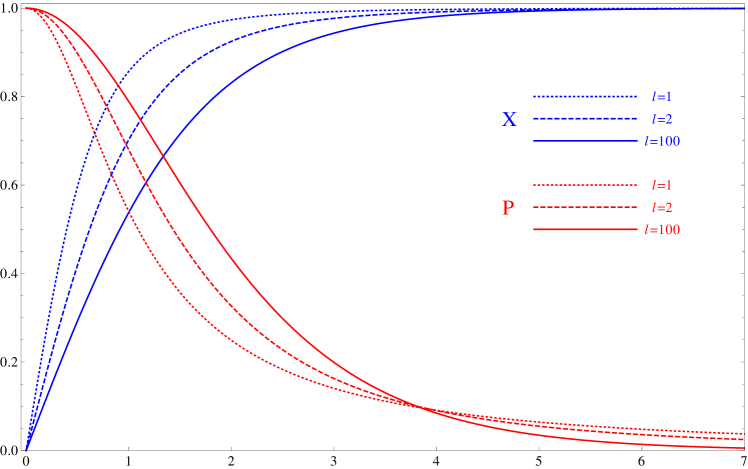
Figure 1: AdS-NO vortex: The values of $X$ and $P$ for the AdS NO vortex are depicted as functions of $R$.

In figure 1 we show the Higgs and gauge profiles for the AdS vortex. At large $\ell$, the profile is essentially the same as the pure NO-vortex. However as $\ell$ approaches the scale of the vortex, the core is seen to narrow, and the power law fall-off becomes more apparent. Although we can formally integrate these equations for $\ell\lesssim 1$, it is unclear that such solutions with our boundary conditions are physically relevant, as the false vacuum $X=0$ becomes stable for Compton wavelengths above the AdS scale BF .

3 Vortices in Kerr-AdS: Analytics

Although the full exact solution of a vortex in a black hole background must be found numerically, there are two ways in which we can gain insight into the system analytically. The first is by construction of an approximate solution, and the second is the case of extremal black holes in which we can prove the existence (or not) of a piercing solution on the event horizon.

We start by writing down the charged rotating black hole solution CarterCMP

$$ds^{2}=\frac{\Delta}{\Sigma}\left[dt-\frac{a\sin^{2}\!\theta}{\Xi}d\phi\right]^{2}-\frac{\Sigma}{\Delta}dr^{2}-\frac{\Sigma}{S}d\theta^{2}-\frac{S\sin^{2}\!\theta}{\Sigma}\left[adt-\frac{r^{2}+a^{2}}{\Xi}d\phi\right]^{2}\,,$$ (10)

where

$$\Sigma = r^{2}+a^{2}\cos^{2}\!\theta\,,\quad\Xi=1-\frac{a^{2}}{\ell^{2}}\,,\quad S=1-\frac{a^{2}}{\ell^{2}}\cos^{2}\!\theta\,,$$

$$\Delta = (r^{2}+a^{2})\Bigl{(}1+\frac{r^{2}}{\ell^{2}}\Bigr{)}-2mr+q^{2}\,,$$ (11)

and the $U(1)$ potential is

$$A=-\frac{qr}{\Sigma}\left(dt-\frac{a\sin^{2}\!\theta}{\Xi}d\phi\right)\,.$$ (12)

The mass $M$, the charge $\mathcal{Q}$, and the angular momentum $J$ are related to the parameters $m$, $q$, and $a$ as follows:

$$GM=\frac{m}{\Xi^{2}}\,,\quad G\mathcal{Q}=\frac{q}{\Xi}\,,\quad GJ=\frac{am}{\Xi^{2}}\,.$$ (13)

The ergosphere is located at $\Delta=a^{2}S\sin^{2}\theta$, and the horizon at $\Delta=0$. For large $\ell$, the horizon is just slightly perturbed from its Kerr-Newman value. As $\ell$ decreases, the horizon radius drops, and for small $\ell$ asymptotes to $m^{1/3}\ell^{2/3}$ (or $\sqrt{q\ell}$ for nonzero charge). We see therefore that for smaller values of $\ell$, the fact that $m\gg 1$ is no guarantee that the horizon radius must also be similarly large in general. However, as we have already remarked, we do not expect $\ell\lesssim 1$ to be physically relevant. Therefore in any analytic approximation, we will assume $\ell>1$.

Before moving to the vortex equations and analytic results, it is worth remarking on the behaviour of the horizon radius in a little more detail, and how this depends on $\ell$. This is most succinctly captured by the extremal horizon radius, when $\Delta=\Delta^{\prime}=0$, which implies

$$r_{+}=\frac{\ell}{\sqrt{6}}\left[\left(\left(1+\frac{a^{2}}{\ell^{2}}\right)^{2}+12\left(\frac{a^{2}+q^{2}}{\ell^{2}}\right)\right)^{1/2}-\left(1+\frac{a^{2}}{\ell^{2}}\right)\right]^{1/2}\,.$$ (14)

We see therefore that $r_{+}(a,q,\ell)<\sqrt{a^{2}+q^{2}}$, the Kerr-Newman value. Moreover, as $\ell$ drops, it is easy to see that $r_{+}$ also drops, and for $\ell\lesssim 10$ drops quite sharply. Therefore, for the purposes of finding an approximate solution for the vortex functions, which typically assumes the black hole is large, we must consider $\ell\gtrsim 10$, and for considerations of flux expulsion, which typically happens for small black holes, we would expect any argument to be sensitive to the value of $\ell$.

To find the vortex equations, we must consider not only the $X$ and $P_{\phi}$ functions, but also a nonzero $P_{t}$:

$$0 = \Delta X_{,rr}+\Delta^{\prime}X_{,r}+SX_{,\theta\theta}+\cot\theta\Bigl{(}S+\frac{2a^{2}}{\ell^{2}}\sin^{2}\theta\Bigr{)}X_{,\theta}$$ (15)

$$+\Sigma P_{\mu}^{2}X-\frac{\Sigma}{2}X(X^{2}-1)\,,$$

$$\frac{X^{2}}{\beta}P_{t} = \frac{\triangle}{\Sigma}P_{t,rr}+\frac{S}{\Sigma}P_{t,\theta\theta}+\frac{2a\Xi\cot\theta}{\Sigma^{3}}\Bigl{(}\rho^{2}S-\Delta+\frac{a^{2}}{\ell^{2}}\Sigma\sin^{2}\!\theta\Bigr{)}P_{\phi,\theta}$$ (16)

$$-\frac{a\Xi}{\Sigma^{3}}\Bigl{(}2r(Sa^{2}\sin^{2}\!\theta-\Delta)+\Sigma\Delta^{\prime}\Bigr{)}P_{\phi,r}$$

$$+\frac{\cot\theta}{\Sigma^{3}}\left(S\bigl{(}\rho^{4}+a^{4}\sin^{4}\!\theta\bigr{)}-2a^{2}\sin^{2}\!\theta\Bigl{(}\Delta-\frac{\rho^{2}\Sigma}{\ell^{2}}\Bigr{)}\right)P_{t,\theta}$$

$$-\frac{\sin^{2}\!\theta}{\Sigma^{3}}\Bigl{(}a^{2}\bigl{(}2r\rho^{2}S+\Sigma\Delta^{\prime}\bigr{)}-\frac{2r\rho^{2}\Delta}{\sin^{2}\!\theta}\Bigr{)}P_{t,r}\,,$$

$$\frac{X^{2}}{\beta}P_{\phi} = \frac{\Delta}{\Sigma}P_{\phi,rr}+\frac{S}{\Sigma}P_{\phi,\theta\theta}+\frac{\rho^{2}}{\Sigma^{3}}\bigl{(}2rSa^{2}\sin^{2}\!\theta+\Sigma\Delta^{\prime}-2r\Delta\bigr{)}P_{\phi,r}$$ (17)

$$+\frac{\cot\theta}{\Sigma^{3}}\left(2a^{2}\sin^{2}\!\theta\Bigl{(}\Delta-\frac{a^{2}}{\ell^{2}}\Sigma\sin^{2}\!\theta\Bigr{)}-S\Bigl{(}a^{2}\sin^{2}\!\theta(\rho^{2}-\Sigma)+\rho^{4}\Bigr{)}\right)P_{\phi,\theta}$$

$$+\frac{2\cot\theta a^{3}\sin^{4}\!\theta}{\Xi\Sigma^{3}}\left(\Delta-\rho^{2}\Bigl{(}1+\frac{r^{2}}{\ell^{2}}\Bigr{)}\right)P_{t,\theta}$$

$$+\frac{a\sin^{2}\!\theta}{\Xi\Sigma^{3}}\Bigl{(}2r\bigl{(}\rho^{4}S-\Delta(\Sigma+\rho^{2})\bigr{)}+\rho^{2}\Sigma\Delta^{\prime}\Bigr{)}P_{t,r}\,,$$

where $\rho^{2}=r^{2}+a^{2}$ has been introduced for visual clarity, $\Delta^{\prime}=d\Delta/dr$, and

$$P_{\mu}^{2}=\frac{(\rho^{2}P_{t}+a\Xi P_{\phi})^{2}}{\Sigma\Delta}-\frac{(\Xi P_{\phi}+a\sin^{2}\!\theta P_{t})^{2}}{\Sigma S\sin^{2}\!\theta}\,.$$ (18)

3.1 Approximate solution

As with the original Schwarzschild, Reissner-Nordstrom and Kerr black holes, it is useful to develop an analytic approximate solution. Clearly we expect this to make use of the (possibly AdS) Nielsen Olesen solutions, and to depend on a single function of $r$ and $\theta$.

Consider the function

$$R\equiv\frac{\rho}{\sqrt{\Xi}}\sin\theta\,,$$ (19)

which tends to the Kerr expression $\rho\sin\theta$ as $\ell\to\infty$. Then, assuming that the vortex is much thinner than the black hole horizon radius means that $\rho$ is always much greater than one, and focusing on the core region of the vortex [$R<{\cal O}(10)$] means that $\sin\theta\ll 1$. We can therefore expand the metric functions

$$\Sigma=\rho^{2}\left(1-\frac{a^{2}R^{2}\Xi}{\rho^{4}}\right)\simeq\rho^{2}\,,\quad S=\Xi\left(1+\frac{a^{2}R^{2}}{\ell^{2}\rho^{2}}\right)\simeq\Xi\,,$$ (20)

and derivatives as

$$\frac{\partial~{}}{\partial r} = \frac{Rr}{\rho^{2}}\frac{d~{}}{dR}\,,\qquad\frac{\partial~{}}{\partial\theta}=\frac{\rho}{\sqrt{\Xi}}\left(1-\frac{\Xi R^{2}}{\rho^{2}}\right)^{1/2}\frac{d~{}}{dR}\simeq\frac{\rho}{\sqrt{\Xi}}\frac{d~{}}{dR}\,,$$

$$\Delta\frac{\partial^{2}~{}}{\partial r^{2}}+S\frac{\partial^{2}~{}}{\partial\theta^{2}} = \left[S\Bigl{(}\frac{\rho^{2}}{\Xi}-R^{2}\Bigr{)}+\frac{\Delta R^{2}r^{2}}{\rho^{4}}\right]\frac{d^{2}~{}}{dR^{2}}+\Bigl{(}\frac{\Delta a^{2}}{\rho^{4}}-S\Bigr{)}R\frac{d~{}}{dR}$$

$$\simeq \rho^{2}\Bigl{(}1+\frac{\Delta R^{2}}{\rho^{4}}\Bigr{)}\frac{d^{2}~{}}{dR^{2}}\,,$$

to leading order in $R/\rho$. This already leads to significant simplification of several of the terms in (15)-(17). Then a little experimentation suggests the following approximate functions

$$X\simeq X_{0}(R)\,,\quad P_{\phi}\simeq P_{0}(R)\,,\quad P_{t}\simeq\frac{a}{\rho^{2}}\Bigl{(}\frac{\Delta}{\rho^{2}}-\Xi\Bigr{)}P_{0}(R)\,,$$ (22)

which to leading order give the approximate equations:

$$0 =\left(1+\frac{\Delta R^{2}}{\rho^{4}}\right)X_{0}^{\prime\prime}+\left(1+\frac{4R^{2}}{\ell^{2}}\right)\frac{X_{0}^{\prime}}{R}-\frac{P_{0}^{2}X_{0}}{R^{2}}-\frac{X_{0}}{2}(X_{0}^{2}-1)\,,$$ (23)

$$\frac{X_{0}^{2}}{\beta}P_{0} =\left(1+\frac{\Delta R^{2}}{\rho^{4}}\right)P_{0}^{\prime\prime}-\left(1+\frac{\left(2\Delta-r\Delta^{\prime}\right)R^{2}}{\rho^{4}}\right)\frac{P_{0}^{\prime}}{R}\,.$$

Away from the horizon, $\Delta\sim\rho^{4}/\ell^{2}$ to leading order, and we recover the AdS Nielsen-Olesen equations (9). However retaining the $R^{2}/\ell^{2}$ terms is perhaps misleading, as we require $\ell>{\cal O}(10)$ in order for the horizon radius of an extremal black hole not to be too small. We also see that on (or near) the horizon, the ${\cal O}(R^{2}/\ell^{2})$ corrections to the Nielsen-Olesen equations fail to have the precise AdS form. This implies that while we can use the analytic approximation to good effect away from the black hole, near the horizon we would expect corrections to our solution at order ${\cal O}(\ell^{-2})$.

Note that because of the behaviour of $\Delta$ at large $r$, the approximation for $P_{t}$ in (22) actually becomes proportional to $P_{\phi}$ at large $r$: $P_{t}\sim aP_{\phi}/\ell^{2}$. Our gauge field is thus

$$\textbf{\em P}=P_{\phi}d\phi+P_{t}dt\sim P_{0}(R)\left(d\phi+\frac{a}{\ell^{2}}dt\right)\,,$$ (24)

therefore it would appear that we have an electric field inside our vortex far from the black hole. In fact, this is simply an artifact of the Boyer-Lindquist style coordinates we have used in (10), which asymptote AdS₄ in a rotating frame with angular momentum $\Omega_{\infty}=a/\ell^{2}$ GPP . One may remove this rotation by introducing new variables

$$\varphi=\phi+\frac{a}{l^{2}}t\,,\quad T=t\,.$$ (25)

It is then easy to check that P in (22) now reads

$$\textbf{\em P}=P_{0}(R)\Bigl{(}d\varphi-\frac{a(2mr-q^{2})}{\rho^{4}}dT\Bigr{)}\,.$$ (26)

The $P_{T}$ component is now negative definite and falls off appropriately at large $r$. The form of this solution is now identical to that used in GKW .

Figure 2 shows a comparison of this pseudo-analytic approximation with a numerically obtained solution for an extremal low mass lowish $\ell$ black hole. We take the values $m=3,\ell=20,q=0$, and with $a\simeq 2.939$ at its extremal value in order to draw a parallel with the plot in GKW . What is clearly shown is that the approximation is extremely good almost everywhere, the only slight discrepancy appearing near the event horizon – as expected given the structure of the corrections to the approximation there.

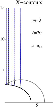
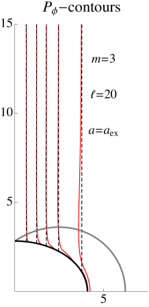
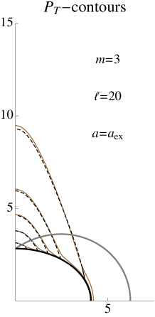
Figure 2: Approximate vs. numerical solution: In each case the numerical solution is shown in solid colour, and the approximation in dashed black. Contours of $0.1-0.9$ (in steps of $0.2$) of the range of each field are shown. From left to right: The Higgs field in blue, the $P_{\phi}$ field in red, and $P_{T}$ (the component with respect to the nonrotating frame at infinity) in brown. For $P_{T}$, we show contours of $0.1-0.9$ of the maximal negative value, which is attained on the poles of the horizon. The outer grey curve represents the boundary of the ergosphere.

3.2 Extremal black holes

The extremal horizon exhibits a Meissner effect for the cosmic string, in which if the black hole becomes too ‘small’ the cosmic string magnetic flux is expelled from the black hole, and the horizon remains in the false vacuum. For both Reissner-Nordstrom BEG and Kerr GKW black holes, the existence of this phase transition has been proven analytically, as well as demonstrated numerically. The Reissner-Nordstrom transition is second order, corresponding to a continuous change in the order parameter (the magnitude of the Higgs field) between piercing and expelling solutions. For the Kerr black hole however, the phase transition was first order, corresponding to a discontinuous change in the value of the gradient of the zeroth component of the gauge field between piercing and expelling solutions.

We will now argue for the existence of a Meissner effect in the AdS-Kerr-Newman black holes; the Kerr-Newman situation follows from taking the large-$\ell$ limit. Begin by defining new variables $P$ and $Q$:

$$SP=\Xi P_{\phi}+a\sin^{2}\!\theta P_{t}\,,\quad(r-r_{+})Q=\rho^{2}P_{t}+a\Xi P_{\phi}\,,$$ (27)

where the factors have been chosen so that the horizon equations are clearly identifiable, and the range of $P$ is $P\in[0,1]$. The field equations (15)-(16) become

$$0 = \frac{\Delta}{\Sigma}X,_{rr}+\frac{\Delta^{\prime}}{\Sigma}X,_{r}+\frac{1}{\Sigma\sin\theta}\Bigl{(}S\sin\theta X,_{\theta}\Bigr{)},_{\theta}$$ (28)

$$+\left(\frac{(r-r_{+})^{2}Q^{2}}{\Sigma\,\Delta}-\frac{P^{2}}{\Sigma\,S\,\sin^{2}\theta}\right)X-\frac{X}{2}(X^{2}-1),$$

$$\frac{X^{2}P}{\beta} = \frac{\Delta}{\Sigma}P,_{rr}+\frac{S}{\Sigma}P,_{\theta\theta}+\frac{\Sigma\Delta^{\prime}-2r\Delta}{\Sigma^{2}}P_{,r}+\frac{\cot\theta}{\Sigma}\Bigl{(}4\frac{a^{2}}{l^{2}}\sin^{2}\!\theta-\frac{S}{\Sigma}\bigl{(}\Sigma-2a^{2}\sin^{2}\!\theta\bigr{)}\Bigr{)}P,_{\theta}$$ (29)

$$+\frac{2a\sin^{2}\theta}{\Sigma^{2}}\left((r-r_{+})\left(rQ_{,r}-\cot\theta\,Q_{,\theta}-Q\right)+aP\Bigl{(}1-\frac{r^{2}}{l^{2}}\Bigr{)}+rQ\right)\,,$$

$$\frac{X^{2}Q}{\beta} = \frac{\Delta}{\Sigma}\frac{\left[(r-r_{+})Q\right]_{,rr}}{(r-r_{+})}+\frac{S}{\Sigma}Q_{,\theta\theta}+\frac{\cot\theta}{\Sigma^{2}}(2a^{2}\sin^{2}\theta(1+\frac{r^{2}}{\ell^{2}})+S\,\Sigma)Q_{,\theta}$$ (30)

$$+\frac{2\Delta}{\Sigma^{2}}\left(\frac{a}{(r-r_{+})}(rSP_{,r}-S\cot\theta P_{,\theta}-(2-S)P)-rQ_{,r}-\frac{r_{+}Q}{(r-r_{+})}\right)\,,$$

which in the extremal limit and on the horizon reduce to

$$\left(S\sin\theta X^{\prime}\right)^{\prime} = X\sin\theta\left[\frac{SP^{2}}{\sin^{2}\theta}-\frac{2Q^{2}}{\Delta^{\prime\prime}_{+}}-\frac{\Sigma_{+}}{2}(1-X^{2})\right],$$ (31)

$$\left(\frac{S^{2}P^{\prime}}{\Sigma_{+}\sin\theta}\right)^{\prime} = PS\sin\theta\left[\frac{X^{2}}{\beta\sin^{2}\theta}-\frac{2a^{2}}{\Sigma_{+}^{2}}\left(1-\frac{r_{+}^{2}}{\ell^{2}}\right)\right]-\frac{2ar_{+}SQ\sin\theta}{\Sigma_{+}^{2}}\,,$$ (32)

$$\left(\frac{S\sin\theta Q^{\prime}}{\Sigma_{+}}\right)^{\prime} = \frac{X^{2}Q}{\beta}\sin\theta\,,$$ (33)

where a prime now denotes $d/d\theta$, and the “$+$” subscript indicates the function is evaluated at $r=r_{+}$, given by (14). Note that unlike the vacuum Kerr case, in which $r_{+}=a$, there is no simple factorization of $\Sigma_{+}$ leading to a clean $\theta$-dependence in these equations.

Note that if $a=0$, $Q\equiv 0$, and $S\equiv 1$ and our system of horizon equations reduces precisely to the Reissner-Nordstrom horizon equations studied in BEG . Therefore we expect essentially the same analytic arguments to hold here (which is the case as we shall see below). Further, since $Q$ vanishes, we expect a second order phase transition governed by the continuous order parameter $X$. On the other hand, if $a\neq 0$, $Q$ is nonzero in the bulk of the spacetime and so we must examine the full system of horizon equations.

Let us look first at the behaviour of the horizon function $Q$, as this will give us the order of the phase transition. For a piercing solution, $X$ is nontrivial on the horizon. Hence

$$S\beta\sin\theta Q^{\prime}(\theta)=\Sigma_{+}\int_{0}^{\theta}{X^{2}Q\sin\theta}d\theta\,,$$ (34)

upon integrating (33). We can easily see this cannot be true unless $Q\equiv 0$. Evaluating (34) at the first point at which $Q^{\prime}=0$ tells us that $\int_{0}^{\theta}{X^{2}Q\sin\theta}=0$, but $Q$ is either positive and increasing on this range, or negative and decreasing: in either case, the integrand is positive or negative definite, thus cannot be zero. Therefore $Q\equiv 0$ for a piercing solution. On the other hand, an expelling solution has $X\equiv 0$, with $P_{\phi}=1$, hence

$$P=\frac{\Xi\Sigma_{+}}{\rho_{+}^{2}S}\,,\qquad Q\equiv-\frac{2ar_{+}\Xi}{\rho_{+}^{2}}\,.$$ (35)

Given that $Q$ changes in a discontinuous fashion, we see that the phase transition is first order for nonzero $a$.

It is clear that a flux expelling solution to the horizon system of equations (31)-(33) can exist. However to prove flux expulsion happens, this solution must be extendable to a bulk solution. To demonstrate this, we follow the argument of BEG . If flux is expelled, $X\equiv 0$ on the horizon, and must become nonzero and positive a small distance from the horizon, implying $(\Delta X_{,r})_{,r}>0$ just outside the horizon. Referring to (28), we see therefore that

$$(S\sin\theta X_{,\theta})_{,\theta}+\frac{(r_{+}^{2}+a^{2}\cos^{2}\theta)X}{2}\sin\theta<\frac{SP^{2}}{\sin\theta}X<\frac{SX}{\sin\theta}$$ (36)

is required if a flux expelling solution is to exist. Integrating this inequality on $[\theta_{0},\pi/2]$ gives

$$S\sin\theta_{0}X_{,\theta_{0}}>\int_{\theta_{0}}^{\pi/2}\left(\frac{(r_{+}^{2}+a^{2}\cos^{2}\theta)\sin\theta}{2}-\frac{S}{\sin\theta}\right)Xd\theta\,.$$ (37)

Defining $\alpha$ so that $\Sigma_{+}\sin^{2}\alpha/S=2$, by taking $\theta_{0}>\alpha$ we can bound this integral from below using $X(\theta)>X(\theta_{0})$. We can also bound the derivative of $X$ by $X_{,\theta_{0}}<\frac{X(\theta_{0})-X(\alpha)}{\theta_{0}-\alpha}<\frac{X(\theta_{0})}{\theta_{0}-\alpha}$, leading to

$$S\sin\theta_{0}\frac{X(\theta_{0})}{\theta_{0}-\alpha}>S\sin\theta_{0}X_{,\theta_{0}}>X(\theta_{0})\int_{\theta_{0}}^{\pi/2}\left(\frac{(r_{+}^{2}+a^{2}\cos^{2}\theta)\sin\theta}{2}-\frac{S}{\sin\theta}\right)d\theta\,,$$ (38)

which implies

$$\frac{({\theta_{0}-\alpha})}{S(\theta_{0})\sin\theta_{0}}\left(\frac{r_{+}^{2}\cos\theta_{0}}{2}+\frac{a^{2}\cos^{3}\theta_{0}}{6}+\Xi\log\tan\Bigl{(}\frac{\theta_{0}}{2}\Bigr{)}-\frac{a^{2}}{l^{2}}\cos\theta_{0}\right)<1$$ (39)

on the interval $[\alpha,\pi/2]$. If this inequality is violated, then we cannot have flux expulsion, and the vortex must pierce the black hole. Note, if $a=0$, then (39) is independent of $\ell$, and reduces to the previously explored Reissner-Nordstrom relation BEG , giving the same upper bound on the horizon radius for flux expulsion of $\sqrt{8.5}$. For $a\neq 0$, we must explore the $\{a,\ell\}$ phase plane (having ensured that a solution $\alpha$ exists) to determine the upper bound on the horizon radius. Clearly if $\ell$ drops too low, we require a large charge to allow for a solution to $\alpha$. Hence for a given $q$, we expect a minimal value of $\ell$ for this upper bound to exist. This is shown most clearly for $q=0$, in figure 3.

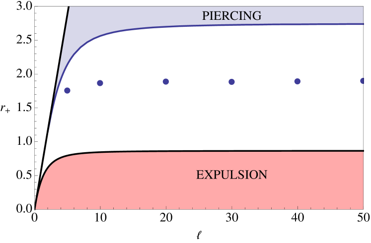
Figure 3: Meissner effect: An illustration of the analytic bounds on the critical horizon radius for the Meissner effect for $q=0$. In the shaded regions, the vortex should either pierce the horizon, or be expelled as indicated. The critical radius therefore lies between these two bounds. For sufficiently low $\ell$, flux is always expelled. Numerically obtained transition radii are indicated. The solid $r_{+}=\ell/\sqrt{3}$ line on the left indicates the $a=\ell$ singular limit.

To argue that a Meissner effect should exist for sufficiently low horizon scales, we assume a piercing solution to (31)-(33) exists, in which $X$ and $P$ will have nontrivial profiles symmetric around $\theta=\pi/2$, with $X$ maximised and $P$ minimised (at least for large $\ell$ or small $a<q$) at $\pi/2$. If $a=0$, the argument of BEG can be used to deduce that for $r_{+}\lesssim 0.7$ the flux must be expelled, and this argument can be extended to include small $a$ (see appendix). For $q=0$, or dominant $a$, an alternate argument must be used. At large $\ell$, $P$ is minimised at $\pi/2$, which implies a constraint on $r_{+}$ given by (writing $X_{m}=X(\pi/2)$):

$$P^{\prime\prime}\left(\frac{\pi}{2}\right) =P\left(\frac{X_{m}^{2}r_{+}^{2}}{\beta}-\frac{2a^{2}}{r_{+}^{2}}\Bigl{(}1-\frac{r_{+}^{2}}{\ell^{2}}\Bigr{)}\right)\geq 0\;\;\;\Rightarrow\;\;\;r_{+}^{4}+2r_{+}^{2}\frac{a^{2}\beta}{\ell^{2}}>2a^{2}\beta\,.$$ (40)

However, for low values of $\ell$, we cannot show that $P$ is minimised at $\pi/2$, and indeed scrutiny of piercing solutions near the phase transition indicates a tiny modulation in $P$. What we can say however, is that $P$ has at most one additional turning point on $[0,\pi/2]$, as the source term on the RHS of (32) is monotonically decreasing on $[0,\pi/2]$, hence $S^{2}P^{\prime}/\Sigma_{+}\sin\theta$ has at most one turning point where $X^{2}\Sigma_{+}^{2}=2a^{2}\beta\sin^{2}\theta(1-r_{+}^{2}/\ell^{2})$.

Suppose therefore that we are at low $\ell$ and $P$ has such a turning point on $[0,\pi/2]$. Now consider $S^{2}/\Sigma_{+}\sin\theta$; the derivative

$$\left(\frac{S^{2}}{\Sigma_{+}\sin\theta}\right)^{\prime}=-\frac{S\cot\theta}{\Sigma_{+}^{2}\sin\theta}\left[(r_{+}^{2}+a^{2})\Xi-3a^{2}\Bigl{(}1+\frac{r_{+}^{2}}{\ell^{2}}\Bigr{)}\sin^{2}\theta+\frac{a^{4}}{\ell^{2}}\sin^{4}\theta\right]$$ (41)

has a zero at $\theta_{0}$, where

$$\frac{a^{2}}{\ell^{2}}\sin^{2}\theta_{0}=\frac{3}{2}\left(1+\frac{r_{+}^{2}}{\ell^{2}}\right)-\frac{1}{2}\sqrt{9\left(1+\frac{r_{+}^{2}}{\ell^{2}}\right)^{2}-4\Xi\frac{r_{+}^{2}+a^{2}}{\ell^{2}}}\,.$$ (42)

For $q=0$, $\sin\theta_{0}\in[0,\sqrt{2/3}]$, as $\ell$ ranges from $a$ to $\infty$, whereas the node in $P$ only switches on for lower $\ell$, and initially appears at $\pi/2$. Therefore at $\theta_{0}$ we expect $S^{2}P^{\prime}/\Sigma_{+}\sin\theta>0$, and hence

$$(r_{+}^{2}+a^{2}\cos^{2}\theta_{0})^{2}>X^{2}(\theta_{0})\Sigma_{+}^{2}(\theta_{0})>2a^{2}\beta\sin^{2}\theta_{0}\Bigl{(}1-\frac{r_{+}^{2}}{\ell^{2}}\Bigr{)}\,.$$ (43)

Thus, if this equality is not satisfied at $\theta_{0}$, we deduce that a piercing solution is not possible, and expulsion must occur. Figure 3 shows this lower bound for $q=0$.

The full details of the phase transition must be determined numerically, and figure 3 shows the numerically obtained critical horizon radius as a function of $\ell$ for $q=0$ together with the analytic lower and upper bounds on $r_{+,crit}$. We discuss the phase transition further in section 5.

4 Numerical solution

In order to obtain numerical solutions of the vortex equations (15)-(17), which form an elliptic system, we follow references AGK and GKW , employing a gradient flow technique on a two-dimensional polar grid. Briefly, this method introduces a fictitious time variable, with the ‘rate of change’ of our functions being proportional to the actual elliptic equations we wish to solve:

$$\dot{Y}^{i}=\Delta Y^{i}+F^{i}(\bf{Y},\nabla\bf{Y})\,,$$ (44)

where $\Delta^{i}$ represents a second order (linear) elliptic operator and $F$ is a (possibly nonlinear) function of the variables $Y^{i}$ and their gradients, such that the RHS is our system of elliptic equations. We now have a diffusion problem, and solutions to this new equation eventually “relax” to a steady state, in which the variables are no longer changing with each time step, and the solutions $Y^{i}$ satisfy our elliptic equations. The only subtlety with the given set-up is that our elliptic system has one boundary (the event horizon) on which our equations become parabolic. This was discussed in detail in AGK , with the result that on each grid update, we update the event horizon, using the horizon equations, and fixing

$$P_{t}=-\frac{a\Xi P_{\phi}}{r_{+}^{2}+a^{2}}\,$$ (45)

on the horizon, which is mandated by finiteness of the energy-momentum tensor.

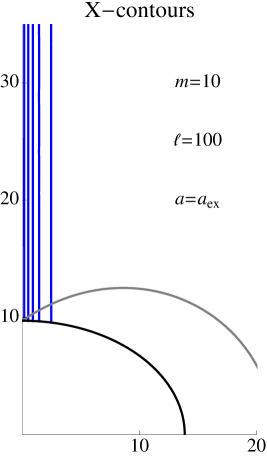
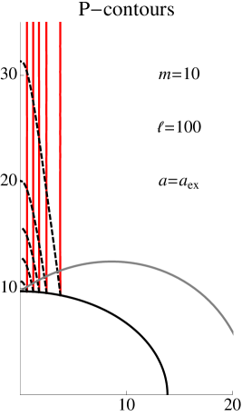
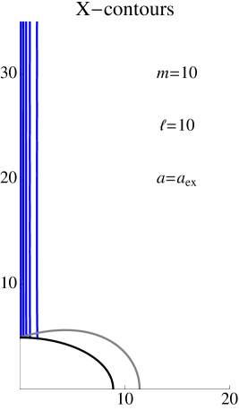
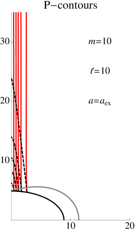
Figure 4: AdS-Kerr vortex: A depiction of the numerical solution for the AdS-Kerr vortex for an extremal uncharged rotating black hole. The upper plots have $\ell=100$, the lower plots $\ell=10$. In each case, the contours of the Higgs field are shown on the left in blue ($X=0.1-0.9$ in steps of $0.2$), and on the right, the angular component of the gauge field, $P_{\varphi}$ in red (with the same contour steps as for $X$), and $P_{T}$ in dashed black with contours of $0.1-0.9$ of $P_{T,min}=-0.0519,-0.116$ for the $\ell=100$ and $\ell=10$ cases respectively.

As an initial condition for the integration, we use the approximate solutions for the functions $X$, $P_{\phi}$ and $P_{t}$ given in equations (22), where we obtain the forms for $P_{0}(R)$ and $X_{0}(R)$ by numerically integrating (9) on a one-dimensional grid. The approximate solution is accurate to order $r^{-2}$, thus we choose our outer boundary to be sufficiently far from the horizon that our analytic approximation is extremely accurate near this outer radial boundary, which is not updated in our code. On axis we impose the standard vortex boundary conditions, ($X=0$, $P_{\phi}=1$) while leaving $P_{t}$ to relax by continuity. As pointed out in GKW , the fact that $P_{t}$ is not restricted can be understood by noting that there is a dyonic degree of freedom that is introduced into the solution due to the presence of the black hole.

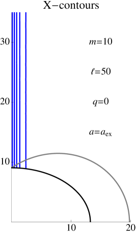
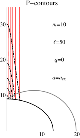
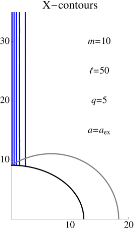
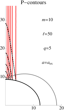
Figure 5: AdS-Kerr-Newman vortex: Numerical solutions for the AdS-Kerr-Newman vortex with $\ell=50$ and $q=0$, (upper) and $q=5$ (lower) with the same contour conventions as for figure 4, with $P_{T,min}=-0.0569$ for $q=0$, and $P_{T,min}=-0.0563$ for $q=5$.

Figures 4 and 5 show a selection of the solutions obtained from the integration method above which highlight the effects of the parameters $\ell$ and $q$ on the rotating black hole vortex. In all plots, we have chosen to illustrate the solution by plotting contour lines for each field of $0.1-0.9$ of the full range of the field in steps of $0.2$. Thus, for the $X$ and $P_{\phi}$ fields, we have shown the $0.1,0.3,0.5,0.7$, and $0.9$ contours, but for the $P_{T}$ field (note – this is the gauge field component with respect to a non-rotating frame at infinity) the maximally negative value of $P_{T}$ is attained on the horizon at the poles. The numerical values of these contours therefore vary from plot to plot. The actual value of $P_{T,min}$ is given in the captions.

Figure 4 shows the vortex solution for the case of $\ell=100$ and $\ell=10$ respectively, at the extremal limit with the charge parameter $q$ set to zero. The solution away from the extremal limit is similar (see GKW ), the main difference being that the actual numerical values of the $P_{T}$ contours are lower. For $\ell=100$, the plots are almost indistinguishable from the vacuum Kerr vortex solution analysed in GKW , however, for $\ell=10$, the effect of the cosmological constant can be easily seen. Comparing the figures, one notes that dropping the value of $\ell$ strongly impacts the size of both the black hole horizon as well as the vortex, causing the vortex width to tighten, the $P_{T}$ fields to shrink closer to the horizon, which itself shrinks significantly.

Figure 5 then demonstrates the effect of adding a non-zero charge to the AdS-Kerr vortex. As can be seen, this does not significantly impact the vortex, and appears to merely shift the horizon and ergosphere inwards, while slightly causing the $P_{T}$ contour lines to creep closer to the horizon, as is expected since the rotation parameter $a=a_{ex}$ will be lower with the charged black hole at the same mass.

5 Discussion

We have examined the behaviour and interactions of vortices with asymptotically AdS charged and rotating black holes. We first obtained an approximate solution to the abelian Higgs Model in the background of a Kerr-Newman AdS black hole, and showed that the Nielsen-Olesen equations retain their AdS form up to corrections of order $R^{2}/\ell^{2}$. Consequently we found that our approximation was extremely good everywhere except near the event horizon as expected. The comparison illustrated in figure 2 shows that the actual solution has a stronger expulsion of flux than the approximation. Upon transforming to a frame that is non-rotating at the boundary, the form of our solution is very close to its asymptotically flat counterpart.

For extremal black holes we explored the existence of a Meissner effect with the cosmic string flux being expelled from the black hole at small horizon radii (although one should be cautious about the stability of such small black holes CarDias ). We presented analytic arguments to show that such a phase transition exists, showing that in the presence of rotation it is a first order transition. We numerically explored the phase space to confirm this expectation, and figure 6 shows the numerical results for the phase transition at several values of $\ell$ and $\beta$. The existence of the first order transition is confirmed, and the effect of $\ell$ is to lower the critical value of $r_{+}$ at which the transition occurs. This is also reflected in a drop of both analytic bounds for expulsion and piercing of the vortex. We also notice that the value of the order parameter ($X(\pi/2)$) rises with decreasing $\ell$, seen in the right plot of figure 6. The left plot of figure 6 shows the effect of changing $\beta$, and is similar to the corresponding plot for the vacuum Kerr solution in GKW . However the effect of changing $\beta$ is far more pronounced at the relatively low value of $\ell=10$ illustrated. Note that, unlike pure Kerr, the plots do not extend to $r_{+}^{-1}\to 0$: there is an upper limit on the angular momentum, and hence horizon radius.

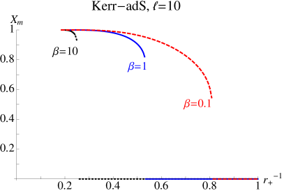
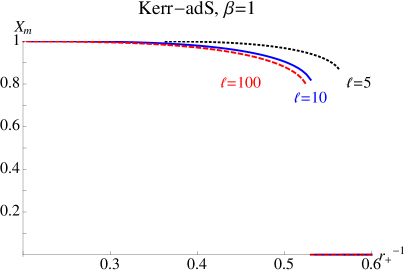
Figure 6: Flux expulsion behavior: Plots illustrating features of the flux expulsion phase transition on the event horizon of the black hole. The maximal value of the Higgs field $X_{m}=X(\pi/2)$ is shown as a function of $r_{+}^{-1}$ for varying $\beta$ (left) and $\ell$ (right).

The numerical integrations are considerably more sensitive with the addition of the cosmological constant, mainly because an additional scale has been added which causes the vortex to contract, as well as the black hole. Unfortunately this has prevented us from investigating the small-$\ell$ case in significant detail. This is the region of interest for a holographic interpretation of our results, though our solution would only be relevant in the IR as it does not have the requisite boundary conditions.

Vortices in the bulk can be interpreted as defects in the dual CFT VH ; Dias:2013bwa , where in the IR they are heavy pointlike excitations in a superfluid around which the phase of the condensate winds. A vortex must have a core radius since the vanishing of the condensate at its location is energetically costly and so must happen over some finite region. A recent study Dias:2013bwa of vortices with planar black holes has indicated that their IR physics can be understood from the viewpoint of a defect or boundary CFT Cardy:2004hm . A study of holographic superconductivity in the context of (topologically spherical) rotating black holes Sonner found that the superconducting state in the dual theory (for certain choices of parameters) can be destroyed for sufficiently large rotation. The localization of the condensate depends on the sign of the mass-squared term of the scalar, with a droplet/ring-like structure appearing for positive/negative values of this term. The instability towards forming vortex anti-vortex pairs depends on this sign Sonner .

It would be interesting to study these effects further in light of our results. Even without rotation we obtain a Meissner effect, and so very small black holes with expelled flux can exist. Their interpretation in the context of the boundary theory (as well as distinguishing them from the flux-pierced case) remains to be understood, perhaps in terms of the absence of a mass gap for the flux-expelled case.

Appendix A Lower bound argument

Following BEG , assume a piercing solution exists, then (31) and (32) have smooth solutions for $X$ and $P$ in which $X$ increases from zero at the poles to a maximum, $X_{m}$ at the equator, and $P$ decreases from $1$ at the poles to a minimum, $P_{m}$, at the equator. Evaluating (31) and (32) at the equator gives the relations:

$$X^{\prime\prime}\left(\frac{\pi}{2}\right) =X_{m}\left[P^{2}_{m}+\frac{r_{+}^{2}}{2}\left(X^{2}_{m}-1\right)\right]\leq 0\ \Rightarrow\ P_{m}^{2}\leq\frac{r_{+}^{2}}{2}\left(1-X^{2}_{m}\right)\leq\frac{r_{+}^{2}}{2}\,,$$ (46)

$$P^{\prime\prime}\left(\frac{\pi}{2}\right) =P_{m}\left[\frac{X_{m}^{2}r_{+}^{2}}{\beta}-\frac{2a^{2}}{r_{+}^{2}}\left(1-\frac{r_{+}^{2}}{\ell^{2}}\right)\right]\geq 0\ \Rightarrow\ r_{+}^{4}\geq X_{m}^{2}r_{+}^{4}\geq 2a^{2}\beta\Bigl{(}1-\frac{r_{+}^{2}}{\ell^{2}}\Bigr{)}\,.\quad$$ (47)

Since $P\leq 1$, the first relation gives no new information unless $r_{+}<\sqrt{2}$, so we will assume this from now on. The second relation clearly gives no information if $a=0$; however, for nonzero $a$ and sufficiently small $q$, the bound (47) is violated at sufficiently low $\ell$, or indeed if $q<a\lesssim 0.6$ for all $\ell$.

If $a$ is sufficiently small that (47) does not give useful information, then we can bound $r_{+}$ by a generalisation of the argument in BEG . Assuming a piercing solution, (47) bounds $P^{\prime\prime}(\pi/2)$ above by:

$$P^{\prime\prime}\left(\frac{\pi}{2}\right)\leq\frac{r_{+}}{\sqrt{2}}\left[\frac{X_{m}^{2}r_{+}^{2}}{\beta}-\frac{2a^{2}}{r_{+}^{2}}\Bigl{(}1-\frac{r_{+}^{2}}{\ell^{2}}\Bigr{)}\right]\sqrt{1-X_{m}^{2}}\leq\frac{\sqrt{2}r_{+}^{3}}{3\sqrt{3}\beta}\left(1-\frac{2a^{2}\beta}{r_{+}^{4}}\Bigl{(}1-\frac{r_{+}^{2}}{\ell^{2}}\Bigr{)}\right)^{3/2}\!\!\!,$$ (48)

where we use (46), and maximise over $X_{m}$ in the second inequality.

To get a lower bound on $P^{\prime\prime}$ we use $P^{\prime\prime}(\pi/2)\geq-P^{\prime}(\theta_{0})/(\pi/2-\theta_{0})$, where $\theta_{0}$ is where $P^{\prime}$ is maximally negative, (32) giving:

$$P^{\prime}\left(\theta_{0}\right)=-\frac{P\tan\theta}{\beta}\frac{\Sigma_{+}^{2}X^{2}-2a^{2}\beta\sin^{2}\theta\left(1-r_{+}^{2}/\ell^{2}\right)}{S(\Sigma_{+}-2a^{2}\sin^{2}\theta)-4\Sigma_{+}(a^{2}/\ell^{2})\sin^{2}\theta}\Bigg{|}_{\theta=\theta_{0}}\,.$$ (49)

Thus

$$\left|P^{\prime}\left(\theta_{0}\right)\right| \leq\frac{P(\theta_{0})\tan\theta_{0}}{\beta}\frac{\Sigma_{+}^{2}(\theta_{0})-2a^{2}\beta\sin^{2}\theta_{0}\left(1-r_{+}^{2}/\ell^{2}\right)}{S(\theta_{0})(\Sigma_{+}(\theta_{0})-2a^{2}\sin^{2}\theta_{0})-4\Sigma_{+}(\theta_{0})(a^{2}/\ell^{2})\sin^{2}\theta_{0}}$$ (50)

$$\leq\frac{\bigl{(}r_{+}^{4}-2a^{2}\beta\left(1-r_{+}^{2}/\ell^{2}\right)\bigr{)}\,\tan\theta_{0}}{\bigl{(}r_{+}^{2}(1-4a^{2}/\ell^{2})-2a^{2}\bigr{)}\,\beta}\,.$$

Clearly for this bound to be meaningful, we also require $r_{+}^{2}(1-4a^{2}/\ell^{2})>2a^{2}$, so we will assume this going forward. We therefore have that

$$\frac{\pi}{2}-\theta_{0}<\cot\theta_{0}\leq\frac{r_{+}^{4}-2a^{2}\beta\left(1-r_{+}^{2}/\ell^{2}\right)}{\bigl{(}r_{+}^{2}(1-4a^{2}/\ell^{2})-2a^{2}\bigr{)}\,\beta\,|P_{0}^{\prime}|}\,,$$ (51)

meanwhile

$$1-\frac{\pi}{2}|P_{0}^{\prime}|<P_{m}<\frac{r_{+}}{\sqrt{2}}\qquad\Rightarrow\qquad|P_{0}^{\prime}|>\frac{2}{\pi}\Bigl{(}1-\frac{r_{+}}{\sqrt{2}}\Bigr{)}\,,$$ (52)

giving

$$P^{\prime\prime}\left(\frac{\pi}{2}\right)\geq\frac{|P_{0}^{\prime}|}{\pi/2-\theta_{0}}\geq\beta|P_{0}^{\prime}|^{2}\frac{r_{+}^{2}(1-4a^{2}/\ell^{2})-2a^{2}}{r_{+}^{4}-2a^{2}\beta\left(1-r_{+}^{2}/\ell^{2}\right)}\,.$$ (53)

Folding this in with the upper bound on $P^{\prime\prime}(\pi/2)$, we see that for a piercing solution to exist the following inequality must hold:

$$\frac{6\sqrt{6}\beta^{2}}{\pi^{2}}\Bigl{(}1-\frac{r_{+}}{\sqrt{2}}\Bigr{)}^{2}\left(1-\frac{2a^{2}\beta}{r_{+}^{4}}\Bigl{(}1-\frac{r_{+}^{2}}{\ell^{2}}\Bigr{)}\right)^{-5/2}\frac{r_{+}^{2}(1-4a^{2}/\ell^{2})-2a^{2}}{r_{+}^{7}}<1\,,$$ (54)

with $2>r_{+}^{2}>2a^{2}/(1-4a^{2}/\ell^{2})$ and $r_{+}^{4}+2a^{2}r_{+}^{2}/\ell^{2}>2a^{2}\beta$. The former of these bounds places a stronger constraint on $a$, but in fact the constraint (54) breaks down before even this is violated. Since the value of $r_{+}$ satisfying (54) is quite low (just less than one), the relation gives no useful information once $a$ gives a significant contribution to $r_{+}$. For large $\ell$, this happens around $a\sim 0.7$, but for $\ell$ of order unity or below, this happens at a much lower value ($\sim 0.3$ for $\ell=1$). We illustrate the running of this lower bound with $a$ in figure 7.

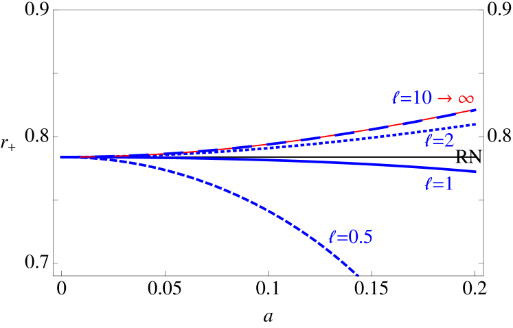
Figure 7: Expulsion bound: An illustration of the running of the lower bound with $a$. The bound is plotted for $\ell=0.5,1,2,10,\infty$ as labeled. For $\ell>5$, the curve changes very little, as can be seen by the infinite $\ell$ curve depicted by a thin red line. The value at $a=0$ is the RN value obtained in BEG , and is shown as the horizontal solid black line.

The actual value of this bound is less important than the fact it exists, which then implies the existence of a phase transition on the event horizon and flux expulsion.

References

- (1) P. T. Chrusciel, ‘No hair’ theorems: Folklore, conjectures, results, Contemp. Math. 170, 23 (1994). [gr-qc/9402032].
-
(2)
J. E. Chase,
Event Horizons in Static Scalar-Vacuum Space-Times,
Com. Math. Phys. 19 276–288 (1970).
S. L. Adler and R. B. Pearson, ‘No Hair’ Theorems for the Abelian Higgs and Goldstone Models, Phys. Rev. D18, 2798 (1978). - (3) J. D. Bekenstein, Black hole hair: 25 - years after, In Moscow 1996, 2nd International A.D. Sakharov Conference on physics 216-219 [gr-qc/9605059].
-
(4)
P. Bizon,
Colored black holes,
Phys. Rev. Lett. 64, 2844 (1990).
H. Luckock and I. Moss, Black Holes Have Skyrmion Hair, Phys. Lett. B176, 341 (1986).
K. -M. Lee, V. P. Nair and E. J. Weinberg, Black holes in magnetic monopoles, Phys. Rev. D45, 2751 (1992) [hep-th/9112008]. -
(5)
T. Jacobson,
Primordial black hole evolution in tensor scalar cosmology,
Phys. Rev. Lett. 83, 2699 (1999)
[astro-ph/9905303].
S. Chadburn and R. Gregory, Time dependent black holes and scalar hair, [arXiv:1304.6287 [gr-qc]].
E. Abdalla, N. Afshordi, M. Fontanini, D. C. Guariento and E. Papantonopoulos, Cosmological black holes from self-gravitating fields, [arXiv:1312.3682 [gr-qc]]. -
(6)
S. Hod,
Stationary Scalar Clouds Around Rotating Black Holes,
Phys. Rev. D 86, 104026 (2012)
[Erratum-ibid. D 86, 129902 (2012)]
[arXiv:1211.3202 [gr-qc]].
C. A. R. Herdeiro and E. Radu, Kerr black holes with scalar hair, Phys. Rev. Lett. 112, 221101 (2014) [arXiv:1403.2757 [gr-qc]]. -
(7)
A. Vilenkin,
Cosmic Strings and Domain Walls,
Phys. Rept. 121, 263 (1985).
A. Vilenkin and E. P. S. Shellard, Cosmic Strings and other Topological Defects. Cambridge University Press, Cambridge, England, 1994. -
(8)
J. Ipser and P. Sikivie,
The Gravitationally Repulsive Domain Wall,
Phys. Rev. D30, 712 (1984).
G. W. Gibbons, Global structure of supergravity domain wall space-times, Nucl. Phys. B394, 3 (1993). - (9) A. Vilenkin, Gravitational Field of Vacuum Domain Walls and Strings, Phys. Rev. D23, 852 (1981).
- (10) R. Emparan, R. Gregory and C. Santos, Black holes on thick branes, Phys. Rev. D63, 104022 (2001) [hep-th/0012100].
- (11) A. Achucarro, R. Gregory, and K. Kuijken, Abelian Higgs hair for black holes, Phys. Rev. D52 (1995) 5729–5742, [gr-qc/9505039].
- (12) W. Kinnersley and M. Walker, Uniformly accelerating charged mass in general relativity, Phys. Rev. D2, 1359 (1970).
- (13) M. Aryal, L. Ford, and A. Vilenkin, Cosmic strings and black holes, Phys. Rev. D34 (1986) 2263.
-
(14)
R. Gregory and M. Hindmarsh,
Smooth metrics for snapping strings,
Phys. Rev. D52 (1995) 5598–5605,
[gr-qc/9506054].
D. M. Eardley, G. T. Horowitz, D. A. Kastor and J. H. Traschen, Breaking cosmic strings without monopoles, Phys. Rev. Lett. 75, 3390 (1995) [gr-qc/9506041].
S. W. Hawking and S. F. Ross, Pair production of black holes on cosmic strings, Phys. Rev. Lett. 75, 3382 (1995) [gr-qc/9506020].
R. Emparan, Pair creation of black holes joined by cosmic strings, Phys. Rev. Lett. 75, 3386 (1995) [gr-qc/9506025].
A. Achucarro and R. Gregory, Selection rules for splitting strings, Phys. Rev. Lett. 79, 1972 (1997) [hep-th/9705001]. -
(15)
A. Chamblin, J. Ashbourn-Chamblin, R. Emparan, and A. Sornborger,
Can extreme black holes have (long) Abelian Higgs hair?,
Phys. Rev. D58 (1998) 124014,
[gr-qc/9706004].
A. Chamblin, J. Ashbourn-Chamblin, R. Emparan, and A. Sornborger, Abelian Higgs hair for extreme black holes and selection rules for snapping strings, Phys. Rev. Lett. 80 (1998) 4378–4381, [gr-qc/9706032].
F. Bonjour and R. Gregory, Comment on ‘Abelian Higgs hair for extremal black holes and selection rules for snapping strings’, Phys. Rev. Lett. 81 (1998) 5034, [hep-th/9809029]. - (16) F. Bonjour, R. Emparan, and R. Gregory, Vortices and extreme black holes: The Question of flux expulsion, Phys. Rev. D59 (1999) 084022, [gr-qc/9810061].
-
(17)
R. Moderski and M. Rogatko,
Abelian Higgs hair for electrically charged dilaton black holes,
Phys. Rev. D58, 124016 (1998)
[hep-th/9808110].
L. Nakonieczny and M. Rogatko, Abelian-Higgs hair on stationary axisymmetric black hole in Einstein-Maxwell-axion-dilaton gravity, Phys. Rev. D88, 084039 (2013) [arXiv:1310.5929 [hep-th]]. - (18) A. Ghezelbash and R. B. Mann, Abelian Higgs hair for rotating and charged black holes, Phys. Rev. D65 (2002) 124022, [hep-th/0110001].
- (19) R. Gregory, D. Kubiznak and D. Wills, Rotating black hole hair, JHEP 1306, 023 (2013) [arXiv:1303.0519 [gr-qc]].
- (20) A. Ghezelbash and R. Mann, Vortices in de Sitter space-times, Phys.Lett. B537 (2002) 329–339, [hep-th/0203003].
- (21) M. H. Dehghani, A. M. Ghezelbash and R. B. Mann, Vortex holography, Nucl. Phys. B625, 389 (2002) [hep-th/0105134].
- (22) M. Dehghani, A. Ghezelbash, and R. B. Mann, Abelian Higgs hair for AdS-Schwarzschild black hole, Phys. Rev. D65 (2002) 044010, [hep-th/0107224].
- (23) R. Wald, Black hole in a uniform magnetic field, Phys. Rev. D10 (1974) 1680–1685.
- (24) A. R. King, J. P. Lasota, and W. Kundt, Black holes and magnetic fields, Phys. Rev. D12 3037 (1975).
-
(25)
J. Bičák and L. Dvořák,
Stationary electromagnetic fields around black holes.
II. General solutions and the fields of some special sources
near a Kerr black hole
General Relativity and Gravitation, 7 959 (1976)
J. Bičák and L. Dvořák, Stationary electromagnetic fields around black holes. III. General solutions and the fields of current loops near the Reissner-Nordström black hole, Phys. Rev. D22 2933 (1980). - (26) A. Chamblin, R. Emparan and G. W. Gibbons, Superconducting p-branes and extremal black holes, Phys. Rev. D58, 084009 (1998), [arXiv:9806017 [hep-th]].
- (27) R. F. Penna, The Black Hole Meissner Effect and Blandford-Znajek Jets, [arXiv:1403.0938 [astro-ph.HE]].
- (28) O. J. C. Dias, G. T. Horowitz, N. Iqbal and J. E. Santos, Vortices in holographic superfluids and superconductors as conformal defects [arXiv:1311.3673 [hep-th]].
- (29) E. B. Bogomolnyi, The stability of classical solutions, Sov. J. Nucl. Phys. 24 (1976) 449.
- (30) H. B. Nielsen and P. Olesen, Vortex Line Models for Dual Strings, Nucl. Phys. B61 (1973) 45–61.
- (31) P. Breitenlohner and D. Z. Freedman, Stability in Gauged Extended Supergravity, Annals Phys. 144, 249 (1982).
- (32) B. Carter, Hamilton-Jacobi and Schrodinger separable solutions of Einstein’s equations, Commun. Math. Phys. 10, 280 (1968).
- (33) G. W. Gibbons, M. J. Perry and C. N. Pope, The First law of thermodynamics for Kerr-anti-de Sitter black holes, Class. Quant. Grav. 22, 1503 (2005) [hep-th/0408217].
- (34) V. Cardoso and O. J. C. Dias, Small Kerr-anti-de Sitter black holes are unstable, Phys. Rev. D 70, 084011 (2004) [hep-th/0405006].
- (35) J. L. Cardy, Boundary conformal field theory [arXiv:hep-th/0411189].
- (36) J. Sonner, A Rotating Holographic Superconductor, Phys. Rev. D80, 084031 (2009) [arXiv:0903.0627 [hep-th]].