optomechanically induced amplification and perfect transparency in double-cavity optomechanics

Abstract

We study the optomechanically induced amplification and perfect transparency in a double-cavity optomechanical system. We find if two control lasers with appropriate amplitudes and detunings are applied to drive the system, the phenomenon of optomechanically induced amplification for a probe laser can occur. In addition, perfect optomechanically induced transparency phenomenon, which is robust to mechanical dissipation, can be realized by the same type of drive. These results are very important for signal amplification, light storage, fast light and slow light in the quantum information processes.

I Introduction

Cavity optomechanics, exploring the interaction between light fields and mechanical motions, has attracted a lot of attention in the past few years for its potential application in the ultrasensitive detection of tiny mass, force, and displacement A1 ; A2 ; A3 ; A4 . One standard and simplest optomechanical setup is a Fabry-Perot cavity with one end mirror being a micro- or nano-mechanical vibrating object B1 ; B2 ; B3 . Other various optomechanical experimental system are designed and investigated such as silica toroidal optical microresonators C1 ; C2 ; C3 , photonic crystal cavities D1 ; D2 , micromechanical membranes E1 ; E2 , typical optomechanical cavities confining cold atoms f1 ; f2 , superconducting circuits g1 ; g2 , and so on.

Typically, when driving an otomechanical cavity by a red-detuned laser, the mechanical oscillator can be cooled to its quantum ground-state h1 ; h2 ; h3 . Moreover, in this red-detuned regime, some well-known phenomena in atomic ensemble can find their analogy in optomechanical system. Specifically, under a strong driving, normal mode splitting j1 ; j2 (called Autler-Townes effects in atomic physics) can be observed. On the contrary, for a relatively weak driving (much less than the cavity dissipation rate), an electromagnetically induced transparency like phenomenon, called optomechanically induced transparencyL1 ; L2 ; L3 , has been theoretically predict and experimentally verified. This phenomenon can be used to slow down and even stop light signals M1 ; M2 in the long-lived mechanical vibrations. On the other hand, when a driving laser applied on the mechanical blue sideband, the mechanical element of an optomecanical system can be heated, leading to phonon lasing i1 ; i2 ; i3 and probe amplification p1 ; p2 ; N1 ; N2 .

In our previous work, we have investigated coherent perfect transmission and absorption in a double-cavity optomechanical system driven by two pump fields on red mechanical sideband q1 . While in this paper, we study the optomechanically induced amplification and perfect transparency in the same system driven under a different type of drive. We find that if driving the double-cavity optomechanical system by a red sideband laser from one side and a blue sideband one from the other side and appropriately manipulating the amplitudes of them, optomechanically induced amplification phenomenon can occur for a nearly resonant weak signal field (probe field). In addition, by adjusting the control fields, an interesting perfect optomechanically induced transparency (with transmission coefficient rigorously equal to 1) can be realized under the same type of drive. When this perfect transmission occur, quantum coherence process due to the double-driving can totally suppress the decoherence due to the dissipation of mechanical resonator. This double-driving device could be used to realize signal quantum amplifier, quantum switch, quantum memory and so on.

The rest of this paper is organized as follows. In Section II, we introduce the double-cavity optomechanical model, obtain the equations of motion for the mechanical resonator and the two cavity modes, and solve them and obtain the output fields. In Section III, we show how to realize perfect optomechanically induced transparency even though with big mechanical decay rate $\gamma_{m}$. In Section IV, we show how to realize optomechanically induced amplification about the weak signal field (probe field), meanwhile, the system holds below the phonon lasing threshold. And the conclusions are given in the Section V.

II Model and Equations

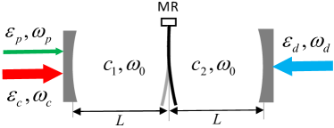
Figure 1: (Color online) A double-cavity optomechanical system with a mechanical resonator (MR) inserted between two fixed mirrors. The two cavities have identical cavity lengths $L$ and mode frequencies $\omega_{0}$ in the absence of radiation pressure. Coupling field and driving field with frequencies $\omega_{c},\omega_{d}$ and amplitudes $\varepsilon_{c},\varepsilon_{d}$ respectively, act upon opposite sides of the double-cavity system. The probe field with frequency $\omega_{p}$ and amplitude $\varepsilon_{p}$ is injected into the left optical cavity.

We consider a double-cavity hybrid system with one mechanical resonator (MR) of perfect reflection inserted between two fixed mirrors of partial transmission (see Fig. 1). The MR has an eigen frequency $\omega_{m}$ and a decay rate $\gamma_{m}$ and thus exhibits a mechanical quality factor $Q=\omega_{m}/\gamma_{m}$. Two identical optical cavities of lengths $L$ and frequencies $\omega_{0}$ are got when the MR is at its equilibrium position in the absence of external excitation. We describe the two optical modes, respectively, by annihilation (creation) operators $c_{1}$ ($c_{1}^{\dagger}$) and $c_{2}$ ($c_{2}^{\dagger}$) while the only mechanical mode by $b$ ($b^{\dagger}$). These annihilation and creation operators are restricted by the commutation relation $[c_{i},c_{i}^{\dagger}]=1$ ($i=1,2$) , $[c_{1},c_{2}]=0$, and $[b,b^{\dagger}]=1$. Two coupling fields are used to drive the double-cavity system from either left or right fixed mirrors with their amplitudes denoted by $\varepsilon_{c}=\sqrt{2\kappa\wp_{c}/(\hbar\omega_{c})}$ and $\varepsilon_{d}=\sqrt{2\kappa\wp_{d}/(\hbar\omega_{d})}$ and one probe field is injected into the left optical cavity with amplitude denoted by $\varepsilon_{p}=\sqrt{2\kappa\wp_{p}/(\hbar\omega_{p})}$. Here $\wp_{c}$, $\wp_{d}$ and $\wp_{p}$, are relevant field powers, $\kappa$ is the common decay rate of both cavity modes, and $\omega_{c}$, $\omega_{d}$, and $\omega_{p}$, are relevant field frequencies. Then the total Hamiltonian in the rotating-wave frame of frequency $\omega_{c}+\omega_{d}$ can be written as

$$H =\hbar\Delta_{c}c_{1}^{\dagger}c_{1}+\hbar\Delta_{d}c_{2}^{\dagger}c_{2}+\hbar g_{0}(c_{2}^{\dagger}c_{2}-c_{1}^{\dagger}c_{1})(b^{\dagger}+b)$$ (1)

$$+\hbar\omega_{m}b^{\dagger}b+i\hbar\varepsilon_{c}(c_{1}^{\dagger}-c_{1})+i\hbar\varepsilon_{d}(c_{2}^{\dagger}-c_{2})$$

$$+i\hbar(c_{1}^{\dagger}\varepsilon_{p}e^{-i\delta t}-c_{1}\varepsilon_{p}^{\ast}e^{i\delta t})$$

with $\Delta_{c}=\omega_{0}-\omega_{c}$ ($\Delta_{d}=\omega_{0}-\omega_{d}$) being the detuning between cavity modes and coupling field (driving field), $\delta=\omega_{p}-\omega_{c}$ being the detuning between the probe field and the coupling field, and $g_{0}=\frac{\omega_{0}}{L}\sqrt{\frac{\hbar}{2m\omega_{m}}}$ being the hybrid coupling constant between mechanical and optical modes.

The dynamics of the system is described by the quantum Langevin equations for relevant annihilation operators of mechanical and optical modes

$$\dot{b} =-i\omega_{m}b-ig_{0}(c_{2}^{\dagger}c_{2}-c_{1}^{\dagger}c_{1})-\frac{\gamma_{m}}{2}b+\sqrt{\gamma_{m}}b_{in},$$ (2)

$$\dot{c}_{1} =-[\kappa+i\Delta_{c}-ig_{0}(b^{\dagger}+b)]c_{1}+\varepsilon_{c}+\varepsilon_{p}e^{-i\delta t}+\sqrt{2\kappa}c_{1}^{in},$$

$$\dot{c}_{2} =-[\kappa+i\Delta_{d}+ig_{0}(b^{\dagger}+b)]c_{2}+\varepsilon_{d}+\sqrt{2\kappa}c_{2}^{in}$$

with $b_{in}$ being the thermal noise on the MR with zero mean value, $c_{1}^{in}$ ($c_{2}^{in}$) is the input quantum vacuum noise from the left (right) cavity with zero mean value. Because we deal with the mean response of the system, we do not include these noise terms in the discussion that follows. In the absence of probe field $\varepsilon_{p}$, Eq.s (2) can be solved with the factorization assumption $\left\langle bc_{i}\right\rangle=\left\langle b\right\rangle\left\langle c_{i}\right\rangle$ to generate the steady-state mean values

$$\langle b\rangle =b_{s}=\frac{-ig_{0}(\left|c_{2s}\right|^{2}-\left|c_{1s}\right|^{2})}{\frac{\gamma_{m}}{2}+i\omega_{m}},$$ (3)

$$\langle c_{1}\rangle =c_{1s}=\frac{\varepsilon_{c}}{\kappa+i\Delta_{1}},$$

$$\langle c_{2}\rangle =c_{2s}=\frac{\varepsilon_{d}}{\kappa+i\Delta_{2}}$$

with $\Delta_{1,2}=\Delta_{c,d}\mp g_{0}(b_{s}+b_{s}^{\ast})$ denoting the effective detunings between cavity modes and coupling field, driving field when the membrane oscillator deviates from its equilibrium position. Note in particular, that $g_{0}\left|b_{s}\right|$ is typically very small as compared to $\omega_{m}$ and becomes even exactly zero in the case of $\left|c_{1s}\right|=\left|c_{2s}\right|$ ($\left|\varepsilon_{c}\right|=\left|\varepsilon_{d}\right|$).

In the presence of probe field, however, we can write each operator as the sum of its mean value and its small fluctuation ($b=b_{s}+\delta b,c_{1}=c_{1s}+\delta c_{1},c_{2}=c_{2s}+\delta c_{2}$) to solve Eq. (2) when the coupling field and the driving field are sufficiently strong. Then keeping only the linear terms of fluctuation operators and moving into an interaction picture by introducing $\delta b\rightarrow\delta be^{-i\omega_{m}t}$, $\delta c_{1}\rightarrow\delta c_{1}e^{-i\Delta_{1}t}$, $\delta c_{2}\rightarrow\delta c_{2}e^{-i\Delta_{2}t}$, we obtain the linearized quantum Langevin equations

$$\delta\dot{b} =-ig_{0}(c_{2s}^{\ast}\delta c_{2}e^{-i(\Delta_{2}-\omega_{m})t}-c_{1s}^{\ast}\delta c_{1}e^{-i(\Delta_{1}-\omega_{m})t})$$ (4)

$$-ig_{0}(c_{2s}\delta c_{2}^{\dagger}e^{i(\Delta_{2}+\omega_{m})t}-c_{1s}\delta c_{1}^{\dagger}e^{i(\Delta_{1}+\omega_{m})t})-\frac{\gamma_{m}}{2}\delta b,$$

$$\delta\dot{c}_{1} =-\kappa\delta c_{1}+ig_{0}c_{1s}(\delta be^{-i(\omega_{m}-\Delta_{1})t}+\delta b^{\dagger}e^{i(\omega_{m}+\Delta_{1})t})$$

$$+\varepsilon_{p}e^{-i(\delta-\Delta_{1})t},$$

$$\delta\dot{c}_{2} =-\kappa\delta c_{2}-ig_{0}c_{2s}(\delta be^{-i(\omega_{m}-\Delta_{2})t}+\delta b^{\dagger}e^{i(\omega_{m}+\Delta_{2})t}).$$

If the coupling field drives at the mechanical red sideband while the driving field drives at the blue sideband ($\Delta_{1}\approx\omega_{m}$, $\Delta_{2}\approx-\omega_{m}$), the hybrid system is operating in the resolved sideband regime ($\omega_{m}>>\kappa$), the membrane oscillator has a high mechanical quality factor ($\omega_{m}>>\gamma_{m}$), and the mechanical frequency $\omega_{m}$ is much larger than $g_{0}\left|c_{1s}\right|$ and $g_{0}\left|c_{2s}\right|$, Eq.s (4) will be simplified to

$$\delta\dot{b} =-ig_{0}(c_{2s}\delta c_{2}^{\dagger}-c_{1s}^{\ast}\delta c_{1})-\frac{\gamma_{m}}{2}\delta b,$$ (5)

$$\delta\dot{c}_{1} =-\kappa\delta c_{1}+ig_{0}c_{1s}\delta b+\varepsilon_{L}e^{-ixt},$$

$$\delta\dot{c}_{2} =-\kappa\delta c_{2}-ig_{0}c_{2s}\delta b^{\dagger}$$

with $x=\delta-\omega_{m}$. We can examine the expectation values of small fluctuations by the following three coupled dynamic equations

$$\left\langle\delta\dot{b}\right\rangle =-ig_{0}(c_{2s}\left\langle\delta c_{2}^{\dagger}\right\rangle-c_{1s}^{\ast}\left\langle\delta c_{1}\right\rangle)-\frac{\gamma_{m}}{2}\left\langle\delta b\right\rangle,$$ (6)

$$\left\langle\delta\dot{c}_{1}\right\rangle =-\kappa\left\langle\delta c_{1}\right\rangle+ig_{0}c_{1s}\left\langle\delta b\right\rangle+\varepsilon_{p}e^{-ixt},$$

$$\left\langle\delta\dot{c}_{2}\right\rangle =-\kappa\left\langle\delta c_{2}\right\rangle-ig_{0}c_{2s}\left\langle\delta b^{\dagger}\right\rangle.$$

We assume the steady-state solutions of above equations have form: $\langle\delta s\rangle=\delta s_{+}e^{-ixt}+\delta s_{-}e^{ixt}$ with $s=b,c_{1},c_{2}$. Then it is straightforward to obtain the following results

$$\delta b_{+} =\frac{iG\varepsilon_{p}}{(\kappa-ix)(\frac{\gamma_{m}}{2}-ix)+G^{2}(1-n^{2})},$$ (7)

$$\delta c_{1+} =\frac{\varepsilon_{p}[-n^{2}G^{2}+(\kappa-ix)(\frac{\gamma_{m}}{2}-ix)]}{(\kappa-ix)^{2}(\frac{\gamma_{m}}{2}-ix)+G^{2}(1-n^{2})(\kappa-ix)},$$

$$\delta c_{2-} =\frac{-nG^{2}\varepsilon_{p}}{(\kappa+ix)^{2}(\frac{\gamma_{m}}{2}+ix)+G^{2}(1-n^{2})(\kappa+ix)},$$

where $G=g_{0}c_{1s}$ is the effective optomechanical coupling rate and $\left|c_{2s}/c_{1s}\right|^{2}=n^{2}$ is the photon number ratio of two cavity modes. In deriving Eqs. (7), we have also assumed that $c_{1s,2s}$ is real-valued without loss of generality.

Based on Eqs. (7), we can further determine the left-hand output field $\varepsilon_{outL}$ and the right-hand output field $\varepsilon_{outR}$ through the following input-output relation Walls

$$\varepsilon_{outL} =2\kappa\langle\delta c_{1}\rangle-\varepsilon_{p}e^{-ixt}$$ (8)

$$\varepsilon_{outR} =2\kappa\langle\delta c_{2}\rangle,$$

where the oscillating terms can be removed if we set $\varepsilon_{outL}=\varepsilon_{outL+}e^{-ixt}+\varepsilon_{outL-}e^{ixt}$ and $\varepsilon_{outR}=\varepsilon_{outR+}e^{-ixt}+\varepsilon_{outR-}e^{ixt}$. Note that the output components $\varepsilon_{outL+}$ and $\varepsilon_{outR-}$ have the same frequency $\omega_{p}$ as the input probe fields $\varepsilon_{p}$, while the output components $\varepsilon_{outL-}$ and $\varepsilon_{outR+}$ are generated at frequencies $2\omega_{c}-\omega_{p}$ and $2\omega_{d}-\omega_{p}$, respectively, in a nonlinear wave-mixing process of optomechanical interaction. Then with Eqs. (8) we can obtain

$$\varepsilon_{outL+} =2\kappa\delta c_{1+}-\varepsilon_{p},$$ (9)

$$\varepsilon_{outR-} =2\kappa\delta c_{2-}$$

oscillating at frequency $\omega_{p}$ of our special interest.

In this paper, we discuss the perfect optomechanically induced amplification and transparency under the realistic parameters in a optomechanical experiment j2 . That is, $L=25$ mm, $m=145$ ng, $\kappa=2\pi\times 215$ kHz, $\omega_{m}=2\pi\times 947$ kHz, and $\gamma_{m}=2\pi\times 141$ Hz. In addition, the laser wavelength is $\lambda$ $=$ $2\pi c/\omega_{c}=1064$ nm and the mechanical quality factor is $Q=$ $\omega_{m}/\gamma_{m}=6700$.

III Perfect optomechanically induced transparency

Now we study the perfect optomechanically induced transparency for the probe field. The quadrature of the optical components with frequency $\omega_{p}$ in the output field can be defined as $\varepsilon_{T}=2\kappa\delta c_{1+}/\varepsilon_{p}$ L2 . Specifically, it can be written as

$$\varepsilon_{T}=\frac{2\kappa[-n^{2}G^{2}+(\kappa-ix)(\frac{\gamma_{m}}{2}-ix)]}{(\kappa-ix)^{2}(\frac{\gamma_{m}}{2}-ix)+G^{2}(1-n^{2})(\kappa-ix)},$$ (10)

whose real and imaginary part ($Re[\varepsilon_{T}]$ and $Im[\varepsilon_{T}]$) represent the absorptive and dispersive behavior of the optomechanical system, respectively. It is well-known that in a standard optomechanical system with single optical cavity, the optomechanically induced transparency dip is not perfect as the decay $\gamma_{m}$ of the mechanical resonator is not zero. However, we can see from Eq.(10) that, in the double-cavity optomechanical system studied here, if setting the ratio $n=\sqrt{\gamma_{m}\kappa/2G^{2}}$, the optomechanically induced transparency dip will be perfect even though remarkale mechanical decay $\gamma_{m}$ exists.

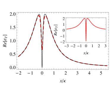
Figure 2: The real part of $\varepsilon_{T}$ vs. the normalized frequency detuning $x/\kappa$: $n=0$ (red-dashed) and $n=0.7$ (black-solid) with $\gamma_{m}=2\pi\times 14.1$ kHz and $\wp_{c}=1mW$. In the inset: $n=0.7$, $\gamma_{m}=2\pi\times 141$ Hz and $\wp_{c}=1mW$.

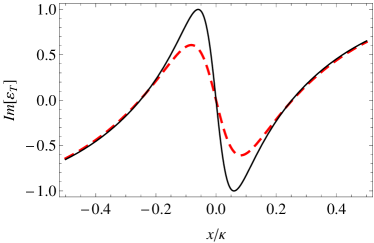
Figure 3: The imaginary part of $\varepsilon_{T}$ vs. the normalized frequency detuning $x/\kappa$: $n=0$ (red-dashed) and $n=0.7$ (black-solid) with $\gamma_{m}=2\pi\times 14.1$ kHz and $\wp_{c}=1mW$.

To see this clearly, in Fig. 2, we plot the $Re[\varepsilon_{T}]$ versus the normalized frequency $x/\kappa$ with $\gamma_{m}=2\pi\times 14.1$ kHz and $\wp_{c}=1mW$ for different $n$. We can see form Fig. 2 that when $n=0$ (i.e. the usual optomechanically induced transparency case), the optomechanically induced transparency dip will become shallow with a large mechanical decay $\gamma_{m}$ (red-dashed). However, when an additional blue-sideband driving field satisfying the condition $n=\sqrt{\gamma_{m}\kappa/2G^{2}}\approx 0.7$ applied, the transparency dip will become perfect, exhibiting totally transmission of probe laser (black-solid). Physically, it means that the dissipative energy through the decay $\gamma_{m}$ of the mechanical resonator can be compensated by applying the right-hand driving field with amplitude $\varepsilon_{d}=\varepsilon_{c}\sqrt{\gamma_{m}\kappa/2G^{2}}$ and the blue mechanical sideband frequency. When $\omega_{p}\approx\omega_{0}$, $n=\sqrt{\gamma_{m}\kappa/2G^{2}}$ and the beat frequency $\omega_{p}-\omega_{c}=\omega_{m}(x=0)$, thus, the MR is driven by a force oscillating at its eigenfrequency $\omega_{m}$ and the resonator starts to oscillate coherently. This motion will generate photons with frequency $\omega_{p}$ that interfere destructively with the probe beam, leading to a optomechanically induced transparency dip.

In Fig. 3, we plot the the dispersion curve $Im[\varepsilon_{T}]$ versus the normalized frequency $x/\kappa$ with $\gamma_{m}=2\pi\times 14.1$ kHz and $\wp_{c}=1mW$ for different $n$. Clearly, the curve with $n=0.7$ (black-solid) is much steeper than the one with $n=0$ (red-dashed) in the vicinity of $x=0$. It means that we can easily control the dispersive behavior of the optomechanical system by applying the blue-detuned driving field with amplitude $\varepsilon_{d}=n\varepsilon_{c}$, which can possibly be used to control slow light in optomechanical systems.

IV optomechanically induced amplification

In this section, we study the optomechanically induced amplification in this double-cavity optomechanical system. If the ratio $n>\sqrt{\gamma_{m}\kappa/2G^{2}}$, we find the $Re[\varepsilon_{T}]$ will become negative in the vicinity of $x=0$ (see the inset in Fig. 2). It means that optomechanically induced gain (amplification) can be realized in this double-cavity system by applying a blue-detuned driving field to the right-side cavity with amplitude $\varepsilon_{d}=n\varepsilon_{c}$. Note that when the system works under the condition $x=0$, $n=\sqrt{1+\frac{\gamma_{m}\kappa}{2G^{2}}}$, $Re[\varepsilon_{T}]$ will be divergent. In addition, the system will work into the parametric instability regime as $n\gtrsim 1$ when the input power $\wp_{c}=1$mW, and so we limit ourselves to the case where $n\leq 1$.

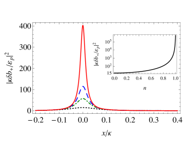
Figure 4: The normalized mechanical oscillation $|\kappa\delta b_{+}/\varepsilon_{p}|^{2}$ vs. the normalized frequency detuning $x/\kappa$: $n=0$ (black-dotted), $n=0.7$ (green-dotted-dashed), $n=0.8$ (blue-dashed), and $n=0.9$ (red-solid) with $\wp_{cL}=1mW$. In the inset, we plot the normalized mechanical oscillation $|\kappa\delta b_{+}/\varepsilon_{p}|^{2}$ vs. the ratio $n$.

In Fig. 4, we plot the mechanical oscillation $|\kappa\delta b_{+}/\varepsilon_{p}|^{2}$ (normalized to probe field $\varepsilon_{p}$) versus the normalized frequency $x/\kappa$ for different $n$. In the inset we plot the $|\kappa\delta b_{+}/\varepsilon_{p}|^{2}$ as a function of $n$ for $x=0$. It can be seen clearly from Fig. 4 that the mechanical oscillation peak value locates at $x=0$, and increases with $n$ [$n=0$ (black-dotted), $n=0.7$ (green-dotted-dashed), $n=0.8$ (blue-dashed), $n=0.9$ (red-solid)]. And when $n$ increases up to 1, the mechanical oscillation peak value will increase approximately to $6.1\times 10^{5}$ (see the inset in Fig. 4). It means that the optomechanical effect will become stronger for bigger $n$ (less than or equal to 1) when $\omega_{p}-\omega_{c}=\omega_{m}(x=0)$ and $\omega_{d}-\omega_{0}=\omega_{m}$. The reason for this is that, the blue-mechanical sideband (heating sideband) of right-hand cavity generating much phonons which will be absorbed by the Anti-Stokes processes in left-hand cavity for the red-mechanical sideband (cooling sideband). Then, the optomechanical effect of the double-cavity system is resonantly enhanced.

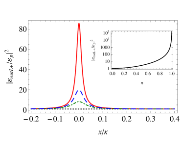
Figure 5: The normalized left-hand output energy $|\varepsilon_{outL+}/\varepsilon_{p}|^{2}$ vs. the normalized frequency detuning $x/\kappa$: $n=0$ (black-dotted), $n=0.7$ (green-dotted-dashed), $n=0.8$ (blue-dashed), and $n=0.9$ (red-solid) with $\wp_{cL}=1mW$. In the inset, we plot the normalized output energy $|\varepsilon_{outL+}/\varepsilon_{p}|^{2}$ vs. the ratio $n$.

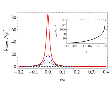
Figure 6: The normalized right-hand output energy $|\varepsilon_{outR-}/\varepsilon_{p}|^{2}$ vs. the normalized frequency detuning $x/\kappa$: the parameters are the same as in Fig. 4. In the inset, we plot the normalized output energy $|\varepsilon_{outR-}/\varepsilon_{p}|^{2}+1$ vs. the ratio $n$.

In Fig. 5-6, we plot the output power $|\varepsilon_{outL+}/\varepsilon_{p}|^{2}$ and $|\varepsilon_{outR-}/\varepsilon_{p}|^{2}$ normalized to the input probe field $\varepsilon_{p}$ respectively, versus the normalized frequency $x/\kappa$ for different $n$. It can be seen clearly from Fig. 5-6 that the output energies $|\varepsilon_{outL+}/\varepsilon_{p}|^{2}$ and $|\varepsilon_{outR-}/\varepsilon_{p}|^{2}$ get the maximum value at $x=0$ for a certain value $n$. When $x=0$, the output normalized energies $|\varepsilon_{outL+}/\varepsilon_{p}|^{2}$ and $|\varepsilon_{outR-}/\varepsilon_{p}|^{2}$ will increase with $n$ which is similar to the mechanical oscillation $|\kappa\delta b_{+}/\varepsilon_{p}|^{2}$. This is because that when $x=0$, the optomechanical effect will be strongest for a certain value $n$ as discussed above. The curves of the output normalized energies $|\varepsilon_{outL+}/\varepsilon_{p}|^{2}$ and $|\varepsilon_{outR-}/\varepsilon_{p}|^{2}$ almost have the same line shape, except that the output normalized energy $|\varepsilon_{outL+}/\varepsilon_{p}|^{2}$ starts from 1 with the increase of $n$ for $x=0$ while the output normalized energy $|\varepsilon_{outR-}/\varepsilon_{p}|^{2}$ starts from 0 (see the insets in Fig. 5-6). This shows that the double-cavity optomechanical system will be reduced to the standard one-cavity optomechanical model ($|\varepsilon_{outR-}/\varepsilon_{p}|^{2}=0$) when $n=0$. When $n$ increases up to 1, the output normalized energies $|\varepsilon_{outL+}/\varepsilon_{p}|^{2}$ and $|\varepsilon_{outR-}/\varepsilon_{p}|^{2}$ will increase approximately to $1.6\times 10^{5}$ (see the insets in Fig. 5-6). The reason for this is that, the existing of blue-detuned driving field with $\omega_{d}-\omega_{0}=\omega_{m}$ will coherently enhance the oscillation of the MR (see Fig. 4), leading to optomechanically induced amplification. Thus, we can realize the optomechanically induced amplification for a resonantly injected probe in the double-cavity optomechanical system by appropriately adjusting the ratio $n$ of the two strong field amplitudes $\varepsilon_{c,d}$.

V Conclusions

In summary, we have studied in theory a double-cavity optomechanical system driven by a red sideband laser from one side and a blue sideband one from the other side. Our analytical and numerical results show that if adjusting the amplitude-ratio of the two driving fields $n>\sqrt{\gamma_{m}\kappa/2G^{2}}$ , the optomechanically induced amplification for a resonantly incident probe (i.e., $\omega_{p}-\omega_{c}-\omega_{m}=0$) can be realized in this system. Typically, remarkable amplification can be obtained when $n\sim 1$. The reason for this is that, the Stokes processes in the blue-sideband driven cavity can generate phonons in the mechanical elements, and these phonons will be further absorbed by the Anti-Stokes processes in the red-sideband driven cavity. As a result, the optomechanical effect of the double-cavity system is resonantly enhanced. In addition, the perfect optomechanically induced transparency can be realized if we set the ratio $n=\sqrt{\gamma_{m}\kappa/2G^{2}}$. Different from usual optomechanical induced transparency, this phenomenon is robust to mechanical dissipation, namely, the perfect transparency window can preserve even if the mechanical resonator has a relatively large decay rate $\gamma_{m}$. We expect that our study can be used to realize signal quantum amplifier and light storage in the quantum information processes.

References

• (1) T. J. Kippenberg and K. J. Vahala, Science 321, 1172-1176 (2008).
• (2) F. Marquardt and S. M. Girvin, Physics 2, 40 (2009).
• (3) P. Verlot, A. Tavernarakis, T. Briant, P.-F. Cohadon, and A. Heidmann, Phys. Rev. Lett. 104, 133602 (2010).
• (4) S. Mahajan, T. Kumar, A. B. Bhattacherjee, and ManMohan, Phys. Rev. A 87, 013621 (2013).
• (5) S. Gigan, H. B$\ddot{o}$hm, M. Paternostro, F. Blaser, G. Langer, J. Hertzberg, K. Schwab, D. B$\ddot{a}$uerle, M. Aspelmeyer, and A. Zeilinger, Nature (London) 444, 67-70 (2006).
• (6) D. Kleckner and D. Bouwmeester, Nature (London) 444, 75-78 (2006).
• (7) G. S. Agarwal and Sumei Huang, Phys. Rev. A 81, 041803(R) (2010).
• (8) T. J. Kippenberg and K. J. Vahala, Opt. Express 15, 17172-17205 (2007).
• (9) D. K. Armani, T. J. Kippenberg, S. M. Spillane, and K. J. Vahala, Nature (London) 421, 925-928 (2003).
• (10) A. Schliesser, R. Rivi$\grave{e}$re, G. Anetsberger, O. Arcizet, and T. J. Kippenberg, Nat. Phys. 4, 415-419 (2008).
• (11) M. Eichenfield, J. Chan, R. M. Camacho, K. J. Vahala and O. Painter, Nature 462, 78 (2009).
• (12) Y. Li, J. Zheng, J. Gao, J. Shu, M. S. Aras and C. W. Wong, Opt. Express 18, 23844 (2010)
• (13) J. D. Thompson, B. M. Zwickl, A. M. Jayich, F. Marquardt, S. M. Girvin and J. G. E. Harris, Nature 452, 72 (2008).
• (14) Cheung H K and Law C K, Phys. Rev. A 84, 023812 (2011).
• (15) F. Brennecke, S. Ritter, T. Donner and T. Esslinger, Science 322, 235 (2008).
• (16) K. Zhang, P. Meystre and W. Zhang, Phys. Rev. Lett. 108, 240405 (2012).
• (17) C. A. Regal, J. D. Teufel and K. W. Lehnert, Nat. Phys. 4, 555 (2008).
• (18) Z. L. Xiang, S. Ashhab, J. Q. You and F. Nori, Rev. Mod. Phys. 85, 623 (2013).
• (19) I. Wilson-Rae, N. Nooshi, W. Zwerger and T. J. Kippenberg, Phys. Rev. Lett. 99, 093901 (2007).
• (20) F. Marquardt, J. P. Chen, A. A. Clerk, and S. M. Girvin, Phys. Rev. Lett. 99, 093902 (2007).
• (21) Y. Li, L. A. Wu, and Z. D. Wang, Phys. Rev. A 83, 043804 (2011).
• (22) J. M. Dobrindt, I. Wilson-Rae, and T. J. Kippenberg, Phys. Rev. Lett. 101, 263602 (2008).
• (23) S. Gr$\ddot{o}$blacher, K. Hammerer, M. Vanner, and M. Aspelmeyer, Nature (London) 460, 724-727 (2009).
• (24) S. Weis, R. Rivi$\grave{e}$re, S. Del$\acute{e}$glise, E. Gavartin, O. Arcizet, A. Schliesser, and T. J. Kippenberg, Science 330, 1520-1523 (2010).
• (25) G. S. Agarwal and Sumei Huang, Phys. Rev. A 81, 041803(R) (2010).
• (26) A. Kronwald and F. Marquardt, Phys. Rev. Lett. 111, 133601 (2013).
• (27) D. E. Chang, A. H. Safavi-Naeini, M. Hafezi, and O. Painter, New J. Phys. 13, 023003 (2011).
• (28) V. Fiore, Y. Yang, M. C. Kuzyk, R. Barbour, L. Tian, and H. Wang, Phys. Rev. Lett. 107, 133601 (2011).
• (29) T. Kippenberg, H. Rokhsari, T. Carmon, A. Scherer, and K. Vahala, Phys. Rev. Lett. 95, 033901 (2005).
• (30) F. Marquardt, J. G. E. Harris, and S. M. Girvin, Phys. Rev. Lett. 96, 103901 (2006).
• (31) K. Vahala, M. Herrmann, S. Kn$\ddot{u}$nz, V. Batteiger, G. Saathoff, T. W. H$\ddot{a}$nsch, and T. Udem, Nat. Phys. 5, 682 (2009).
• (32) F. Massel, T. T. Heikkil$\ddot{a}$, J. M. Pirkkalainen, S. U. Cho, H. Saloniemi, P. J. Hakonen, and M. A. Sillanp$\ddot{a}\ddot{a}$, Nature, 480, 351 (2011).
• (33) A. H. Safavi-Naeini, T. P. Mayer Alegre, J. Chan, M. Eichenfield, M. Winger, Q. Lin, J. T. Hill, D. E. Chang, and O. Painter, Nature, 472, 69 (2011).
• (34) A. Nunnenkamp, V. Sudhir, A. K. Feofanov, A. Roulet, and T. J. Kippenberg, arXiv: 1312.5867 (2013).
• (35) A. Metelmann and A. A. Clerk, Phys. Rev. Lett. 112, 133904 (2014).
• (36) X. B. Yan, C. L. Cui, K. H. Gu, X. D. Tian, C. B. Fu, and J. H. Wu, Opt. Express, 22, 4886 (2014).
• (37) D. F. Walls and G. J. Milburn, “Quantum Optics” (Springer-Verlag, Berlin, 1994).