PostScript file created: ;  time 1341 minutes

LIKELIHOOD ANALYSIS OF EARTHQUAKE FOCAL MECHANISM DISTRIBUTIONS

Yan Y. Kagan and David D. Jackson

Department of Earth and Space Sciences, University of California,

Los Angeles, California 90095-1567, USA;

Emails: kagan@moho.ess.ucla.edu, david.d.jackson@ucla.edu

Short running title: Likelihood Analysis of Focal Mechanisms

Corresponding author contact details:

Office address: Dr. Y. Y. Kagan, Department Earth and Space Sciences (ESS), Geology Bldg, 595 Charles E. Young Dr., University of California Los Angeles (UCLA), Los Angeles, CA 90095-1567, USA

Office phone 310-206-5611

FAX: 310-825-2779

E-mail: kagan@moho.ess.ucla.edu

SECTION: SEISMOLOGY

SUMMARY In our paper published earlier we discussed forecasts of earthquake focal mechanism and ways to test the forecast efficiency. Several verification methods were proposed, but they were based on ad-hoc, empirical assumptions, thus their performance is questionable. In this work we apply a conventional, likelihood method to measure a skill of forecast. The advantage of such an approach is that earthquake rate prediction can in principle be adequately combined with focal mechanism forecast, if both are based on the likelihood scores, resulting in a general forecast optimization. To calculate the likelihood score we need to compare actual forecasts or occurrences of predicted events with the null hypothesis that the mechanism’s 3-D orientation is random. For double-couple source orientation the random probability distribution function is not uniform, which complicates the calculation of the likelihood value. To better understand the resulting complexities we calculate the information (likelihood) score for two rotational distributions (Cauchy and von Mises-Fisher), which are used to approximate earthquake source orientation pattern. We then calculate the likelihood score for earthquake source forecasts and for their validation by future seismicity data. Several issues need to be explored when analyzing observational results: their dependence on forecast and data resolution, internal dependence of scores on forecasted angle, and random variability of likelihood scores. In this work we propose a preliminary solution to these complex problems, as these issues need to be explored by a more extensive statistical analysis.

Key words: Probabilistic forecasting; Earthquake interaction, forecasting, and prediction; Seismicity and tectonics; Theoretical seismology; Statistical seismology; Dynamics: seismotectonics.

1 Introduction

Kagan & Jackson (2014) discussed two problems: forecasting earthquake focal mechanisms and evaluating a forecast skill. The first problem was initially addressed by Kagan & Jackson (1994), but no attempt verifying the forecast has been carried out until now. Kagan & Jackson (2014) proposed several verification methods, but the techniques were based on ad-hoc, empirical assumptions, thus their performance is not clear. In this work we apply a conventional, likelihood method to measure the skill of a forecast.

The likelihood estimate for the focal mechanism prediction compares actual forecasts or later occurrences of predicted events with the null hypothesis that the mechanism’s orientation is random. It is similar to our forecast testing for long- or short-term earthquake rate predictions (Kagan & Jackson, 1994, 2011), where we use a uniform Poisson process in space or time as the null hypothesis. With the earthquake source orientation distribution, the situation is more complex, the probability distribution function (PDF) is not uniform, though its analytical expression is known: see Kagan (1990, eq. 3.1) or Table 3 for orthorhombic symmetry by Grimmer (1979).

Kagan & Jackson (1994, 2011) approximate earthquake rate forecast by smoothing the past seismicity record with a spatial kernel. They optimize the kernel by searching for the best prediction of future seismicity level (see also Molchan, 2012). The assumption is that the true model belongs to a general class of parametric models which is used to approximate seismicity. Right now we adjust only a width of the smoothing kernel and its functional form. In principle though several other kernel parameters (such as its directivity, magnitude dependence, etc.) can be optimized (see, for instance, Kagan & Jackson, 2011).

To measure the forecast skill several likelihood scores are calculated (Kagan, 2009, Table 3), most of these scores ($I_{0}$, $I_{1}$, $I_{2}$, and $I_{3}$) have similar values, their difference is due to forecast map resolution and other known and controlled factors. This feature is explained by our smoothing forecast procedure which yields a relatively smooth seismicity map.

A major problem with the focal mechanism forecast is that we lack a model for earthquake source pattern similar to that for earthquake rate. Thus our forecast distribution contains many relatively sharp steps, and if integrated they produce the $I_{4}$ score (Kagan, 2009, Table 3), which yields a consistent estimate that converges to the true value only when the sample size tends to infinity (Kagan, 2007; Molchan, 2010). Therefore in this work we are trying to find the properties of $I_{4}$ score for the earthquake catalogs under investigation. Nevertheless, we hope that this new measure of focal mechanism forecast skill would be useful in earthquake prediction efforts.

2 Statistical focal mechanism forecasts

Kagan & Jackson (2014) analyzed the focal mechanism orientation distribution in the Global Centroid-Moment-Tensor (GCMT) catalog (Ekström et al. 2012, and its references, see Fig. 1 in Kagan & Jackson, 2014). Kagan & Jackson (2014) considered $\Phi_{1}$ angle which is the average rotation angle between the forecasted weighted focal mechanisms and the mechanisms of the 1977-2007 earthquakes in a 1000 km circle surrounding this predicted event. The $\Phi_{2}$ angle is the angle between the forecasted mechanism and the double-couple ($DC$) mechanism of the observed events in the 2008-2012 period.

In this work we limited our study to the forecast in the latitude bandwidth $[75^{\circ}S-75^{\circ}N]$, because calculations in this range take considerably less time. Moreover, almost all earthquakes in the GCMT catalog are concentrated there (Kagan & Jackson, 2014, Fig. 2).

In Fig. 1 we display a scatterplot of two angles $\Phi_{1}$ and $\Phi_{2}$. To investigate the interdependence of two angles, we subdivide the plot of 1069 $\Phi_{1}$ angles into ten subsets with an increasing angle and calculate the quantiles of $\Phi_{2}$ distribution in each of these subsets.

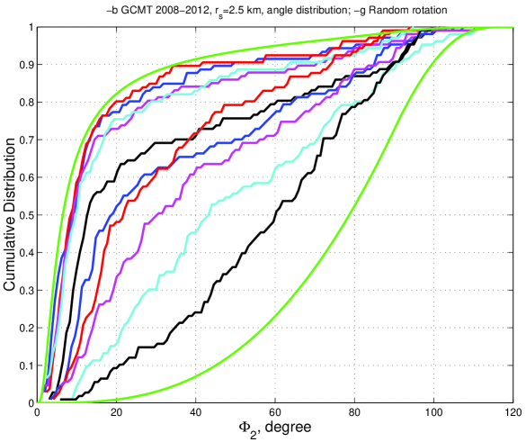
Figure 4: GCMT catalog, 2008–2012, $r_{s}=2.5$ km, latitude range $[75^{\circ}S-75^{\circ}N]$,

The focal mechanism forecast is displayed in Fig. 4 of Kagan & Jackson (2014). About 42% of the cells in the forecast have variables $\Phi_{1}$ and $\Phi_{2}$ equal to zero. These cell centers do not have any earthquake centroid within 1000 km distance. To avoid future ‘surprises’, in our earthquake rate forecasts we assume that 1% of all earthquakes occur uniformly over the Globe (Jackson & Kagan 1999; Kagan & Jackson 2011). We did not make such or similar an assumption for the focal mechanism forecast, since it is not known what default value needs to be adopted for these cells (Kagan & Jackson, 2014).

However, almost all 2008-2012 earthquakes occurred in the places within 1000 km of 1977-2007 epicentroids, thus their angles could be evaluated. Only 3 events out of 1069 are outside of the 1000 km limit. In Fig. 1 these zero values of $\Phi_{1}$ and $\Phi_{2}$ are all plotted at the point [0.0, 0.0] and thus are not separately visible. In our likelihood studies below we sometimes use only 1066 events for which the angles can be measured.

In Table 1 we list the properties of both angles distribution shown in Fig. 1. The average $\Phi_{2}$ value increases steadily with the increase of $\Phi_{1}$, though the standard deviation is generally stable, thus the coefficient of variation also decreases for later subsets. In Fig. 7 by Kagan & Jackson (2014) this interdependence of two angles was characterized by regression lines.

3 Rotation angle distributions

Kagan (2013, Section 5) considers three statistical distributions for the double-couple ($DC$) source orientation: $\bullet$ 1. The uniform random rotation, which corresponds to orthorhombic symmetry for a general $DC$ source. This distribution is defined for the orientation angle range $0^{\circ}-120^{\circ}$. The probability density function (PDF) is

$$f(\Phi)\ =\ (4/\pi)(1-\cos\Phi)\quad{\rm for}\quad 0\leq\Phi\leq 90^{\circ}\,;$$ (1)

$$f(\Phi)\ =\ (4/\pi)(3\sin\Phi+2\cos\Phi-2)\quad{\rm for}\quad 90^{\circ}\leq\Phi\leq\Phi_{S}\,;$$ (2)

and

$$f(\Phi)\ =\ (4/\pi)\,\Bigg{\{}3\sin\Phi+2\cos\Phi-2\,-$$ (3)

$$(6/\pi)\bigg{[}2\,\sin\Phi\,\arccos\left({{1+\cos\Phi}\over{-2\cos\Phi}}\right)^{1/2}-$$

$$(1-\cos\Phi)\,\arccos{{1+\cos\Phi}\over{-2\cos\Phi}}\,\bigg{]}\Bigg{\}}\quad{\rm for}\quad\Phi_{S}\leq\Phi\leq 120.0^{\circ}\,,$$

where

$$\Phi_{S}\ =\ 2\arccos\,(3^{-1/2})\ =\ \arccos\,\left(-\,{1\over 3}\right)\ \approx\ 109.47^{\circ}\,.$$ (4)

$\bullet$ 2. Two non-uniform statistical distributions: the rotational Cauchy law (Kagan 1992) and the rotational von Mises-Fisher (VMF) law (Kagan 2000; Mardia & Jupp 2000, pp. 289-292; Morawiec 2004, pp. 88-89).

The Cauchy law in the 3-D Euclidean space is scale-invariant for relatively small angles and it has a power-law tail for large angles. The rotational Cauchy is defined on the 3-D hypersphere of a normalized quaternion (Kagan 1982; 1990). The PDF of the rotational Cauchy distribution can be written as

$$f(\Phi)\ =\ {{2}\over{\pi}}\Biggr{[}{{\kappa A^{2}(1+A^{2})}\over{(\kappa^{2}+A^{2})^{2}}}\Biggl{]}\ =\ {{4\,\kappa\,\left[1-\cos({\Phi})\right]}\over{\pi\,{{\left[1+{\kappa^{2}}+\left({\kappa^{2}}-1\right)\,\cos({\Phi})\right]}^{2}}}}\,,\quad{\rm for}\quad 0^{\circ}\leq\Phi\leq 180^{\circ}\,,$$ (5)

where $A=\tan(\Phi/2)$.

Similarly to the rotational Cauchy law the von Mises-Fisher distribution is a Gaussian-shaped function defined on the 3-D hypersphere of a normalized quaternion. It is concentrated near the zero angle $\Phi)$. This distribution can be implemented to model random errors in determining focal mechanisms.

Fig. 2 displays the $DC$ random rotation distribution (Eqs. 1–4), as well as several Cauchy distributions. The Cauchy distribution (5) has only one parameter ($\kappa$), a smaller $\kappa$-value corresponds to the rotation angle $\Phi_{\rm min}$ concentrated closer to zero. These theoretical laws can be compared to the cumulative $\Phi_{1}$ and $\Phi_{2}$ angle distributions. The Cauchy law approximates the $\Phi_{1}$ curve reasonably well for $\kappa=0.075$ up to about 20^∘. Even for larger angles the observation curve is close to the Cauchy law lines. A similar effect is observed for the $\Phi_{2}$ curve.

The VMF distribution is obtained by generating a 3-D normally distributed random variable u ($u_{1}$, $u_{2}$, $u_{3}$) with the standard deviation $\sigma_{\bf u}$ ($\sigma_{u_{1}},\,\sigma_{u_{2}},\,\sigma_{u_{3}}$) and then calculating the unit quaternion

$$q_{0}\ =\ 1/\sqrt{1+u_{1}^{2}+u_{2}^{2}+u_{3}^{2}}\,,$$

$$q_{i}\ =\ u_{i}/\sqrt{1+u_{1}^{2}+u_{2}^{2}+u_{3}^{2}}\,,\quad{\rm for}\ i=1,2,3.$$ (6)

The 3-D rotation angle is calculated

$$\Phi\ =\ 2\arccos(q_{0})\,.$$ (7)

Since components of the vector u are normally distributed, the sum ($u_{1}^{2}+u_{2}^{2}+u_{3}^{2}$) in Eq. 6 follows the Maxwell distribution. The Maxwell equation describes the distribution of a vector length in three dimensions, if the vector components have a Gaussian distribution with a zero mean and a standard error $\sigma_{u}$. For small $\sigma_{u}$ the distribution of angle $\Phi$ follows the Maxwell law (Kagan, 2013).

These Cauchy and VMF laws are theoretically defined for orientation angle range $0^{\circ}-180^{\circ}$. However, because of the orthorombic symmetry of the general $DC$ source (Kagan, 2013) its maximum disorientation cannot exceed $120^{\circ}$. Since we cannot obtain an analytical representation for these distributions, we use simulation (Kagan, 1992) to derive the distribution form for the range $0^{\circ}-120^{\circ}$.

In Fig. 3 the focal mechanism angles are compared to the VMF distribution. As expected (see Kagan, 2013) the fit of the VMF law to observation curve is not as good as for the Cauchy distribution, which provides a much better approximation (Fig. 2).

4 Error diagrams

Table 2 shows the values of the information scores, $I$, (Kagan, 2009) for two theoretical distributions. As can be seen from Figs. 2 and 3 the curves that are close to the random rotation line have the score value closer to zero.

There are considerable problems in computing the information score for the rotation angles $\Phi_{1}$ and $\Phi_{2}$ in the GCMT catalog. As Kagan (2009) discusses, we have a reasonable model for the earthquake rate forecast: future earthquakes are concentrated close to the location of the past events, thus our general forecast model is obtained by smoothing the past earthquake locations to infer the spatial distribution for future events. We evaluate the smoothing kernel parameters using some optimal criteria (Kagan & Jackson, 2011). The error or concentration diagrams for the forecast maps are relatively smooth so that various methods for evaluating the scores ($I_{0}$, $I_{1}$, $I_{2}$, and $I_{3}$) yield similar results Kagan (2009, Table 3).

However, no such general model is yet available for the distributions of angles $\Phi_{1}$ and $\Phi_{2}$. Since the number of observations is relatively small, the concentration diagrams or cumulative distributions for these angles contains step-like jumps. Thus, we can calculate the score which Kagan (2009) called $I_{4}$, the estimate of which is biased for small samples (Kagan, 2007).

$$I_{4}\,=\,{1\over n}\sum_{i=1}^{n}\nu_{i}\,\log_{2}\left[{{\nu_{i}}/\sum_{k_{i-1}}^{k_{i}}{\tau_{i}}}\right]\,,$$ (8)

where $\tau$ is the cumulative fraction of the alarm time, $\nu$ is the cumulative fraction of failures to predict, and $k_{i}$ is the cell number corresponding to the $i$-th event, $\log_{2}$ is used to obtain the score measured in the Shannon bits of information (Kagan, 2009).

In Table 3 several estimates of the $I_{4}$ score are shown for both angles and for two choices of smoothing kernel width ($r_{s}$). We subdivide the angle range ($0^{\circ}-120^{\circ}$) into various grid cells to see how it influences the $I_{4}$-value. The number of cells with non-zero number of events is relatively small for large cell size, but for a finer subdivision it approaches the total number of angle measurements (1066). The score value also approaches an upper limit for a finer subdivision. The results do not appear to depend on the $r_{s}$-value.

The final $I_{4}$-values can be reasonably well forecasted by comparing their approximation by the Cauchy distribution in Fig. 2 with the appropriate score values in Table 2. For example, the major part of the $\Phi_{1}$ curve is between Cauchy curves $\kappa=0.05$ and $\kappa=0.075$, and the score value is also between the respective values in Table 2.

Table 4 shows the values of the information scores for the 2008-2012 GCMT catalog in a format similar to Table 3 by Kagan (2009). We vary several parameters to investigate the dependence of scores. For example, the scores change with the grid modification, partly because almost all the events are located in separate cells for a higher-resolution forecast. However, since the score $I_{2}$ is calculated for the actual earthquake location in the test period, their value does not depend on the cell size, as expected.

The influence of the smoothing kernel width ($r_{s}$) on the score looks insignificant. More study is necessary to optimize our forecast by changing ($r_{s}$); unfortunately the needed computations are very extensive.

Fig. 4 displays cumulative $\Phi_{2}$ distributions for 10 subsets shown in Fig. 1 and Table 1. The distributions move from left to right; the distribution for the first subset is close to the Cauchy $\kappa=0.025$ law curve, whereas the last distribution is close to the random curve. The score values shown in the last column of Table 1 confirm this pattern: for the initial subsets $I_{4}$-value is close to that $\kappa=0.25$ Cauchy distribution (see Table 2), whereas for the 10-th subset $I_{4}$-value approaches zero.

5 Discussion

The advantage of the likelihood approach for focal mechanism orientation is that the likelihood scores for earthquake rate prediction can be adequately combined with the focal mechanism forecast, resulting in a general earthquake forecast optimization.

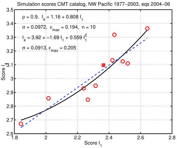
Figure 5: GCMT catalog, 2004–2006, NW Pacific, $r_{s}=15$ km,

As we observed (Kagan, 2009) the $I_{4}$ score estimates are biased and have a higher random variation compared to the other information scores. In order to understand the properties of the $I_{4}$ score we study a correlation between $I_{4}$ and other scores. To investigate the relation between the two scores, $I_{1}$ and $I_{4}$, in Fig. 5 we calculated these scores for 10 simulated catalogs shown in Fig. 10 (Kagan, 2009). The range of $I_{1}$ values (0.8) can be compared with the standard deviation for $I_{0}$ ($\sigma_{n}=0.215$), shown in Table 3 by Kagan (2009). The scores $I_{0}$ and $I_{1}$ are optimized to have close values. As the diagram demonstrates, $I_{4}$ is usually larger than $I_{1}$, but their correlation coefficient is high, thus one can estimate the $I_{1}$ score using regression.

As mentioned in the Introduction, a significant effort needs to be extended to incorporate the methods developed in this and the previous (Kagan & Jackson, 2014) publications to forecast earthquake focal mechanisms. A similar investigation needs to be carried out to fully optimize the global earthquake rate forecast (Kagan & Jackson, 2011). However, these efforts will be mostly of technical nature, the major forecast scientific issues are addressed in this and above-mentioned papers.

6 Conclusions

$\bullet$  1. We apply a likelihood method to measure the skill of an earthquake focal mechanism forecast. The advantage of such an approach is that the likelihood scores for the earthquake rate prediction can quantitatively be combined with the focal mechanism forecast, resulting in a general forecast optimization. $\bullet$  2. We compare actual forecasts or occurrences of event source properties with the null hypothesis that the mechanism’s 3-D orientation is random. $\bullet$  3. We calculate the information (likelihood) score for two rotational distributions (Cauchy and von Mises-Fisher) which are used to approximate a source orientation pattern. $\bullet$  4. We calculate the likelihood score for earthquake source forecasts based on the GCMT catalog and their validation by future seismicity data. We explored the dependence of the results on data resolution, internal dependence of scores on forecasted angle, and a random variability of likelihood scores.

Acknowledgments

The authors appreciate support from the National Science Foundation through grants EAR-0711515, EAR-0944218, and EAR-1045876, as well as from the Southern California Earthquake Center (SCEC). SCEC is funded by NSF Cooperative Agreement EAR-0529922 and USGS Cooperative Agreement 07HQAG0008. Publication 0000, SCEC.

References

Ekström, G., M. Nettles & A.M. Dziewonski, 2012. The global CMT project 2004-2010: Centroid-moment tensors for 13,017 earthquakes, Phys. Earth Planet. Inter., 200-201, 1-9.

Grimmer, H., 1979. Distribution of disorientation angles if all relative orientations of neighboring grains are equally probable, Scripta Metallurgica, 13(2), 161-164, DOI: 10.1016/0036-9748(79)90058-9.

Jackson, D. D. & Y. Y. Kagan, 1999. Testable earthquake forecasts for 1999, Seism. Res. Lett., 70(4), 393-403.

Kagan, Y. Y., 1991. 3-D rotation of double-couple earthquake sources, Geophys. J. Int., 106(3), 709-716.

Kagan, Y. Y., 1992. Correlations of earthquake focal mechanisms, Geophys. J. Int., 110(2), 305-320.

Kagan, Y. Y., 2000. Temporal correlations of earthquake focal mechanisms, Geophys. J. Int., 143(3), 881-897.

Kagan, Y. Y., 2007. On earthquake predictability measurement: information score and error diagram, Pure Appl. Geoph., 164(10), 1947-1962.

Kagan, Y. Y., 2009. Testing long-term earthquake forecasts: likelihood methods and error diagrams, Geophys. J. Int., 177(2), 532-542.

Kagan, Y. Y., 2013. Double-couple earthquake source: symmetry and rotation, Geophys. J. Int., 194(2), 1167-1179, doi: 10.1093/gji/ggt156

Kagan, Y. Y. & D. D. Jackson, 1994. Long-term probabilistic forecasting of earthquakes, J. Geophys. Res., 99, 13,685-13,700.

Kagan, Y. Y. & D. D. Jackson, 2011. Global earthquake forecasts, Geophys. J. Int., 184(2), 759-776.

Kagan, Y. Y. & D. D. Jackson, 2014. Statistical earthquake focal mechanism forecasts, Geophys. J. Int., 197(1), 620-629.

Mardia, K. V. & P. E. Jupp 2000. Directional Statistics, Chichester, New York, Wiley, 429 pp.

Molchan, G., 2010. Space-time earthquake prediction: the error diagrams, Pure Appl. Geoph., (The Frank Evison Volume), 167(8/9), 907-917. doi: 10.1007/s00024-010-0087-z.

Molchan, G., 2012. On the Testing of Seismicity Models, Acta Geophysica, 60(3), 624-637, doi: 10.2478/s11600-011-0042-0.

Morawiec, A. 2004. Orientations and Rotations: Computations in Crystallographic Textures, Springer/Berlin, New York, pp. 200.

No.	$\Phi_{1}$	$<\Phi_{2}>$	$\sigma_{\Phi}$	$C_{v}$	n	$I_{4}$
	∘	∘	∘	Coef.		Score
1	2	3	4	5	6	7
1	0.2	18.0	23.3	1.29	106	6.56
2	6.4	17.3	21.6	1.25	106	6.47
3	9.5	20.8	25.6	1.23	107	5.93
4	12.1	20.7	24.6	1.19	106	5.85
5	15.1	30.6	30.9	1.01	107	4.32
6	18.8	34.5	29.7	0.86	107	3.35
7	23.5	31.7	24.0	0.76	106	3.42
8	29.4	40.4	28.3	0.70	107	2.36
9	36.4	50.4	28.9	0.57	106	1.45
10	47.2	58.4	24.4	0.42	108	0.77

Table 1: Values of observed rotation angle $\Phi_{2}$ for 10 subsets of scatterplot of two angles $\Phi_{1}$ and $\Phi_{2}$ (see Fig. 1). The beginning value of the $\Phi_{1}$ interval is shown in column 2. $<\Phi_{2}>$ is the average angle, $\sigma_{\Phi}$ is the standard deviation, $C_{v}$ is the coefficient of variation ($C_{v}={\sigma_{\Phi}\over<\Phi>}$) for angle $\Phi_{2}$, $n$ the number of events in a subset, and $I_{4}$ is the information score in bits.

#	Parameter	Score	Parameter	Score
	Cauchy ($\kappa$)		VMF ($\sigma_{u}$)
1	0.025	7.48	0.050	8.15
2	0.050	4.86	0.100	5.21
3	0.075	3.49	0.200	2.44
4	0.100	2.60	0.300	1.03
5	0.200	0.95	0.400	0.30
6	0.500	0.05	0.500	0.03

Table 2: Information scores in bits for theoretical distributions (see Section 3). $\kappa$ is the parameter of the rotational Cauchy distribution (see Fig. 2), $\sigma_{u}$ ditto for the von Mises-Fisher (VMF) rotational distribution (see Fig. 3).

#	Subdivision	$\xi$	$\Phi_{1}$	$\xi$	$\Phi_{2}$	$\xi$	$\Phi_{1}$	$\xi$	$\Phi_{2}$
		$r_{s}=2.5$ km				$r_{s}=6.0$ km
1	120	70	4.18	108	3.49	69	4.04	108	3.48
2	1200	448	4.41	538	3.74	452	4.28	531	3.70
3	12000	955	4.74	975	4.03	957	4.59	952	4.03
4	120000	1058	4.94	1053	4.18	1049	4.76	1057	4.23
5	1200000	1064	4.97	1065	4.24	1050	4.77	1057	4.23

Table 3: Information scores in bits for $\Phi_{1}$ and $\Phi_{2}$ angles (see Section 1) in the GCMT catalog, $r_{s}$ is the width of the smoothing kernel, $\xi$ is the total number of non-zero intervals (out of 1066 possible).

#		2008-2012, $[75^{\circ}S-75^{\circ}N]$
	Grid	$0.1^{\circ}$	$0.5^{\circ}$	$0.5^{\circ}$
	$r_{s}$	2.5 km	2.5 km	6.0 km
	$\xi$	1025	758	758
	Score
1	$I_{0}$	4.30	4.25	3.73
2	$I_{1}$	4.01	3.84	3.96
3	$I_{2}$	3.98	3.98	4.07
4	$I_{3}$	4.29	4.25	3.73
5	$I_{4}$	4.99	4.85	4.86

Table 4: Information scores in bits for one event, $r_{s}$ is the width of the smoothing kernel, $\xi$ is the total number of non-zero intervals (out of 1069 possible).

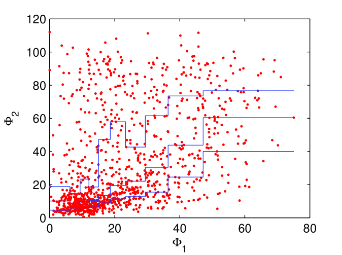
Figure 1: Distribution of rotation angles

in the Global Centroid Moment Tensor (GCMT) catalog, 1977–2007/2008–2012, latitude range $[75^{\circ}S-75^{\circ}N]$, earthquake number $n=1069$. Scatterplot of interdependence of the predicted $\Phi_{1}$ and observed $\Phi_{2}$ angles. Blue lines from top to bottom are 75%, 50%, and 25% quantiles, for a $\Phi_{1}$ angle subdivision with equal number of events in 10 subsets.

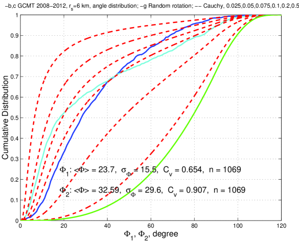
Figure 2: GCMT catalog, 1977–2007, $r_{s}=6$ km, latitude range $[75^{\circ}S-75^{\circ}N]$,

earthquake number $n=1069$. Blue and cyan curves are cumulative distributions of predicted rotation angle $\Phi_{1}$ and of observed rotation angle $\Phi_{2}$ at earthquake centroids, respectively. The dashed lines from left to right are for the Cauchy rotational distribution with $\kappa=0.025,0.050,0.075,0.1,0.2,0.5$. Right green solid line is for the random rotation. Distribution analysis results for angles $\Phi_{1}$ and $\Phi_{2}$ are written at the bottom of the plot: $<\Phi>$ is average rotation angle, $\sigma_{\Phi}$ its standard deviation, $C_{v}={\sigma_{\Phi}\over<\Phi>}$ its coefficient of variation.

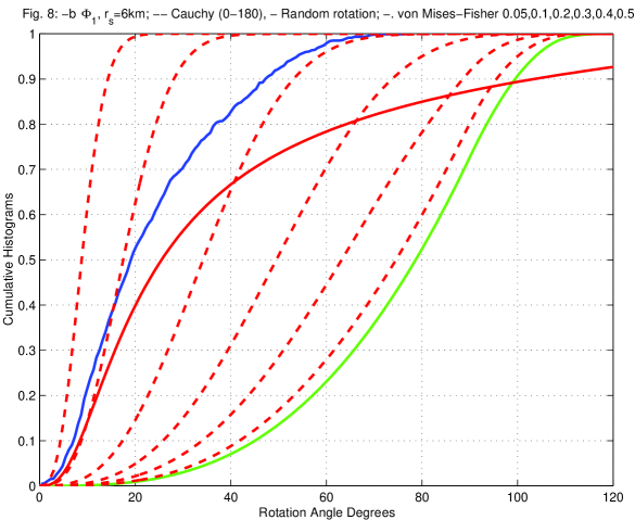
Figure 3: GCMT catalog, $r_{s}=6$ km, latitude range $[75^{\circ}S-75^{\circ}N]$,

1977–2007/2008–2012, earthquake number $n=1069$. Blue curve is the cumulative distribution of predicted rotation angle $\Phi_{1}$ at earthquake centroids. The dashed lines from left to right are for the von Mises-Fisher (VMF) rotational distribution with $\sigma_{u}=0.05,0.1,0.2,0.3,0.4,0.5$. Right green solid line is for the random rotation. Red solid curve is for the rotational Cauchy distribution with the domain $[\,0^{\circ}$ – $180^{\circ}]$.

earthquake number $n=1066$. Curves are cumulative distributions of the observed rotation angle $\Phi_{2}$ at earthquake centroids, for 10 subsets (see Fig. 1 and Table 1). Right green solid line is for the random rotation, left green solid curve is for the rotational Cauchy distribution with $\kappa=0.025$.

earthquake number $n=108$. Relation between two scores $I_{1}$ and $I_{4}$ in bits, shown by circles, for first 10 simulated catalogs, displayed in Fig. 10 by Kagan (2009). We calculate two regression lines approximating the interdependence of the $I_{1}$ and $I_{4}$ scores, the linear and quadratic curves. The coefficient of correlation $\rho$ between the angles is high $0.9$, indicating that the $I_{4}$ estimate can be well evaluated by $I_{1}$ regression. Results of both regressions are written at the top of the plot: $\sigma$ – standard error, $\varepsilon_{max}$ – maximum difference. A cross sign inside a square shows $I_{1}$ and $I_{4}$ estimates for the NW Pacific region from Table 3 by Kagan (2009).