Discoveries far from the Lamppost with Matrix Elements and Ranking

Abstract

The prevalence of null results in searches for new physics at the LHC motivates the effort to make these searches as model-independent as possible. We describe procedures for adapting the Matrix Element Method for situations where the signal hypothesis is not known a priori. We also present general and intuitive approaches for performing analyses and presenting results, which involve the flattening of background distributions using likelihood information. The first flattening method involves ranking events by background matrix element, the second involves quantile binning with respect to likelihood (and other) variables, and the third method involves reweighting histograms by the inverse of the background distribution.

Introduction.   The CERN Large Hadron Collider (LHC) will soon resume operation, probing energies never before accessed with colliders. Ideas about what sort of new physics it will discover often focus on models that resolve the hierarchy problem hierarchy or provide relic dark matter candidates DM . There are a great variety of ideas in each category. However, the lack of convincing evidence for new physics at the LHC to date suggests that we may be looking in the wrong places. We therefore consider methods that will allow the discovery of any departure from known physics.

The Matrix Element Method (MEM) MEM and similar multivariate analyses MVA have been used with success in LHC experiments. A particularly dramatic example has been the use of the MEM in the four-lepton channel for the discovery of the Higgs Boson Higgs Discovery and the measurement of its properties Higgs Properties . Such analyses used variables, such as MELA KD MELA or MEKD MEKD that involve the ratio of signal and background matrix elements. Clearly these variables are, therefore, optimized to the appropriate signal and background hypotheses.

A natural question is whether we can preserve, to some degree, the sensitivity of the MEM without assuming a specific signal hypothesis. We argue that this is possible. Specifically, one can use the log likelihood of events, calculated using the likelihood for background events, as a test statistic in a way that allows a model-independent discovery of new physics. We then demonstrate how the optimal MEM-based (as well as other) techniques can be used to create flat distributions for the background with respect to kinematic variables of interest, including, most importantly, variables derived from the matrix element.

The Matrix Element Method.   According to the Neyman-Pearson lemma NP , the optimal test statistic for comparing hypotheses $H_{0}$ and $H_{1}$ is provided by the likelihood ratio:

$$R_{\Lambda}(H_{0},H_{1})=\frac{\Lambda_{H_{0}}(\{{\mathcal{E}}_{i}\})}{\Lambda_{H_{1}}(\{{\mathcal{E}}_{i}\})},$$ (1)

where $\Lambda_{H_{0}}(\Lambda_{H_{1})}$ is the likelihood for the hypothesis $H_{0}(H_{1})$ as a function of the data, which we assume consists of $N$ events, ${\mathcal{E}}_{i}$. In the MEM, the likelihood for a given event is calculated using the expression

$${\cal P}({\mathcal{E}}_{i}|H_{i})=\frac{1}{\sigma(H_{i})}\sum_{k,l}\int dx_{1}dx_{2}\,\frac{f_{k}(x_{1})f_{l}(x_{2})}{2sx_{1}x_{2}}\\$$ (2)

$$\times\biggl{[}\prod_{\text{~{}all~{}}j}\int\frac{d^{3}q_{j}}{(2\pi)^{3}2E_{j}}\biggr{]}\times\biggl{[}\prod_{\text{~{}visible~{}}j}T(\{q_{j}\},\{p_{j}\})\biggr{]}$$

$$\times|{\cal M}_{H_{i},kl}(\{q_{j}\})|^{2},$$

where ${\mathcal{M}}_{H_{i},kl}$ is the theoretical matrix element for hypothesis $H_{i}$, $f_{k}$ and $f_{l}$ are parton distribution functions (pdf) as a function of momentum fractions $x_{1}$ and $x_{2}$, while $\sigma(H_{i})$ is the total cross section after acceptances, efficiencies, etc. The likelihood for a set of $N$ events $\{\{p_{i}^{\rm vis}\}_{j}\}$ (where $j$ ranges from $1$ to $N$) is simply the product of the likelihoods for each event:

$$\Lambda_{H_{i}}(\{{\mathcal{E}}_{i}\})=\prod_{i}^{N}{\cal P}({\mathcal{E}_{i}}|H_{i}).$$ (3)

Thus the likelihood ratio (1) contains the product of ratios of event-by-event likelihoods described in Eq. (2). Often, the two hypotheses ($H_{0}$ and $H_{1}$) will involve the same final state, hence factors due to the phase space integrals in Eq. (2) will cancel in the likelihood ratio. We are then left with a ratio of squared matrix elements, possibly weighted (in the case where the hypotheses involve different initial state partons) by pdfs. These squared matrix elements contain a great deal of information about the process, including the pole structure, spin correlations, etc. While the implementation of an analysis using the likelihood ratio (1) as a test statistic may sometimes be challenging in practice, conceptually the implementation is straightforward and the sensitivity is, at least in principle, optimal MELA ; MEKD .

Discovery from Background Likelihood Distributions.   The limitation of the MEM is that we must know the signal process in order to calculate the appropriate likelihood. As a result, if we do not know what signal model we are looking for we can no longer consider the likelihood ratio, as we know only one hypothesis, the background. It will still be useful, however, to use the information about the background that is encoded in the matrix element. Therefore, we propose that we consider the background likelihood,

$$\Lambda_{B}=\prod_{i=1}^{N}P({\mathcal{E}}_{i}|~{}{\rm bg}),$$ (4)

and closely-related expressions, as test statistics. Here $N$ is the number of events and $P({\mathcal{E}}_{i}|~{}{\rm bg})$ is either defined following Eq. (2) for the background hypothesis or is a similar variable. Thus, in this letter, our test statistic will be the sum of the logarithm of the pdf-weighted squared background matrix elements, as a function of the visible momenta in each event in our data sample, calculated using MEKD MEKD (a package for MEM calculations for the four-lepton final state based on MadGraph MadGraph ). The event-by-event value of this quantity will be labelled $|{\mathcal{M}}|^{2}$ in subsequent figures, while the sum of this quantity over events in the pseudo-experiment will be labelled $\Lambda_{B}$.

As an example, we plot the distribution of $\Lambda_{B}$ in Fig. 1, where we show this quantity as calculated for psuedo-experiments consisting of $20$ events, generated using the indicated hypotheses, namely the irreducible $q\bar{q}\to 2e2\mu$ background (red solid curve), gluon fusion production of a $125$ GeV Higgs boson that decays to $2e2\mu$ (green dashed curve), and the irreducible $q\bar{q}\to 2e2\mu$ with the $Z$ boson width scaled down by a factor of $5$ (blue dot-dashed curve).

In this figure, we also demonstrate the procedure for obtaining a $p$-value, describing the extent to which actual data is consistent with the background hypothesis. (This is a somewhat “brute force”, but conceptually straightforward approach to the problem of evaluating the goodness of fit of a likelihood Likelihood Fit .) Specifically, one takes the particular value of $\Lambda_{B}$ measured in the data, labeled “Data Value”, following Eqs. (2) and (4) and evaluates the fraction of background pseudo-experiments which have values of $\Lambda_{B}$ which are of equal or lesser likelihood than “Data Value”. This corresponds to the shaded region in the figure. The specific value of “Data Value” used in this figure is consistent with the hypothesis of a $125$ GeV Higgs boson, though many other signal hypotheses produce events with lower values of $\Lambda_{B}$ than would be expected from background events. However, it is also possible to have a signal hypothesis that is “more background-looking” than the background itself, such as the hypothesis of background events with a reduced $Z$ boson width, as can be seen from the blue dot-dashed curve.

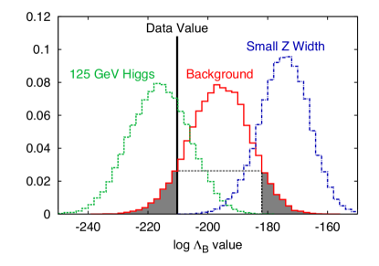
Figure 1: The unit normalized distribution of our test statistic, defined in Eq. (4) as evaluated for 20-event pseudoexperiments consisting of background $q\bar{q}\to 4\ell$ events (red solid curve), $gg\to H\to 4\ell$ signal events for a $125$ GeV Higgs (green dashed curve), and $q\bar{q}\to 4\ell$ events for which the $Z$ boson width has been reduced by a factor of $5$ (blue dot-dashed curve). If a particular value of our test statistic, indicated by “Data Value”, is observed, the corresponding $p$-value is given by the area in gray. In this specific case, $p\approx 0.13$.

How to Flatten Background Distributions: Examples.   The main point of this letter is that the procedure above allows one to exclude the background hypothesis in the presence of an unknown signal. In other words, one can confidently look for new physics models “away from the lamppost”, i.e., models which no theorist has yet thought of. While, in principle, any variable could have been used to construct such a test statistic, the use of a variable based on the background likelihood should additionally optimize the sensitivity of such searches.

We now present some related methods, which allow the “non-backgroundness” of some potential signal to be shown in a clear and intuitive way. These methods also have the benefit that they generalize to any possible channel, so results and sensitivity in various channels can easily be compared.

1.  Flattening with Ranking.   In this approach, one takes the normalized distribution, $\frac{dN}{d\xi}$, for some kinematic variable, $\xi$, and defines a “ranking” variable,

$$r(\xi)=\int_{-\infty}^{\xi}\frac{dN}{d\xi^{\prime}}d\xi^{\prime}.$$ (5)

We note that $r(\xi)$ is the cumulative distribution function for the background with respect to the variable $\xi$. We can now evaluate the ranking $r_{\xi}$ of any given event ${\mathcal{E}}$ by defining

$$r_{\xi}({\mathcal{E}})=r(\xi({\mathcal{E}})),$$ (6)

that is, the value of the ranking variable for a given event, ${\mathcal{E}}$, is the value found from Eq. (5) for the value of the kinematic variable $\xi$ obtained for the event. The connection between our ranking variable $r_{\xi}({\mathcal{E}})$ and the background $\xi$ distribution is shown pictorially in Fig. 2(a). The figure also illustrates the physical meaning of $r_{\xi}({\mathcal{E}})$ — it is the fraction of background events ${\mathcal{E}}^{\prime}$ in which $\xi({\mathcal{E}}^{\prime})<\xi({\mathcal{E}})$. If we then consider the normalized distribution of the background with respect to $r_{\xi}$, we find that

$$\frac{dN}{dr_{\xi}}=1,$$ (7)

hence the distribution of this variable for background events is flat, as is shown in Fig. 2(b). This procedure, of course, works for any kinematic variable, $\xi$, we especially recommend using it with the sensitive matrix-element-based variables advocated above. Thus, one obtains a sensitive variable for which the background distribution is flat, while the distribution of signal events is characterized by departures from flatness, as is also shown in Fig. 2(b).

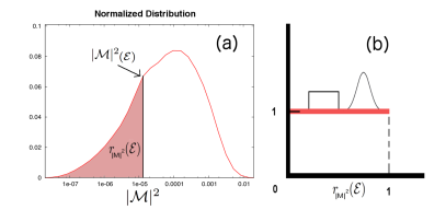
Figure 2: Panel (a) shows how the distribution of background MEKD for background events is used to create a “ranking variable”. In panel (b) we show that the background distribution with respect to this ranking variable is flat, while for other processes the distribution of background ranking variable is not flat.

We note in passing that calculating $r(\xi)$ from Monte Carlo (MC) events is quite straightforward. One simply calculates the value of the variable $\xi$ for each of the $N$ events in the MC sample, thus obtaining a list of values $\{\xi_{i}\}$. The value of $r(\xi)$ is then well-approximated by the fraction of the $\{\xi_{i}\}$ which are less than $\xi$, i.e.,

$$r(\xi)\approx\frac{1}{N}\sum_{i=1}^{N}\theta(\xi-\xi_{i}).$$ (8)

This procedure should facilitate the experimental implementation of this technique.

2.  Flattening with Quantile Bins.   An alternate approach is to use the method of quantile bins. If we are only considering one variable, $\xi$, this approach consists of finding $n+1$ values $\eta_{1},\eta_{2},...,\eta_{n+1}$ such that

$$\int_{\eta_{i}}^{\eta_{i+1}}\frac{dN}{d\xi}d\xi=1/n,$$ (9)

i.e., the integral of the distribution is equal in each bin. This procedure can be extended to the case where there are several variables $\xi_{i}$, where again we demand that the integral of the distribution be the same in each bin. For example, in two dimensions, we must choose values of $\xi_{1}$: $\eta_{1,1}$, $\eta_{1,2}$, …, $\eta_{1,n+1}$ and values of $\xi_{2}$: $\eta_{2,1}$, $\eta_{2,2}$, …, $\eta_{2,n+1}$, such that

$$\int_{\eta_{1,i}}^{\eta_{1,i+1}}\int_{\eta_{2,i}}^{\eta_{2,i+1}}\frac{d^{2}N}{d\xi_{1}d\xi_{2}}d\xi_{1}d\xi_{2}=\frac{1}{n^{2}}.$$ (10)

This procedure allows us to consider additional kinematic variables in addition to a likelihood-based variabe. Examples of this are shown in Figs. 3 and 4, in which we consider the distribution of four-lepton events at the 8 TeV LHC in terms of the four-lepton invariant mass, $m_{4\ell}$, and the background MEKD value.

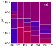
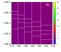
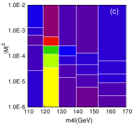
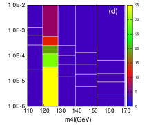
Figure 3: Quantile bins in $m_{4\ell}$ (x-axis) and $|{\mathcal{M}}|^{2}$ (y-axis) we constructed using the background ($q\bar{q}\to 2e2\mu$) distribution. We then plot the number of events in each quantile bin either from $150$ background $q\bar{q}\to 2e2\mu$ events (panels in the top row), or $75$ $125$-GeV Higgs signal and $75$ background events (panels in the bottom row). The panels in the left column are for one $150$ event pseudo-experiment, while the panels in the right column are for the average of $400$ pseudo-experiments.

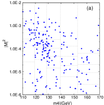
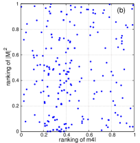
Figure 4: Simulated data consisting of $50$ 125-GeV Higgs $gg\to H\to 4\ell$ events and $150$ $q\bar{q}\to 4\ell$ events. In panel (a), the four-lepton invariant mass and pdf-weighted background squared matrix element have been plotted, while in panel (b) the ranking variable corresponding to these quantities, as defined in Eq. (5) is plotted. In each case, the dotted line mesh represents the quantile bin boundaries.

In Fig. 3 we show the results of an example experiment where we have formed quantile bins in $m_{4\ell}$ and $|{\mathcal{M}}|^{2}$, assuming the background hypothesis. We then plot the number of events in each quantile bin either from $150$ background $q\bar{q}\to 2e2\mu$ events (panels in the top row), or $75$ $125$-GeV Higgs signal and $75$ background events (panels in the bottom row). The panels in the left column are for one $150$ event pseudo-experiment, while the panels in the right column are for the average of $400$ such pseudo-experiments. Fig. 4 illustrates the same concept using scatter plots. Here the ratio of signal to background events has been changed from 1:1 (which is realistic for $125$ GeV $H\to 4\ell$ signal and the $q\bar{q}\to 4\ell$ background) to the much more challenging 1:3. Nevertheless, the presence of new signal can still be inferred from the anomalous clustering of points. Note that departures from uniform density are easier to interpret in the scatter plot in panel (b), which utilizes ranking variables.

3.  Flattening with Respect to All the Variables.   An extreme case of flattening the background distribution with respect to kinematic variables occurs when we consider a complete set of kinematic variables for some process. We can, of course, calculate the boundaries of these bins with Monte Carlo. However, in the limit where we have a good analytical, or at least numerical, understanding of the background, we can perform a flattening using the background distribution.

Specifically, if the background (after detector simulation, etc.) is described by the differential distribution $d^{n}N/d\bm{\xi}$, then if we weight each background event by $1/(d^{n}N/d\bm{\xi})$, we will end up with a distribution that is flat in the full $n$-dimensional space of values. If we weight data events according to this procedure, a signal will show up as deviations from flatness. This procedure is demonstrated in Fig. 5. The image in the top left represents our background PDF. If we generate “events” (i.e., pixels) according to this PDF, but weigh the corresponding 2D histogram by the reciprocal of the PDF, then we obtain an essentially flat distribution, shown in the top right corner. We now consider the bottom left image, where some “signal” (American football and flying saucers) have been added to the background. If events are generated according to this PDF, but weighted according to the reciprocal of the background PDF, we obtain the bottom right image, in which background features have been flattened, but signal features remain distinct.

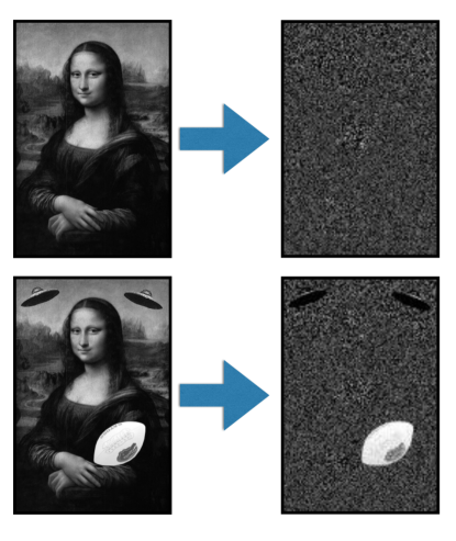
Figure 5: A demonstration of filling histograms with the reciprocal of the PDF for the case of background only (top row) and in the presence of both signal and background (bottom row).

Conclusions.  We have presented methods, which utilize variables based on the squared matrix element, to search for new physics signals at the LHC in a model independent way. These approaches allow for model-independent exclusions of the standard model in the presence of arbitrary, unspecified, new physics. We look forward to the utilization of such methods in the upcoming Run 2 at the LHC.

Acknowledgements. J.G. and K.M. would like to thank their CMS colleagues for useful discussions. All of the authors would also like to thank D. Kim and T. LeCompte for stimulating conversations and L. da Vinci for assistance with Fig. 5. Work supported in part by U.S. Department of Energy Grant DE-FG02-97ER41029.

References

- (1) L. Susskind, Phys. Rev. D 20, 2619 (1979); G. ’t Hooft, NATO Adv. Study Inst. Ser. B Phys. 59, 135 (1980).
- (2) J. R. Ellis, J. S. Hagelin, D. V. Nanopoulos, K. A. Olive and M. Srednicki, Nucl. Phys. B 238, 453 (1984); G. Jungman, M. Kamionkowski and K. Griest, Phys. Rept. 267, 195 (1996) [hep-ph/9506380]; G. Bertone, D. Hooper and J. Silk, Phys. Rept. 405, 279 (2005) [hep-ph/0404175].
- (3) K. Kondo, J. Phys. Soc. Jap. 57, 4126 (1988); K. Kondo, J. Phys. Soc. Jap. 60, 836 (1991); K. Kondo, T. Chikamatsu and S. H. Kim, J. Phys. Soc. Jap. 62, 1177 (1993); R. H. Dalitz and G. R. Goldstein, Phys. Rev. D 45, 1531 (1992); B. Abbott et al. [D0 Collaboration], Phys. Rev. D 60, 052001 (1999) [hep-ex/9808029]; J. C. Estrada Vigil, FERMILAB-THESIS-2001-07; M. F. Canelli, UMI-31-14921; V. M. Abazov et al. [D0 Collaboration], Nature 429, 638 (2004) [hep-ex/0406031]; J. S. Gainer, J. Lykken, K. T. Matchev, S. Mrenna and M. Park, arXiv:1307.3546 [hep-ph].
- (4) P. C. Bhat, Ann. Rev. Nucl. Part. Sci. 61, 281 (2011).
- (5) S. Chatrchyan et al. [CMS Collaboration], Phys. Lett. B 716, 30 (2012) [arXiv:1207.7235 [hep-ex]].
- (6) S. Chatrchyan et al. [CMS Collaboration], Phys. Rev. Lett. 110, 081803 (2013) [arXiv:1212.6639 [hep-ex]]; G. Aad et al. [ATLAS Collaboration], Phys. Lett. B 726, 120 (2013) [arXiv:1307.1432 [hep-ex]]; S. Chatrchyan et al. [CMS Collaboration], arXiv:1312.5353 [hep-ex].
- (7) Y. Gao, A. V. Gritsan, Z. Guo, K. Melnikov, M. Schulze and N. V. Tran, Phys. Rev. D 81, 075022 (2010) [arXiv:1001.3396 [hep-ph]]; S. Bolognesi, Y. Gao, A. V. Gritsan, K. Melnikov, M. Schulze, N. V. Tran and A. Whitbeck, Phys. Rev. D 86, 095031 (2012) [arXiv:1208.4018 [hep-ph]].
- (8) P. Avery, D. Bourilkov, M. Chen, T. Cheng, A. Drozdetskiy, J. S. Gainer, A. Korytov and K. T. Matchev et al., Phys. Rev. D 87, no. 5, 055006 (2013) [arXiv:1210.0896 [hep-ph]]. M. Chen, T. Cheng, J. S. Gainer, A. Korytov, K. T. Matchev, P. Milenovic, G. Mitselmakher and M. Park et al., Phys. Rev. D 89, 034002 (2014) [arXiv:1310.1397 [hep-ph]].
- (9) J. Neyman and E. S. Pearson, Phil. Trans. R. Soc. Lond. A 231 no. 694-706, 289-337 (1933).
- (10) J. Alwall, M. Herquet, F. Maltoni, O. Mattelaer and T. Stelzer, JHEP 1106, 128 (2011) [arXiv:1106.0522 [hep-ph]].
- (11) J. Heinrich, eConf C 030908, MOCT001 (2003) [physics/0310167]; R. Raja, physics/0509008.
- (12) N. Arkani-Hamed, G. L. Kane, J. Thaler and L. -T. Wang, JHEP 0608, 070 (2006) [hep-ph/0512190].