The rate, luminosity function and time delay of non-Collapsar short GRBs

Abstract

We estimate the rate and the luminosity function of short (hard) Gamma-Ray Bursts (sGRBs) that are non-Collapsars, using the peak fluxes and redshifts of BATSE, Swift and Fermi GRBs. Following Bromberg et al. (2013) we select a sub-sample of Swift bursts which are most likely non-Collapsars. We find that these sGRBs are delayed relative to the global star formation rate (SFR) with a typical delay time of a $3-4$ Gyr (depending on the SFR model). However, if two or three sGRB at high redshifts have been missed because of selection effects, a distribution of delay times of $\propto 1/t$ would be also compatible. The current event rate of these non-Collapsar sGRBs with $L_{iso}>5\times 10^{49}erg/s$ is $4.1_{-1.9}^{+2.3}Gpc^{-3}yr^{-1}$. The rate was significantly larger around $z\sim 1$ and it declines since that time. The luminosity function we find is a broken power law with a break at $2.0_{-0.4}^{+1.4}\times 10^{52}$ erg/s and power-law indices $0.95_{-0.12}^{+0.12}$ and $2.0_{-0.8}^{+1.0}$. When considering the whole Swift sGRB sample we find that it is composed of two populations: One group ($\approx 60\%-80\%$ of Swift sGRBs) with the above rate and time delay and a second group ($\approx 20\%-40\%$ of Swift sGRBs) of potential “impostors” that follow the SFR with no delay. These two populations are in very good agreement with the division of sGRBs to non-Collapsars and Collapsars suggested recently by Bromberg et al. (2013). If non-Collapsar sGRBs arise from neutron star merger this rate suggest a detection rate of 3-100 yr^-1 by a future gravitational wave detectors (e.g. Advanced Ligo/Virgo with detection horizon on 300 Mpc), and a co-detection with Fermi (Swift ) rate of 0.1-1 yr^-1 (0.02-0.14 yr^-1). We estimate that about $4\times 10^{5}(f_{b}^{-1}/30)$ mergers took place in the Milky Way. If $0.025m_{\odot}$ were ejected in each event this would have been sufficient to produce all the heavy r-process material in the Galaxy.

1 Introduction

GRB are divided into two distinct groups: long bursts with $T_{90}>2$ sec and short ones with $T_{90}<2$ sec (Kouveliotou et al., 1993). The short bursts are also typically harder than the long ones (Dezalay et al., 1996; Kouveliotou et al., 1996). Using the $\langle V/V_{max}\rangle$ test, Cohen & Piran (1995) have shown that the two populations are distributed differently in redshift space with the short GRBs being typically nearer to us, but still within cosmological distances. Afterglow detection in the late 90ies confirmed the cosmological origin of long GRBs and together with the discovery of SNe associated with the GRBs led to their identification as Collapsars. The origin of sGRBs remained obscure until 2005 when the HETE-2 and Swift satellites detected the first sGRB afterglows from GRBs 050509b, 050709 and 050724 (Bloom et al. 2006; D. B. Fox et al. 2006; Gehrels et al. 2005; Castro-Tirado et al. 2005b; Prochaska et al. 2005; Fox et al. 2005; Hjorth et al. 2005a, 2005b; Covino et al. 2006; Berger et al. 2005). This has led to the identification of the host galaxies. The difference between those hosts and the hosts of long bursts provided a strong indication that sGRBs result from a different type of physical progenitors (e.g. Berger, 2014; Fong et al., 2013; Nakar et al., 2006). When more sGRB redshifts have been accumulated the relatively low redshifts $\bar{z}\sim 0.5$ confirmed the earlier expectations, that were based just on the peak flux distribution, that the short bursts are nearer on average than the long ones (whose average redshift satisfies $\bar{z}>2$).

Recently Bromberg et al. (2013) have shown that the Swift sample of short ($T_{90}<2$ sec) bursts is contaminated by a significant fraction of short duration Collapsars (See however Fong et al., 2013, who seem to arrive to a different conclusion based on host morphologies). They have argued that due to its soft energy window Swift is less sensitive to the harder sGRBs and hence the division at $T_{90}=2$ sec found for BATSE bursts is inadequate for the Swift sample. They have estimated the probability that a given Swift short duration burst with a known duration and hardness is a non-Collapsar or that it is a short Collapsar. Bromberg et al. (2013) divide the bursts to subgroups according to their spectral index and estimate this probability as a function of the burst’s duration for each group separately. In this work we use this method to build a sample of non-Collapsars sGRBs in a way which minimizes the sample contamination by Collapsars and allows us to put a handle on the uncertainty associated with the sample contamination. Using this sample we explore the rate of non-Collapsar sGRBs and their luminosity function. We will refers in the rest of the text to this sample, so when we discuss sGRBs we actually mean non-Collapsar sGRBs, unless specified otherwise. We also explore the implication of using the full (contaminated sample) and we find that indeed the division, as suggested by Bromberg et al. (2013), is well justified.

The luminosity function and formation rate of sGRBs are fundamental to understanding the nature of these objects. It has been suggested (Eichler et al., 1989) that sGRB originate from neutron star-neutron star (ns²) or neutron star-black hole (nsbh) mergers. In this case we expect a delay between the SFR and the merger rate (Piran, 1992a; Ando, 2004) due to the time it takes for the binary orbits to spiral in. As such information about the rate could reveal the magnitude of this delay and provide a clue on the physics of the progenitor system, the relevant information goes beyond the physics of GRBs. The mergers end with a chirping burst of gravitational waves (GW) and gravitational detectors whose prime goal is to detect those signals are upgraded (LIGO, Virgo) or constructed (KAGRA) now. A major unknown factor in these observations is the expected rate of mergers within the detection horizon. The local sGRB rate is important for estimating of the detection rate of GW telescopes. Mergers are also a likely source of heavy r-process material (Lattimer & Schramm, 1974; Eichler et al., 1989). A crucial question is whether they can provide all heavy r-process material or is there another significant heavy r-process source. The major factor in answering this question is the overall rate of sGRBs. However, the variation of this rate with time is also important as some r-process material was produced very early on and an interesting question is whether mergers (that resulted also in GRBs) could have produced this material. Another important clue might be the recent discovery of macronova-like signature in GRB130603B (Tanvir et al., 2013; Berger et al., 2013).

There is a large sample of sGRBs detected by BATSE and by Fermi/GBM. However the redshifts of these bursts is unknown. The observed peak flux distribution of these bursts is a convolution of two unknown functions, the rate and the luminosity function and it is impossible to determine both functions without additional information. For example, Cohen & Piran (1995) have shown that the observed BATSE flux distribution can be fitted with very different luminosity functions depending on the choice of the GRB rate and vice versa. Furthermore, Nakar et al. (2006) has shown that for a single power law the peak-flux distribution will also be a power law and it will not depend on the formation rate of the GRBs. Since the BATSE peak-flux data is indeed consistent with a single power law luminosity function we cannot use it to constrain the formation rate.

We resolve this problem by combining the small Swift (Gehrels et al., 2004) sGRB redshift sample with the large sGRB samples of BATSE and Fermi. We carry out a combined likelihood analysis using the BATSE and the Fermi/GBM peak flux distributions and the Swift sGRB redshift sample. The combined sample enables us to constrain both the rate of sGRB and the luminosity function. In §2 we define the samples and discuss possible selection effects. We define in §3 models for the luminosity function and the rate, considering a time delay with respect to the SFR. We also build the likelihood function and describe the method to determine the most probable parameters for the rate and the luminosity function and their associated uncertainty range. In §4 we present the results of the analysis for the different models and finally in §5 we discuss the results and their implications on the progenitors of sGRBs and on the detection rate of gravitational waves. We also discuss the consistency of our results with the predicted fraction of Collapsars and non-Collapsars suggested by Bromberg et al. (2013).

2 The samples

We jointly analyze here observations from three major GRB targeted missions: BATSE, Swift and Fermi. We stress that there is no single standard way to jointly analyze the observations of the different detectors having different energy bands and different triggering scheme. We must make certain assumptions to allow such joint analysis: first we define a threshold for the duration for each detector’s sample in a consistent way. Obviously setting the same value of $T_{90}$ threshold for all detectors does not serve this goal since the $T_{90}$ are defined differently on the detectors ($T_{90}$ is defined for the energy bands [50-300]keV, [15-150]keV and [50-300]keV for BATSE, Swift and Fermi respectively). A more consistent way would be taking a uniform threshold value of $f_{NC}$ for all detectors i.e. taking only bursts which are more likely to be a non-collapsars (e.g. $f_{NC}>$ 0.6, as we used for Swift ).

Our samples consist of short BATSE and Fermi bursts with a measured peak-flux and of Swift short bursts with redshift. Following Bromberg et al. (2013) we estimate the level of contamination of the sample by Collapsars events. For the BATSE and Fermi we adopt the traditional duration cutoff $T_{90}<2$ sec as it yields a low contamination of Collapsars in the sample at the $10\%-15\%$ level. For the Swift sample a duration cutoff of $T_{90}<2$ sec would yield a contamination fraction of $32\%$, hence we adopt the more sophisticated selection method using both the duration and the spectral index of the bursts. We include bursts for which the probability of being non-Collapsar is $>0.6$. This results in a sample of 12 bursts with an estimated contamination fraction of only $7\%$ i.e. only one of these bursts is expected to be an impostor (see table 2.2 for the sample). The contamination fractions for the different detectors are comparable (10%, 15%,7%). The use of different contamination fractions has no impact on the major results in this paper.

There are number of selection effects concerning the peak-flux and the redshift samples (see Coward et al., 2013, for a review). We minimize the biases that arise from the detectors’ sensitivity limit by selecting a high flux limit for BATSE and Fermi bursts. The Swift redshift sample is small and hence we use the whole sample, therefore it is susceptible to the biases described in Coward et al. (2013). We caution though that if the lack of higher redshift ($z>1.2$) non-Collapsar sGRBs is a result of an observational bias some of our conclusions concerning the delay between the sGRBs and the SFR (see §5.) might be significantly weakened. In particular we discuss later a case in which a few bursts at $z>1.2$ are artificially added to the sample and check its implications.

2.1 The BATSE and Fermi Flux samples

Following Nakar et al. (2006) we extract from the current BATSE catalog all short ($T_{90}<2$ sec) bursts with a peak flux in the 64 ms timing window of $P_{64}>1.5$ [ph/cm² sec], yielding a sample of 341 bursts. The duration $T_{90}=2s$ corresponds to a non-Collapsar probability of 0.6, and the expected fraction of non-Collapsar in the entire sample is 0.9.

We take the short ($T_{90}<2$ sec) bursts with a peak flux in the 64 ms timing window (and in the [50keV - 300keV] energy band) of $P_{64}>2.37$ [ph/cm² sec] from the Fermi GBM Burst Catalog (Paciesas et al., 2012a, b) until date 10-April-2013. This yields a sample of 145 bursts. The flux threshold is estimated by comparing the peak-flux distribution with that of BATSE. Consistent with the findings of Nava et al. (2011) the Fermi threshold is higher than the BATSE threshold. $T_{90}=2$ sec corresponds to a non-Collapsar probability of 0.45, and the expected fraction of non-Collapsar in the entire sample is 0.85.

2.2 The Swift Redshift sample

The entire Swift sGRBs redshift sample consist of 20 short ($T_{90}<2$ sec) Swift bursts which have a redshift determination. We did not include bursts that have a short peak followed by an extended emission with overall $T_{90}>2$ sec. The $T_{90}$ duration and the 1-sec peak-flux are taken from the Swift mission page. The 64-ms peak-flux of the bursts was estimated by correcting the 1-sec peak-flux with the ratio of the 64-ms and 1024-ms peak-counts in the 64-ms binned light-curve provided in Swift Burst Ground-Analysis Information page (Barthelmy et al., 2005; Sakamoto et al., 2008; Sakamoto et al., 2011). The probability of a burst being a non-Collapsar is calculated following Bromberg et al. (2013). Table 2.2 lists, for the Swift bursts sample, the redshift, peak-flux, luminosity, duration, photon index and $f_{NC}$ - the probability for being a non-Collapsar. From this sample we select a subgroups of 12 events with a high probability for being non-Collapsars ($f_{NC}>0.6$) to establish a “genuine” redshift sample on which we carry most of the analysis. We will return to the full sample in §3.2 and establish that it is indeed more compatible with a bimodal distribution of event rates.

The Peak-flux threshold alone is a very rough estimate for the Swift GRB detection threshold (see e.g. Lien et al., 2014) as the actual detection as well as redshift determination depend on many factors. Nonetheless we have estimated the Swift detection threshold for sGRB with redshift measurement roughly as $P_{lim}=2.5ph/s/cm^{2}$. We have repeated the analysis for other values of $P_{lim}$ and found that the luminosity function and the rate do not change significantly. However, the expected luminosity distribution and redshift distribution are consistent with the observations only for $P_{lim}\simeq 2.5$.

GRB	z	Ref.	$P_{64}$	$L_{51}$	$T_{90}$	$P.L.$	$f_{NC}$
050509B	0.225	1	1.32	0.22	0.07	1.57	0.87
060502B	0.287	2	3.24	0.89	0.13	0.98	0.99
060801	1.131	3	4.09	16.14	0.49	0.47	0.95
061201	0.111	4	10.46	0.42	0.76	0.81	0.92
061217	0.827	5	6.73	14.81	0.21	0.86	0.98
071227	0.383	6	4.99	2.44	1.80	0.99	0.71
080905A	0.122	7	4.63	0.23	1.00	0.85	0.88
090510	0.903	8	46.75	121.4	0.30	0.98	0.97
100117A	0.920	9	11.14	29.95	0.30	0.88	0.97
100206A	0.407	10	11.91	6.56	0.12	0.63	0.99
101219A	0.718	11	12.01	20.16	0.60	0.63	0.94
130603B	0.356	12	47.30	20.01	0.18	0.82	0.99
Average	0.532		13.71	19.44	0.50	0.87	0.93

050813^a 1.8^a 13 4.65 42.10^a 0.45 1.28 0.57 051221A 0.547 14 45.84 45.33 1.40 1.39 0.18 070429B 0.904 15 7.20 18.73 0.47 1.72 0.32 070724A 0.457 16 3.06 2.12 0.40 1.81 0.37 070809 0.219 17 2.62 0.42 1.30 1.69 0.09 090426 2.609 18 5.16 87.84 1.20 1.93 0.10 100724A 1.288 19 4.14 20.72 1.40 1.92 0.08 131004A 0.717 20 6.73 11.27 1.54 1.81 0.29 Average 0.933 9.93 24.29 1.02 1.69 0.25 Total Avg. 0.693 12.20 21.38 0.71 1.20 0.66

Table 1: The Swift sGRBs redshift sample: Swift bursts with $T_{90}\lesssim 2$ sec and a measured redshift. The top part includes the bursts with $f_{NC}>0.6$ and the bottom part includes the bursts with $f_{NC}\leq 0.6$. $P_{64}$ is the 64-ms peak photon flux in $ph\ s^{-1}cm^{-2}$ in the Swift energy band [15keV - 150keV]; $L_{51}$ is the peak luminosity in $10^{51}erg/s$ (see text for the detailed definition); $T_{90}$ is the observed burst duration in seconds; $P.L.$ is the spectral photon power-law index in the Swift energy band [15keV - 150keV]; $f_{NC}$ is the probability that this bursts is a non-collapsar (genuine sGRBs) given the burst’s duration and its photon power-law index. (a) Two possible redshifts are suggested for the burst 050813: 1.8 and 0.722. We list the first in the table with the corresponding luminosity and refer to the sample as full sample (A). The corresponding luminosity for this burst at z=0.722 is $7.89\times 10^{51}$ erg/s and the sample with these values for that bursts is refered to as full sample (B). Redshift references: (1) Prochaska et al., 2005; Gehrels et al., 2005; (2) Bloom et al., 2006; (3) Cucchiara et al., 2006; (4) Berger, 2006a, 2007; (5) Berger, 2006b; (6) D’Avanzo et al., 2007; Berger et al., 2007; (7) Rowlinson et al., 2010; (8) Rau et al., 2009; (9) Fong et al., 2011; (10) Cenko et al., 2010; (11) Chornock & Berger, 2011; (12) Thone et al., 2013; Foley et al., 2013; Sanchez-Ramirez et al., 2013; Cucchiara et al., 2013; Xu et al., 2013; (13) Gehrels et al., 2005; Berger, 2005; Foley et al., 2005; (14) Berger & Soderberg, 2005; Soderberg et al., 2006; (15) Perley et al., 2007; (16) Cucchiara et al., 2007; Covino et al., 2007; (17) Perley et al., 2008; (18) Levesque et al., 2009; Thoene et al., 2009; (19) Thoene et al., 2010; (20) Chornock et al., 2013; D’Elia et al., 2013.

3 Methods

We construct models for the luminosity function and the rate and estimate the likelihood for obtaining the observed data given these models. By maximizing the likelihood, we obtain the best fit parameters for the different models. We estimate, using the likelihood function and Monte Carlo simulations the errors in these parameters.

3.1 The models

The models are a functional forms for the luminosity function and for the rate. For the luminosity function we chose the standard broken power law used when considering GRBs:

$$\phi_{0}(L)=\left\{\begin{array}[]{ll}(\frac{L}{L^{*}})^{-\alpha_{L}}&L<L^{*}\ ,\\ (\frac{L}{L^{*}})^{-\beta_{L}}&L>L^{*}\ .\end{array}\right.$$ (1)

This luminosity function is the logarithmic luminosity function defined as the (un-normalized) fraction of bursts within a logarithmic interval $d\log(L)$. The “linear“ luminosity function is related to the logarithmic one by incrementing $\alpha_{L}$ and $\beta_{L}$ by 1. We designate this general model as a broken power-law when $\alpha_{L}$, $\beta_{L}$ and L* are free parameters. We wish to examine the significance of the break in the luminosity function by also considering a model with a single power law luminosity function. By comparing the likelihood of the models, we show later, at the results section, that a broken power law is significantly preferred over a single power law for modeling the luminosity function.

We define the 64-ms isotropic-equivalent peak luminosity $L$ in the [1keV - 10MeV] energy band by assuming an average Band-function (Band et al., 1993) for all bursts using the typical parameters of the Band function for Fermi/GBM (Nava et al., 2011): $E_{peak}$ = 800 keV (in the source frame ), $\alpha_{BAND}=-0.5$, $\beta_{BAND}=-2.25$. Note that this definition of the luminosity give luminosities which are larger by a factor of $3-10$ - depending on the redshift and on the detectors’ energy window - compared with the luminosity in the “classical” energy band ($50keV-300keV$ as in e.g. Guetta & Piran, 2006). The peak luminosity is related to $P$, the 64-ms peak photon count as:

$$L=4\pi D(z)^{2}(1+z)k(z)C_{det}~{}P\ ,$$ (2)

where $D(z)$ is the proper distance at redshift $z$. $C_{det}$ (having units of energy) is the total $\gamma$-ray luminosity divided by the number rate of photons in the detector’s energy window from a source at redshift = 0:

$$C_{det}=\frac{\int_{1keV}^{10MeV}EN(E)dE}{\int_{E_{min}}^{E_{max}}N(E)dE}\ .$$ (3)

Finally, $k(z)$ is the k-correction for the given spectrum at redshift z,

$$k(z)=\frac{\int_{E_{min}}^{E_{max}}N(E)dE}{\int_{(1+z)E_{min}}^{(1+z)E_{max}}N(E)dE}\ ,$$ (4)

where $N(E)$ is the Band function and $[E_{min},E_{max}]$ is the detector’s energy window.

With the ns² merger model in mind we construct a rate function that describes a rate that has a time delay (corresponding to the spiral-in time of the binaries) relative to the global SFR. Such a rate is given as a convolution of a given selected SFR (we consider in the following two SFR functions) and a time delay, $\Delta t$, with a distribution, $f(\Delta t)$, relative to the SFR. We stress that while motivated by the ns² model we allow for the possibility of no time delay at all and let the maximal likelihood procedure find the best fit values. Thus, we do not force the ns² model on the data. The intrinsic sGRB rate is a convolution of the SFR with $f(\Delta t)$:

$$R_{sGRB}(z)\propto\int_{z}^{\infty}{SFR(z^{\prime})(f(t(z)-t(z^{\prime}))\frac{dt}{dz^{\prime}}dz^{\prime}}\ .$$ (5)

We consider two models for the time delay: I. A power-law time delay with index $\alpha_{t}$ and a minimum time delay of $20Myr$: $f(\tau)=\tau^{-\alpha_{t}}$ for $\tau>20Myr$. Note that the simple ns² merger model favors $\alpha_{t}=1$ (Piran, 1992a). At the limit $\alpha_{t}\rightarrow\infty$, $R_{sGRB}$ tends to the SFR and the model is almost indistinguishable from the SFR for $\alpha_{t}>3$ . II. A log-normal distribution with a width $\sigma_{t}$ around a time delay $t_{d}$: $f(\tau)=\exp[{-\frac{(\ln\tau-\ln t_{d})^{2}}{2\sigma_{t}^{2}}}]/({\sqrt{2\pi}\sigma_{t}})$. For small values of $\sigma_{t}$ this function converges, of course, to a constant time delay. Hereafter we refer to that limit as the constant time delay model. In some cases we will consider this case in the analysis.

We examine two SFR models: (i) We combine the low redshift SFR of Cucciati et al. (2012) with the high redshift part ($z>4$) of Bouwens et al. (2012) and Oesch et al. (2013) (We denote this as SFR1). The lower redshift part of this SFR is measured using the VIMOS-VLT Deep Survey (VVDS), a single deep galaxy redshift survey (Cucciati et al., 2012) up to redshift $z\sim 4.5$. The higher redshift part is derived from the UV LFs from the Hubble ultra-deep WFC3/IR data (We used the compilation in Oesch et al., 2013). (ii) The Planck Collaboration et al. (2013) Halo model (denoted SFR2). This is based on a completely different method which estimates the SFR from the cosmic infrared background (CIB) anisotropies measured with Planck. This method is based on a model that associates star-forming galaxies with dark matter halos and their sub-halos, using a parametrized relation between the dust-processed infrared luminosity and (sub-)halo mass. SFR2 is not expected to be very accurate for $z>2$, nevertheless these two SFR models represent a range of feasible SFR models which allow us to estimate the sGRBs rate time delay with respect to different SFRs. The two SFR models are plotted in figure 1, together with few other commonly used SFR models.

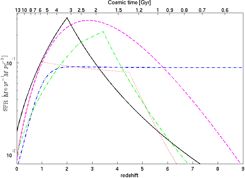
Figure 1: The star formation rate models vs. redshift. Cucciati et al. (2012) (SFR1) - black solid line, Planck Collaboration et al. (2013) Halo model (SFR2) - magenta dashed line. Three other commonly used SFRs which we do not use are plotted here to emphasize the range of SFRs in the literature: Porciani & Madau (2001) SF2 model - blue dash-dotted line, Bouwens et al. (2011) - green dashed line (peaks at redshift $\sim 3.4$) and Hopkins & Beacom (2006) piecewise linear model - red dotted line (almost flat in the redshift range $1-4.4$).

3.2 A two component analysis

We have asserted, following Bromberg et al. (2013), that Swift sGRBs are composed of two populations, one of genuine non-Collapsars and the other of “impostor” namely short Collapsars. To explore and demonstrate this assertion we have incorporate another model that allows for two populations that have different event rates. The two populations have the same luminosity function, as the sample is not large enough to explore two different luminosity functions at the same time. One of the two populations has a time delay relative to the SFR, while the other one follows the SFR with no delay. The free parameter $f_{SFR}$ determines the relative fraction of these two components:

$$R(z)=(1-f_{SFR})\cdot R_{sGRB}(z)+f_{SFR}\cdot SFR(z),$$ (6)

where $R_{sGRB}(z)$ is given by equation 5. If our assertion is correct we expect that when applying this rate model to the full Swift sample $f_{SFR}$ will obtain the fraction of non-Collapsar that is determined using other methods (combination of duration of hardness). This will demonstrate that indeed it is composed of two distinct populations (see §4).

3.3 The likelihood function

The likelihood function, $\cal L$, describes the combined likelihood of observing the BATSE, Fermi and Swift data:

$$\begin{split}{\cal L}=\prod_{i}^{BATSE}\left(\frac{N^{\prime}(P_{i})}{\int_{P_{min}^{BATSE}}^{P_{max}^{BATSE}}N^{\prime}(P)dP}\right)\prod_{j}^{Fermi}\left(\frac{N^{\prime}(P_{j})}{\int_{P_{min}^{Fermi}}^{P_{max}^{Fermi}}N^{\prime}(P)dP}\right)\\ \prod_{k}^{Swift}\left(\frac{\phi_{0}(L_{k})R_{sGRBs}(z_{k})}{\int_{P_{min}^{Swift}}^{P_{max}^{Swift}}N^{\prime}(P)dP}\right),\end{split}$$ (7)

where the product is over all bursts in the BATSE (i), Fermi (j) and Swift (k) samples. The observable number density for a peak flux $P$ is given by:

$$N^{\prime}(P)=\frac{1}{P}\int_{0}^{\infty}R_{sGRBs}(z)\phi_{0}(L(z,P))dz,$$ (8)

where $L(z,P)$ is given by equation 2.

The best-fit parameters are found by maximizing the likelihood over the parameter space for each parameter or by marginalizing the likelihood over of the sub-space of all the other parameters. In all cases the best-fit parameters do not significantly differ whether maximizing or marginalizing the likelihood. The uncertainty range is estimated using the likelihood ratio where $1\sigma$ (68%) uncertainty level corresponds to a likelihood ratio of $e^{-0.5}$. The above uncertainty level estimation is validated by a Bootstrap Monte-Carlo simulation. We note that this might be a poor estimator in cases where the maximum value of the likelihood is found at the edge of the parameter space as in the case of the width of the log-normal distribution for time delay. The local event rate $\rho_{0}$ is found by comparing the total expected number of events from the maximum likelihood model to the total observed BATSE and Fermi sGRBs and correcting for the non-Collapsars fraction of all burst with $T_{90}>2s$ following Bromberg et al. (2013). By performing this calculation for all points in the parameter space for which the likelihood ratio is above $e^{-0.5}$ we get a range of $\rho_{0}$ values which is the estimated $1\sigma$ uncertainty range of $\rho_{0}$.

4 Results

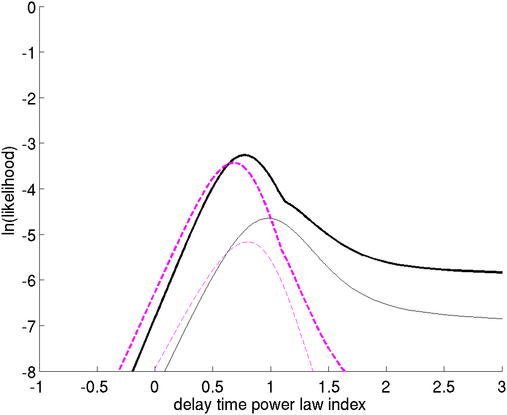
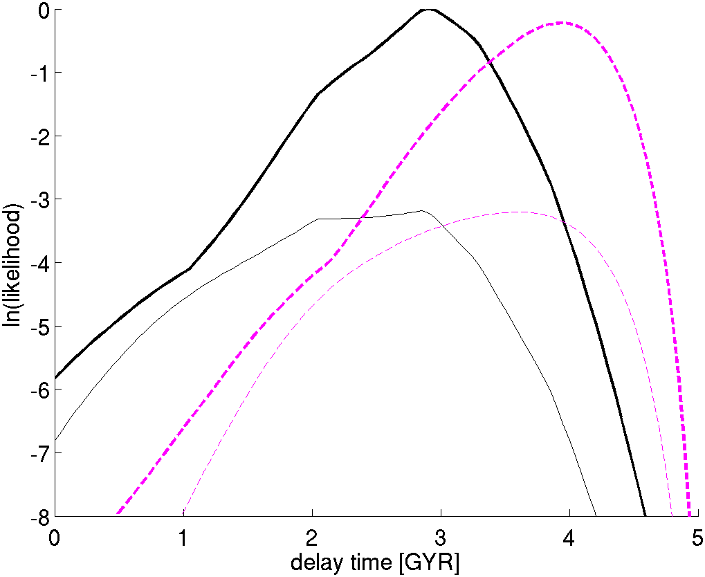
Figure 2: The maximum likelihood as a function of the power law time delay parameter $\alpha_{t}$ (Top panel) / constant time delay parameter $t_{d}$ (Bottom panel) - all are normalized by the maximum likelihood of the highest model. The line color and shape denote the SFR model: SFR1 - black solid line, SFR2 - magenta dashed line. Each of the SFRs have two lines in each panel: the upper-thick line is for a broken power-law luminosity function model and the lower-thin line is for the single power-law luminosity function model.

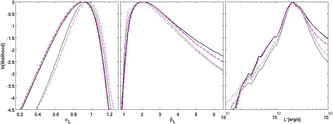
Figure 3: The marginalized likelihood ratio as a function of each the luminosity function parameters $\alpha_{L}$, $\beta_{L}$ and $L*$ (for the three panels from left to right). The line color and shape denote the SFR model: SFR1 - black solid line, SFR2 - magenta dashed line. Each of the SFRs have two lines: the thin line is for a power-law time delay model and the thick line is for the constant time delay model (each model is normalized separately).

Figure 4: Contours of the log-likelihood as a function of the time delay in Gyr and the standard deviation of the time delay log-normal distribution. Left hand side panel: SFR1, right hand side panel: SFR2. The contour levels represent a factor of $e^{0.5}$ in likelihood between two adjacent lines.

Figure 5: Contours of the maximum log-likelihood as a function of the time delay parameter and the SFR fraction for the ’two time delay components’ model. The different panels are for the two SFR models we study and for the sub-samples of bursts with redshifts: Left hand side panels: SFR1, right hand side panels: SFR2, top and middle panels: for all 20 bursts for burst 050813 at z=1.8 and z=0.722 respectively, bottom panels: for the 12 bursts with $f_{NC}>0.6$. The contour levels represent a factor of $e^{0.5}$ in likelihood between two adjacent lines.

Our results are shown in Figures 2 - 5. Figure 2 depicts the maximum likelihood as a function of the delay power-law index or of the time delay (the latter for the constant time delay model). Figure 3 depicts the likelihood for each of the parameters of the broken power-law luminosity function. Figure 4 depicts the likelihood contours in the log-normal distribution parameter space (delay time $t_{d}$ - delay width $\sigma_{t}$) and Figure 5 depicts the likelihood contour lines for the SFR fraction parameter, $f_{SFR}$, of the two component model (both for the full sample analysis and for the non-collapsars sub-sample). We present the results as curves of the likelihood as a function of different parameters. Figure 2 depict the maximal likelihood for the given parameter shown in the figure where we scan the phase-space of the rest of the model parameters. This enables us to compare different parameter spaces, i.e. a single power-law and a broken power-law models for the luminosity function. Figures 3 - 5 depict the marginalized likelihood for the given parameter(s) shown in the figure over the phase-space of the rest of the model parameters. The results of the maximal likelihood in all cases are very similar to the results of marginalizing the likelihood, thereby confirming the robustness of the result. The most likely value and uncertainty range (after marginalization) for each parameter are summarized in Table 2. Also reported in Table 2 are the likelihood ratios, namely the ratios of the maximal likelihood in a given model and the maximal likelihood among all four models examined. This enables us to compare between the different models.

The likelihoods for the single power-law luminosity function and the broken power-law luminosity function are shown in figure 2. The likelihood for the broken power-law model is higher than likelihood for the single power-law model by a factor $3-4$ which corresponds to a rejection of the single power law model at $\sim 2.5\sigma$. We adopt, therefore, the more general broken power-law luminosity function for the rest of the analysis.

Figure 2 depicts the likelihood for the two SFRs and for the two time delay distributions. For both SFR models when considering the power-law time delay distribution $\alpha_{t}$, the time delay power law index peaks around $0.7-0.8$. This is consistent with the value 1, expected for a distribution that arises from mergers Piran (1992b). However for both SFR models the maximal likelihood of the constant time delay model (or the log-normal distribution) was significantly higher than the maximum likelihood of the power-law time delay model. This means that the power law delay time model is disfavoured as describing the rate of sGRB. The power-law delay time model predicts a significant fraction sGRBs with short delays and hence a significant fraction of $z\gtrsim 1$ bursts while the log-normal time delay model successfully suppress the $z\gtrsim 1$ population and is consistent with the observed redshift distribution. From all our results this result, which has important physical implications that we discuss later, is most sensitive to observational bias. In particular this conclusion strongly depends on the observed redshift sample and it depends critically on the lack of $z>1.2$ bursts in our non-Collapsar sGRB sub-sample. Note that among the likely Collapsars sGRBs that we have eliminated from our sample there are a few bursts above this redshift. A detection of two or three non-Collapsar sGRBs with a higher redshift may change this conclusion.

The likelihood of the constant time delay model peaks at $2.9$ Gyr and $3.9$ Gyr for SFR1 and SFR2 respectively. This time delay ranges from $2.5$ Gyr to $3.3$ Gyr for SFR1 and from $3.4$ Gyr to $4.3$ Gyr for SFR2. Figure 4 depicts the likelihood contours for the log-normal model as a function of the average time delay and the spread around this average. The likelihood peaks (for both SFRs) at zero width i.e. at a constant time delay. The width of the log-normal distribution is $\sigma_{t}\lesssim 0.2$ (at 68% confidence), which corresponds to a very small spread by a factor of $\lesssim 1.2$ in the time delays. As a constant time delay gives the best fit we adopt it throughout the paper, replacing the more general log-normal distribution.

As mentioned earlier it is possible that some burst at $z>1.2$ are missed because redshift measurements in this range are harder, as their main spectral lines leave the optical band. To study the effect of such bias on the main result of the paper - the preferred time delay model - we have simulated sets of redshift samples by adding a varying number of bursts uniformly distributed in the redshift range $1<z<2$ to our observed sample of 12 non-collapsars sGRBs, and have randomly drawn the luminosity from the luminosity function we get for the real sample, taking only the part which is above the detector’s threshold for the given redshift. We have repeated the analysis of the resulted likelihood function for each simulated redshift sample and specifically looking on the likelihood ratio between the log-normal and the power-law time delay models. The conclusion is that by adding 2-3 bursts in the $1<z<2$ redshift range we void the preference of the log-normal time delay model making both model consistent with the simulated samples. Adding further more bursts at that redshift range does not change this, as the parameters of each of the time delay models vary but they are both consistent as no model can be said to be significantly more likely than the other.

Once we have figured out the parameters for the “uncontaminated” Swift sample we turn to examine the whole sample of Swift sGRBs with redshifts (still excluding sGRBs with long soft tails). In this case, as mentioned earlier in §3.2, we have modeled the sGRB rate as as sum of two components, one with a constant time delay and the other with no time delay relative to the SFR. The ratio of these two components is not set a priori and it is a new free parameter, which we denote as the “SFR fraction” $f_{SFR}$. We carry out this analysis twice. Once, on the full Swift sample (20 bursts) and once as a check on the uncontaminated sample from which we have kept only Swift sGRBs that have high probability of being Collapsars (12 bursts). The full sample itself has two variants because the redshift of burst 050813 may be either 1.8 or 0.722. These two options are referred to as “full sample (A)” and “full sample (B)” respectively.

Figure 5 depicts contours of the likelihood as a function of the time delay parameter $t_{d}$ and the “SFR fraction” $f_{SFR}$ for the two SFR models that we consider and for the two samples. The best-fit values and the $1\sigma$ uncertainty ranges are summarized in Table 3. As expected the maximal likelihood for the uncontaminated sample arises when all bursts have a delay (the “SFR fraction” vanishes) and in this case we recover the delay times derived earlier. On the other hand once we consider the full sample we find that the maximal likelihood is obtained for $f_{SFR}=0.30_{-0.15}^{+0.18}$ for the full sample (A) and $f_{SFR}=0.18_{-0.12}^{+0.17}$ for the full sample (B) with SFR1 and $f_{SFR}=0.20_{-0.10}^{+0.15}$ for the full sample (A) and $f_{SFR}=0.11_{-0.07}^{+0.13}$ for the full sample (B) with SFR2. This number is to be compared with the fraction of Collapsars in the full sample which can be read from the last line in Table 2.2 $f_{C}=f_{Collapsar}=1-f_{Non-Collapsar}$ = 0.34. The $f_{SFR}$ values for both SFR models are significantly inconsistent with zero but they are consistent with $f_{C}$ of the full sample, providing an independent evidence that Swift short GRBs contain a significant fraction of short Collapsars (Bromberg et al., 2013). One cannot rule out, of course, the possibility that all bursts are genuine non-Collapsars and that there is a population of non-Collapsars sGRBs that follows the SFR without time delay. Such a possibility has been found in some population synthesis models (Belczynski et al., 2002).

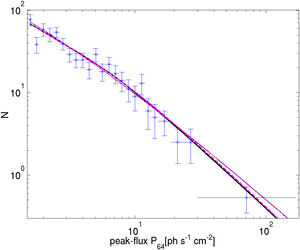
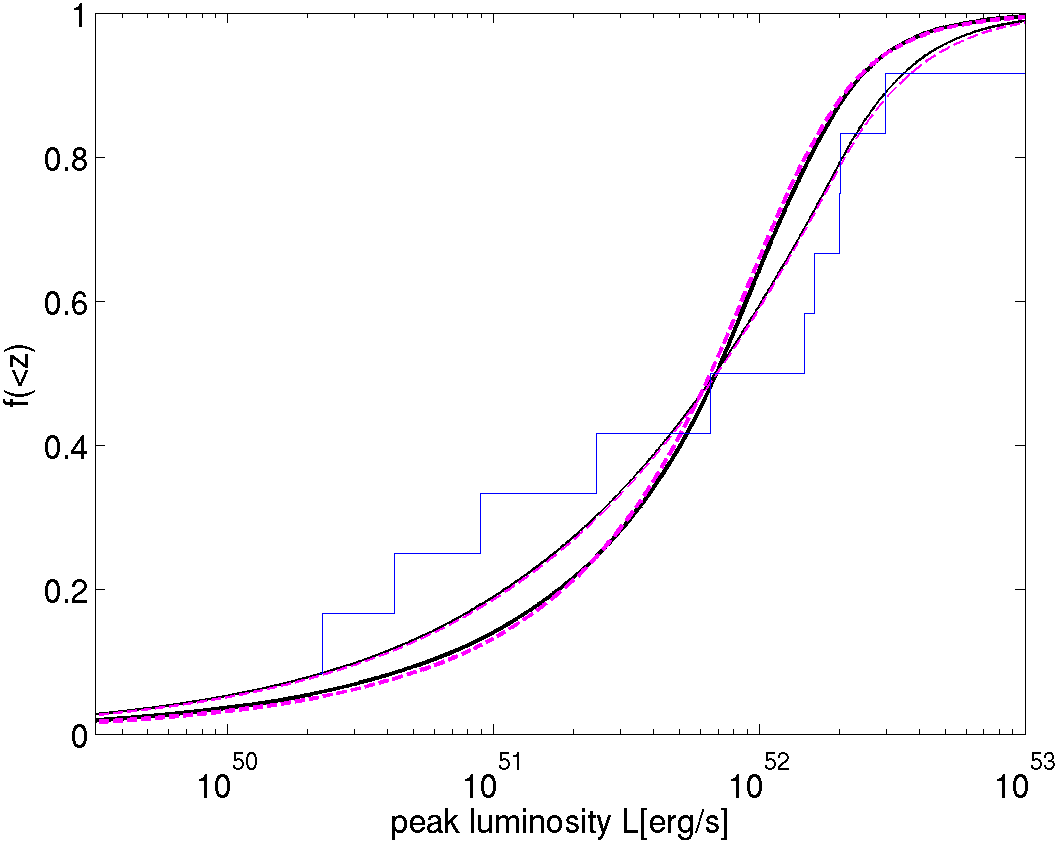
Figure 6: Top panel: peak-flux distribution and the models found for BATSE and Fermi together (see text for details). The modeled peak-flux distributions are consistent with the observed sample: $\chi^{2}=19.4,19.7,21.0$ and $21.0$ (d.o.f.=23) for the log-normal time delay model with SFR1 or SFR2, and the power-law time delay model with SFR1 or SFR2, respectively. Bottom panel: the observed (12 bursts with $f_{NC}>0.6$) and the predicted luminosity cumulative distribution for the log-normal time delay model (thick lines) and the power-law time delay model (thin lines). For both the peak-fluxes and the luminosity distributions, the black solid line and the magenta dashed line corresponds to SFR1 and SFR2 respectively. The modeled luminosity distributions are not inconsistent with the observed sample: $P_{KS}=0.24,0.19$ for the log-normal time delay model with SFR1, SFR2 and $P_{KS}=0.64,0.67$ for the power-law time delay model with SFR1, SFR2.

Figure 7: Top panel: The SFRs - (black dashed-dotted and magenta dotted lines for SFR1 and SFR2 respectively) and the sGRB rates for the log-normal time delay models (thick solid and thick dashed lines) and the power-law time delay model (thin solid and thin dashed lines). Bottom panel: The observed (12 bursts with $f_{NC}>0.6$) and the predicted redshift cumulative distribution for the log-normal time delay model (thick lines) and the power-law time delay model (thin lines). For both panels, the black solid line and the magenta dashed line corresponds to SFR1 and SFR2 respectively. The modeled redshift distributions are not inconsistent with the observed sample: $P_{KS}=0.36,0.34$ for the log-normal time delay model with SFR1, SFR2 and $P_{KS}=0.63,0.62$ for the power-law time delay model with SFR1, SFR2.

As a demonstration of the quality of the fit we compare the predictions of the model for BATSE, Fermi and Swift with the observations. Figure 6 and Figure 7 compare the observed samples of BATSE, Fermi and Swift with the best-fit models of both a constant time delay and a power law time delay with SFR1 and SFR2. For the peak-flux distribution we have used the effective full sky observing time of BATSE and Fermi i.e. observations period times the field of view (4.44 yr for BATSE and 3.65 yr for Fermi), and corrected accordingly the first four bins with peak-flux $<2.37ph~{}cm^{-2}s^{-1}$ where we have only BATSE bursts in our sample. We obtain good fits for the models (we denote here the results corresponding the two SFR models in the format [SFR1;SFR2]) with $\chi^{2}/d.o.f.=[21.4/19;21.4/19],[15.3/12;15.5/12]$ and $[19.4/23;19.7/23]$ for BATSE, Fermi and both, respectively for the constant time delay model and $\chi^{2}/d.o.f.=[22.7/19;22.7/19],[16.7/12;16.6/12]$ and $[21.0/23;21.0/23]$ for BATSE, Fermi and both, respectively for the power law time delay model. We have also tested the luminosity and redshift distributions of our Swift sample using a Kolmogorov-Smirnov (KS) test. For the constant time delay model we find a KS probabilities of $[0.24;0.19]$ and $[0.36;0.34]$ for the luminosity and redshift distributions respectively. We find KS values of $[0.64;0.67]$ and $[0.63;0.62]$ for the luminosity and redshift distributions respectively for the power law time delay model.

time delay model	log-normal	log-normal	power-law	power-law
SFR model	SFR1	SFR2	SFR1	SFR2
likelihood ratio	1	0.801	0.038	0.032
$\rho_{0}$ [$Gpc^{-3}yr^{-1}$]	$4.6_{-1.7}^{+1.9}$	$3.6_{-1.4}^{+1.6}$	$7.8_{-4.5}^{+5.1}$	$7.7_{-4.6}^{+5.4}$
$\alpha_{L}$	$0.94_{-0.13}^{+0.11}$	$0.96_{-0.12}^{+0.11}$	$0.91_{-0.17}^{+0.11}$	$0.90_{-0.17}^{+0.12}$
$\beta_{L}$	$2.0_{-0.7}^{+1.0}$	$1.9_{-0.7}^{+1.0}$	$2.0_{-0.6}^{+1.1}$	$2.1_{-0.7}^{+1.0}$
$L*$ [$10^{52}$ erg/s]	$2.0_{-0.4}^{+1.3}$	$2.0_{-0.4}^{+1.4}$	$2.0_{-0.5}^{+1.5}$	$2.0_{-0.5}^{+1.2}$
$t_{d}$ $[Gyr]$	$2.9_{-0.4}^{+0.4}$	$3.9_{-0.5}^{+0.4}$
$\sigma_{t}$	$0^{+0.2}$	$0^{+0.2}$
$\alpha_{t}$			$0.81_{-0.24}^{+0.25}$	$0.71_{-0.23}^{+0.21}$

Table 2: The parameters best-fit and $1\sigma$ uncertainty levels for the log-normal time delay and the power-law time delay and for the different SFR models.

Model		Full sample (A)	Full sample (B)	non-Collapsars sample
SFR1	log-normal	$0.34_{-0.19}^{+0.27}$	$0.18_{-0.12}^{+0.22}$	$0^{+0.12}$
SFR2	log-normal	$0.23_{-0.13}^{+0.22}$	$0.11_{-0.07}^{+0.16}$	$0^{+0.08}$

Table 3: $f_{SFR}$ (the fraction of bursts which follows the SFR) for the full Swift sample and for the reduced, non-Collapsar sample. Full sample A and B refer to the sample of swift sGRBs with burst 131004A at redshifts 1.8 and 0.722 respectively.

5 Discussion

We have carried out a joint analysis of the BATSE, Fermi and Swift sGRB data to determine the luminosity function and the rate of these bursts. It turns out that the rate is determined mostly by the Swift data (that has a redshift) while the BATSE-Fermi data is essential to determine the luminosity function. The combined data set give, of course better constraints on both. We have found best fit parameters for the luminosity function and the rate of sGRBs. We focused on a sub-group of the Swift sGRB sample that has a high probability for being non-Collapsars. We have also considered the full sample and found evidence that it is composed of two distinct populations, in agreements with the expectation that this sample includes both non-Collapsar and Collapsars with short durations.

The (logarithmic) luminosity function is best fitted with a broken power-law with a break at luminosity of $L*=2\times 10^{52}$ erg/s and with indices of $\alpha_{L}\simeq 1$ and $\beta_{L}\simeq 2$ for all the SFR and time delay models we have studied. These power-law indices are consistent with those found in previous studies (e.g. Guetta & Piran, 2006; Guetta & Stella, 2009). However, the break luminosity is higher compared with these previous studies. This is largely due to the fact that we use here the luminosity within $1-10000$ keV whereas previous studies typically consider the luminosity within $50-300$ keV (see §3.1). Nakar et al. (2006) have found a single power-law luminosity function with power-law index $\simeq 1$. We find that while the low-end power-law is consistent with this power-law, our high-end power-law deviate significantly from it, introducing an upper drop in the luminosity function. When comparing the luminosity function found here for sGRBs with the long GRBs luminosity function (Wanderman & Piran, 2010) we find that the break luminosity is close ($L*_{sGRB}=2\times 10^{52}$ and $L*_{LGRB}=3\times 10^{52}$), but the sGRB luminosity function is steeper compared with the LGRB luminosity function (both the low-end and the high-end power-law indices of the sGRB luminosity function are larger by 0.6 compared with the LGRB luminosity function power-law indices).

The log-normal time delay model (actually its limit of a constant time delay) is favored compared with the power-law time delay model for all the SFRs we have examined. In cases when we considered a log-normal time delay distribution we found that the width of the distribution seems to be rather narrow as the likelihood peaks at a zero width and at a significance level of $95\%$, $\sigma_{t}<1$ (corresponding to variation of about a factor of 2 in the time delay). We stress again that among all the results this specific one depends most critically on the lack of $z>1.2$ redshift non-Collapsar sGRBs, and addition two or three high redshift bursts is sufficient to make the difference in likelihood of these time delay models statistically insignificant.

The likelihood is maximal at a constant delay time parameter $t_{d}=2.9^{+0.4}_{-0.4}$ Gyr and $t_{d}=3.9_{-0.5}^{+0.4}$ Gyr for SFR1 and SFR2 respectively. Since a long constant delay ($t_{d}>5$ Gyr) is rejected by at least $4\sigma$ for all of our models, the time delay cannot be too long. This arises from the fact that the SFR drops rapidly with redshift at redshift beyond $z\simeq 5$ while the highest redshift sGRB that was observed is at $z=1.131$ about $4$ Gyr after redshift $z=5$. The same observation shows that the time delay cannot be too short since the bulk of star formation activity peaks at redshift $z\lower 2.0pt\hbox{$\,\buildrel\scriptstyle>\over{\scriptstyle\sim}\,$}2$ at least $2.5$ Gyr before $z=1.131$. Indeed, the zero-time-delay model in which the sGRB rate directly follows SFR is rejected at a $3.5\sigma$ and a $4.2\sigma$ level for SFR1 and SFR2 respectively. The constant time delay sGRB rate model for both SFR models converges to a common shape which peaks at redshift $z\simeq 0.9$ and has a width of $\Delta z\approx 0.4;0.6$ for SFR1;SFR2 respectively. The peak rate (at $z=0.9$) is a factor of $\simeq 10$ higher than the current ($z=0$) rate (see Figure 7). The effective sGRB rate for the model of constant time delay with respect to SFR1 can also be described directly as a function of the redshift, rather than as a delay with respect to the SFR, as:

$$R_{sGRB}(z)=45_{[Gpc^{-3}yr^{-1}]}\times\left\{\begin{array}[]{ll}e^{(z-0.9)/0.39}&z\leq 0.9\ ,\\ e^{-(z-0.9)/0.26}&z>0.9\ .\end{array}\right.$$ (9)

The estimate of the local rate of sGRBs depends critically on the lower end of the luminosity function. Due to the limited number of sGRBs with redshift observed by Swift , we cannot determine the cutoffs of the power-law luminosity function at either the low or the high end. Given that BATSE is more sensitive to short GRBs relative to Swift , we can expect that the lowest luminosity burst of the BATSE sample, to which we calibrate the overall rate is smaller than the least luminous burst in our Swift sample. We choose to adopt here the value $5\times 10^{49}$ erg/s as our ’canonical’ value, elaborating later in great detail on the effect of varying this lowest luminosity limit. The total current rate is therefore:

$$\rho_{0}=(4.1_{-1.4}^{+1.8}\pm 0.5)~{}f_{b}^{-1}(\frac{L_{min}}{5\times 10^{49}~{}{\rm erg/s}})^{-0.95}{\rm Gpc}^{-3}{\rm yr}^{-1},$$ (10)

for the preferred time delay model, i.e the log-normal distribution, where the $\pm 0.5$ represent the difference in results between the models for SFR1 and SFR2. The beaming factor $f_{b}^{-1}$ is the fraction of bursts that point toward us due to the opening angle of the emitting jet beam. The beaming angle is in the range $1<f_{b}^{-1}\lesssim 100$ (Nakar, 2007; Fong et al., 2012).

When comparing with previous studies (Ando, 2004; Guetta & Piran, 2005, 2006; Nakar et al., 2006; Guetta & Stella, 2009; Dietz, 2011; Coward et al., 2012; Siellez et al., 2013) we have to consider the fact that those studies used different lower cutoff to their sGRB luminosity functions. When doing so one has to recall that different authors have used different definitions of the luminosity and these have to be normalized to ours. Table 4 summarized different earlier results and compare them with ours. In most cases the results are within a factor of 2.

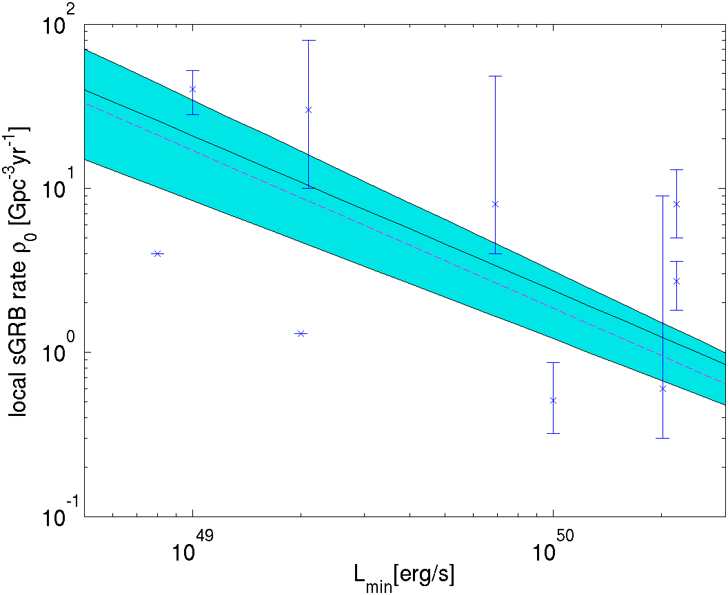
Figure 8: The local sGRB rate as a function of the minimal luminosity for SFR1 (black solid line) and SFR2 (magenta dashed line) for the best-fit parameters in the log-normal time delay model. The shaded area is the joint $1\sigma$ uncertainty range of the local sGRB rate for both SFR1 and SFR2 based models. The error bars represent the results of previous studies - see table 4 for details.

	local rate ($\rho_{0}$)	$L_{min}$	This work
	[Gpc-3yr-1]	[erg/s]	for a similar $L_{min}$
Ando (2004) (1)	$0.51^{+0.36}_{-0.19}$	$10^{50}$	$2.1_{-0.9}^{+1.0}$
Guetta & Piran (2006) (1)	$0.6^{+8.4}_{-0.3}$	$2\times 10^{50}$	$1.1_{-0.4}^{+0.4}$
Guetta & Piran (2006) (2)	$8^{+40}_{-4}$	$7\times 10^{49}$	$3.0_{-1.4}^{+1.6}$
Guetta & Piran (2006) (1)	$30^{+50}_{-20}$	$2\times 10^{49}$	$9.4_{-4.9}^{+6.6}$
Nakar et al. (2006)	$40^{+12}_{-12}$	$10^{49}$	$18.9_{-10.5}^{+15.5}$
Guetta & Stella (2009) (1)	$1.3$	$2\times 10^{49}$	$9.8_{-5.1}^{+6.9}$
Guetta & Stella (2009) (3)	$4$	$0.8\times 10^{49}$	$23.4_{-13.2}^{+20.0}$
Dietz (2011)	$1.05^{+0.5}_{-0.9}$	$4\times 10^{50}(*)$	$0.5_{-0.2}^{+0.2}$
Coward et al. (2012)	$8^{+5}_{-3}$	$2\times 10^{50}(*)$	$1.0_{-0.4}^{+0.4}$
Siellez et al. (2013)	$2.7^{+0.9}_{-0.9}$	$2\times 10^{50}(*)$	$1.0_{-0.4}^{+0.4}$
This work	$4.1_{-1.9}^{+2.3}$	$5\times 10^{49}$	$4.1_{-1.9}^{+2.3}$

Table 4: A comparison of different estimates of the local short bursts rate, without a beaming correction.
Notes: (*) When no luminosity low-end cutoff (erg/s) is specified we take the cutoff to be just below the least luminous burst in the given sample. (1) For a model with time delay $1/t$ for $t>20Myr$ with respect to Porciani & Madau (2001) SF2. (2) For a model with a constant rate at all redshifts. (3) For a constant time delay of 6 Gyr with respect to Porciani & Madau (2001) SF2.

A comparison with other works considering the time delay with respect to the SFR cannot be done directly since other papers use different SFR models. Many older papers use the Porciani & Madau (2001) SF2 model which has been disfavored by later observations. There is however an agreement that sGRBs do not follow the SFR directly i.e. without delay. Ando (2004), Guetta & Piran (2006), Guetta & Stella (2009), favor a rate model which is delayed with respect to Porciani & Madau (2001) SF2. Hao & Yuan (2013) adopt an hierarchical structure formation model from Pereira & Miranda (2010), in which the SFR is derived using a Press-Schechter like formalism. That SFR peaks at $z\approx 3$ and then drop very slowly as the redshift increases (by a factor $\sim 4$ form $z=3$ to $z=10$), more resembling the Porciani & Madau (2001) SF2 SFR rather than the SFRs we consider here. Consistently with our results, they found that the power-law time delay model is disfavored and that the log-normal time delay distribution with $\tau\gtrsim 3$ Gyr is consistent with the data.

In the frame-work of ns² or a nsbh mergers, the narrow time delay distribution implies an extremely narrow distribution of the initial separation between the two compact objects. This time delay is less sensitive to the other parameters, like masses or eccentricities and the allowed spread in the time delay is consistent with the expected variation in these parameters. For canonical 1.4 solar masses neutron stars and circular orbits the initial separation are (Shapiro & Teukolsky, 1983) $2.0\times 10^{11}$ cm and $2.2\times 10^{11}$ cm for $2.9$ Gyr and $3.9$ Gyr respectively (the best time delay values for SFR1 and SFR2 respectively). These values vary very little at the allowed range of time delays. For example for $t_{d}=2.9^{\pm 0.4}$ Gyr the resulting range is $r_{0}=2.04^{\pm 0.08}\times 10^{11}$ cm. These initial separations are smaller than the main-sequence radii of main sequence progenitors of the neutron-stars which are typically $>3\times 10^{11}$ cm. This implies that the binaries have undergone a common envelope phase. This narrow range of initial separations seems to suggest that this common envelope phase ends with a very narrow range of separations and that somehow the formation of the second neutron star, by a supernova explosion of or via another mechanism (Piran & Shaviv, 2005) does not disrupt this significantly.

It is important to recall that the last conclusion that follows from the result concerning the narrow distribution of time delays depends critically on the lack of non-Collapsar sGRBs at $z>1.2$, a distant at which Swift becomes insensitive to the lower end of the sGRB luminosity distribution. A somewhat wider time delay distribute would have arisen if $z>1.2$ non-Collapsar sGRBs would have been observed by Swift. It is possible that such bursts have been detected but their redshift was not measured and hence they were not included in the sample. This would have changed significantly the conclusion concerning the narrow range of initial separation.

As ns² mergers (or bhns mergers), which are the most likely sources of sGRBs, are the prime targets of GW detectors we turn to discuss the implications of our results to GW detection. The approximate detection horizon of ns² merger by Advanced LIGO/Virgo and other planned advanced GW detectors is $300$ Mpc. As the estimated local rate depends on the lower limit for the luminosity taken we must refer to a minimum luminosity value when predicting detection rates. With our “canonical” estimate of the lowest peak luminosity $5\times 10^{49}$ erg/s we expect within this radius $0.06\pm 0.03yr^{-1}$ sGRBs detected by Swift and $0.4\pm 0.2yr^{-1}$ detected by Fermi/GBM. (see table 5 for the rates for two other lower limits on peak luminosity: the lowest observed peak luminosity by Swift , $2.2\times 10^{50}$ erg/s, and an optimistic lower limit of $10^{49}$ erg/s.). These values reflect probabilities for simultaneous detection of a sGRB with a GW signal (Kochanek & Piran, 1993). The estimated GW detection horizon for a bhns merger is $\sim 1$ Gpc. The expected joint detection rate is $0.7\pm 0.3yr^{-1}$ and $5\pm 2yr^{-1}$ for Swift and Fermi respectively for the canonical lowest peak luminosity $5\times 10^{49}$ erg/s (see table 5).

When considering the overall detection rate of the GW detectors one has to consider the fact that sGRBs are most likely beamed. Using a typical beaming factor of $f_{b}^{-1}\approx 30$ (see also Fong et al., 2012) and the “canonical” lower limit on the peak luminosity of $5\times 10^{49}$  erg/s the event rate within a radius of $300Mpc$ becomes $14_{-7}^{+8}yr^{-1}$ and the corresponding rate of detection of bhns mergers with a GW detection horizon of 1 Gpc is $5.1_{-2.4}^{+3.0}\times 10^{2}$ (see table 5 for other values of the lowest peak luminosity).

horizon	$L_{min}$	GW det. alone	Fermi	Swift
$[Gpc]$	$[$erg/s $]$	$yr^{-1}$	$yr^{-1}$	$yr^{-1}$
0.3	$10^{49}$	$64_{-36}^{+53}$	$1.0_{-0.5}^{+0.7}$	$0.14_{-0.07}^{+0.11}$
	$5\times 10^{49}$	$14_{-7}^{+8}$	$0.4\pm 0.2$	$0.06\pm 0.03$
	$2.2\times 10^{50}$	$3.7\pm 1.4$	$0.11\pm 0.04$	$0.02\pm 0.01$
1	$10^{49}$	$2.4_{-1.3}^{+1.9}\times 10^{3}$	$6_{-3}^{+4}$	$0.8_{-0.4}^{+0.6}$
	$5\times 10^{49}$	$5.1_{-2.4}^{+3.0}\times 10^{2}$	$5\pm 2$	$0.7\pm 0.3$
	$2.2\times 10^{50}$	$138\pm 53$	$5_{-2}^{+1}$	$0.5_{-0.2}^{+0.1}$

Table 5: The expected GW detection rates with Advanced LIGO/Virgo for ns² mergers (detection horizon $\sim$ 0.3 Gpc) or bhns mergers (detection horizon $\sim$ 1 Gpc), for different lower limits on the peak luminosity $L_{min}$. Also given are the rates of a coincident detection of the GW and a detection of a sGRB by Fermi or by Swift.

Finally it is interesting to consider the implications of these findings to the possibility that sGRBs are the sources of heavy r-process material Lattimer & Schramm (1974); Eichler et al. (1989); Freiburghaus et al. (1999). This possibility received recently a lot of attention in view of the possible detection of a IR signal 6 days (in the source rest frame) after the short GRB 130603B (Tanvir et al., 2013; Berger et al., 2013). If the interpretation of this IR signal as macronova is correct it implies that $0.02-0.04$ r-process material were produced in this event (Barnes & Kasen, 2013; Hotokezaka et al., 2013; Grossman et al., 2014; Piran et al., 2014). As there are about $10^{4}m_{\odot}$ of heavy ($A\>110$) r-process material in the Milky Way, a few$\times~{}10^{5}$ such merger events are required to produce this material. Integration of the sGRB rate and using an effective density of $0.01$ Mpc^-3 Milky Way like galaxies we obtain that there were $\approx 1.4\times 10^{4}$ mergers beamed towards us within the Milky Way. If all mergers produces a similar amount of r-process material than a modest beaming factor of $f_{b}^{-1}\approx 20-30$ suffices to explain the observed abundance of these elements. A critical consideration when proposing ns² mergers as sources of heavy r-process material is the observations of such elements in some very low metallicity ($\log_{10}[Fe/H]\approx 3$) stars (Woolf et al., 1995; Shetrone, 1996; Burris et al., 2000; Cayrel et al., 2001; Hill et al., 2002). The $Eu/Fe$ ratio varies strongly at this low metallicity, which agrees with the possibility that the heavy r-process elements are produced in rare events, but the question arises are there mergers so early on. A constant time delay of $\sim 2$ Gyr is incompatible with such early merger events. However, the best fit power law time delay model (which was the less favored one in our analysis) yields $1000(f_{b}^{-1}/30)$ mergers before redshift 5 and $10^{4}(f_{b}^{-1}/30)$ mergers before redshift 3, and those might be sufficient to produce the required amounts of heavy r-process material sufficiently early on.

Acknowledgments

The research was supported by an ERC advanced grant (GRBs) and by the I-CORE Program of the Planning and Budgeting Committee and The Israel Science Foundation (grant No 1829/12).

References

- Ando (2004) Ando S., 2004, J. Cosmology Astropart. Phys, 6, 7
- Band et al. (1993) Band D. et al., 1993, ApJ, 413, 281
- Barnes & Kasen (2013) Barnes J., Kasen D., 2013, ApJ, 775, 18
- Barthelmy et al. (2005) Barthelmy S. D. et al., 2005, Space Sci. Rev., 120, 143
- Belczynski et al. (2002) Belczynski K., Kalogera V., Bulik T., 2002, ApJ, 572, 407
- Berger (2005) Berger E., 2005, GRB Coordinates Network, 3801, 1
- Berger (2006a) Berger E., 2006a, GRB Coordinates Network, 5952, 1
- Berger (2006b) Berger E., 2006b, GRB Coordinates Network, 5965, 1
- Berger (2007) Berger E., 2007, GRB Coordinates Network, 5995, 1
- Berger (2014) Berger E., 2014, ARA&A, 52, 43
- Berger et al. (2013) Berger E., Fong W., Chornock R., 2013, ApJ, 774, L23
- Berger et al. (2007) Berger E., Morrell N., Roth M., 2007, GRB Coordinates Network, 7154, 1
- Berger & Soderberg (2005) Berger E., Soderberg A. M., 2005, GRB Coordinates Network, 4384, 1
- Bloom et al. (2006) Bloom J. S. et al., 2006, GRB Coordinates Network, 5238, 1
- Bouwens et al. (2011) Bouwens R. J. et al., 2011, Nature, 469, 504
- Bouwens et al. (2012) Bouwens R. J. et al., 2012, ApJ, 752, L5
- Bromberg et al. (2013) Bromberg O., Nakar E., Piran T., Sari R., 2013, ApJ, 764, 179
- Burris et al. (2000) Burris D. L. et al., 2000, ApJ, 544, 302
- Cayrel et al. (2001) Cayrel R. et al., eds, Astrophysical Ages and Times Scales Vol. 245 of Astronomical Society of the Pacific Conference Series, First Measurement of the Uranium/Thorium Ratio in a Very Old Star: Implications for the Age of the Galaxy. p. 244
- Cenko et al. (2010) Cenko S. B. et al., 2010, GRB Coordinates Network, 10389, 1
- Chornock & Berger (2011) Chornock R., Berger E., 2011, GRB Coordinates Network, 11518, 1
- Chornock et al. (2013) Chornock R., Lunnan R., Berger E., 2013, GRB Coordinates Network, 15307, 1
- Cohen & Piran (1995) Cohen E., Piran T., 1995, ApJ, 444, L25
- Covino et al. (2007) Covino S. et al., 2007, GRB Coordinates Network, 6666, 1
- Coward et al. (2013) Coward D. M. et al., 2013, MNRAS, 432, 2141
- Coward et al. (2012) Coward D. M. et al., 2012, MNRAS, 425, 2668
- Cucchiara et al. (2006) Cucchiara A., Cannizzo J., Berger E., 2006, GRB Coordinates Network, 5924, 1
- Cucchiara et al. (2007) Cucchiara A. et al., 2007, GRB Coordinates Network, 6665, 1
- Cucchiara et al. (2013) Cucchiara A., Perley D., Cenko S. B., 2013, GRB Coordinates Network, 14748, 1
- Cucciati et al. (2012) Cucciati O. et al., 2012, A&A, 539, A31
- D’Avanzo et al. (2007) D’Avanzo P. et al.., 2007, GRB Coordinates Network, 7152, 1
- D’Elia et al. (2013) D’Elia V. et al., 2013, GRB Coordinates Network, 15310, 1
- Dezalay et al. (1996) Dezalay J. P. et al., 1996, ApJ, 471, L27
- Dietz (2011) Dietz A., 2011, A&A, 529, A97
- Eichler et al. (1989) Eichler D., Livio M., Piran T., Schramm D. N., 1989, Nature, 340, 126
- Foley et al. (2005) Foley R. J., Bloom J. S., Chen H.-W., 2005, GRB Coordinates Network, 3808, 1
- Foley et al. (2013) Foley R. J. et al., 2013, GRB Coordinates Network, 14745, 1
- Fong et al. (2012) Fong W. et al., 2012, ApJ, 756, 189
- Fong et al. (2011) Fong W. et al., 2011, ApJ, 730, 26
- Fong et al. (2013) Fong W. et al., 2013, ApJ, 769, 56
- Freiburghaus et al. (1999) Freiburghaus C., Rosswog S., Thielemann F.-K., 1999, ApJ, 525, L121
- Gehrels et al. (2004) Gehrels N. et al., 2004, ApJ, 611, 1005
- Gehrels et al. (2005) Gehrels N. et al., 2005, Nature, 437, 851
- Grossman et al. (2014) Grossman D., Korobkin O., Rosswog S., Piran T., 2014, MNRAS, 439, 757
- Guetta & Piran (2005) Guetta D., Piran T., 2005, A&A, 435, 421
- Guetta & Piran (2006) Guetta D., Piran T., 2006, A&A, 453, 823
- Guetta & Stella (2009) Guetta D., Stella L., 2009, A&A, 498, 329
- Hao & Yuan (2013) Hao J.-M., Yuan Y.-F., 2013, A&A, 558, A22
- Hill et al. (2002) Hill V. et al., 2002, A&A, 387, 560
- Hopkins & Beacom (2006) Hopkins A. M., Beacom J. F., 2006, ApJ, 651, 142
- Hotokezaka et al. (2013) Hotokezaka K. et al., 2013, Phys. Rev. D, 87, 024001
- Kochanek & Piran (1993) Kochanek C. S., Piran T., 1993, ApJ, 417, L17
- Kouveliotou et al. (1996) Kouveliotou C. et al., eds, American Institute of Physics Conference Series Vol. 384 of American Institute of Physics Conference Series, Correlations between duration, hardness and intensity in GRBs. pp 42–46
- Kouveliotou et al. (1993) Kouveliotou C. et al., 1993, ApJ, 413, L101
- Lattimer & Schramm (1974) Lattimer J. M., Schramm D. N., 1974, ApJ, (Letters), 192, L145
- Lattimer & Schramm (1974) Lattimer J. M., Schramm D. N., 1974, ApJ, 192, L145
- Levesque et al. (2009) Levesque E. et al., 2009, GRB Coordinates Network, 9264, 1
- Lien et al. (2014) Lien A. et al., 2014, ApJ, 783, 24
- Nakar (2007) Nakar E., 2007, Phys. Rep., 442, 166
- Nakar et al. (2006) Nakar E., Gal-Yam A., Fox D. B., 2006, ApJ, 650, 281
- Nava et al. (2011) Nava L. et al., 2011, A&A, 530, A21
- Oesch et al. (2013) Oesch P. A. et al., 2013, ApJ, 773, 75
- Paciesas et al. (2012a) Paciesas W. S. et al., 2012a, ApJS, 199, 18
- Paciesas et al. (2012b) Paciesas W. S. et al., 2012b, VizieR Online Data Catalog, 219, 90018
- Pereira & Miranda (2010) Pereira E. S., Miranda O. D., 2010, MNRAS, 401, 1924
- Perley et al. (2008) Perley D. A. et al., 2008, GRB Coordinates Network, 7889, 1
- Perley et al. (2007) Perley D. A. et al., 2007, GRB Coordinates Network, 7140, 1
- Piran (1992a) Piran T., 1992a, ApJ, 389, L45
- Piran (1992b) Piran T., 1992b, ApJ, 389, L45
- Piran et al. (2014) Piran T., Korobkin O., Rosswog S., 2014, ArXiv e-prints
- Piran & Shaviv (2005) Piran T., Shaviv N. J., 2005, Physical Review Letters, 94, 051102
- Planck Collaboration et al. (2013) Planck Collaboration Ade P. A. R. et al., 2013, ArXiv e-prints
- Porciani & Madau (2001) Porciani C., Madau P., 2001, ApJ, 548, 522
- Prochaska et al. (2005) Prochaska J. X. et al., 2005, GRB Coordinates Network, 3700, 1
- Rau et al. (2009) Rau A., McBreen S., Kruehler T., 2009, GRB Coordinates Network, 9353, 1
- Rowlinson et al. (2010) Rowlinson A. et al., 2010, MNRAS, 408, 383
- Sakamoto et al. (2008) Sakamoto T. et al., 2008, ApJS, 175, 179
- Sakamoto et al. (2011) Sakamoto T. et al., 2011, ApJS, 195, 2
- Sanchez-Ramirez et al. (2013) Sanchez-Ramirez R. et al., 2013, GRB Coordinates Network, 14747, 1
- Shapiro & Teukolsky (1983) Shapiro S. L., Teukolsky S. A., 1983, Black holes, white dwarfs, and neutron stars: The physics of compact objects
- Shetrone (1996) Shetrone M. D., 1996, AJ, 112, 1517
- Siellez et al. (2013) Siellez K., Boer M., Gendre B., 2013
- Soderberg et al. (2006) Soderberg A. M. et al., 2006, ApJ, 650, 261
- Tanvir et al. (2013) Tanvir N. R. et al., 2013, Nature, 500, 547
- Thoene et al. (2010) Thoene C. C. et al., 2010, GRB Coordinates Network, 10971, 1
- Thoene et al. (2009) Thoene C. C. et al., 2009, GRB Coordinates Network, 9269, 1
- Thone et al. (2013) Thone C. C. et al., 2013, GRB Coordinates Network, 14744, 1
- Wanderman & Piran (2010) Wanderman D., Piran T., 2010, MNRAS, 406, 1944
- Woolf et al. (1995) Woolf V. M., Tomkin J., Lambert D. L., 1995, ApJ, 453, 660
- Xu et al. (2013) Xu D. et al., 2013, GRB Coordinates Network, 14757, 1