Node Classification in Uncertain Graphs

Abstract

In many real applications that use and analyze networked data, the links in the network graph may be erroneous, or derived from probabilistic techniques. In such cases, the node classification problem can be challenging, since the unreliability of the links may affect the final results of the classification process. If the information about link reliability is not used explicitly, the classification accuracy in the underlying network may be affected adversely. In this paper, we focus on situations that require the analysis of the uncertainty that is present in the graph structure. We study the novel problem of node classification in uncertain graphs, by treating uncertainty as a first-class citizen. We propose two techniques based on a Bayes model and automatic parameter selection, and show that the incorporation of uncertainty in the classification process as a first-class citizen is beneficial. We experimentally evaluate the proposed approach using different real data sets, and study the behavior of the algorithms under different conditions. The results demonstrate the effectiveness and efficiency of our approach.

1 Introduction

The problem of collective classification is a widely studied one in the context of graph mining and social networking applications. In this problem, we have a network containing nodes and edges, which can be represented as a graph. Nodes in this network may be labeled, but it is not necessary that all nodes have a label. Typically, such labels may represent some properties of interest in the underlying network. This is a setting that appears in several situations in practice.

Some examples of such labeled networks in real scenarios are listed below:

• In a bibliographic network, nodes correspond to authors, and the edges between them correspond to co-authorship links. The labels in the bibliographic network may correspond to subject areas that experts are interested in. It is desirable to use this information in order to classify other nodes in the network.

• In a biological network, the nodes correspond to the proteins. The edges may represent the possibility that the proteins may interact. The labels may correspond to properties of proteins [4].

• In a movie-actor network, the nodes correspond to the actors. The edges correspond to the co-actor relationship between the different actors. The labels correspond to the pre-dominant genre of the movie of the actor.

• In a patent network, the nodes correspond to patent assignees. The edges model the citations between the respective patents. The labels correspond to the class categories.

In such networks, only a small fraction of the nodes may be labeled, and these labels may be used in order to determine the labels of other nodes in the network. This problem is popularly referred to as collective classification or label propagation [17, 19, 20, 32, 25, 39, 40, 41], and a wide variety of methods have been proposed for this problem.

The problem of data uncertainty has been widely studied in the database literature [18, 2, 3], and also presents numerous challenges in the context of network data [44]. In many real networks, the links are uncertain in nature, and are derived with the use of a probabilistic process. In such cases, a probability value may be associated with each edge. Some examples are as follows:

• In biological networks, the links are derived from probabilistic processes. In such cases, the edges have uncertainty associated with them. Nevertheless, such probabilistic networks are valuable, since the probability information on the links provides important information for the mining process.

• The links in many military networks are constantly changing and may be uncertain in nature. In such cases, the analysis needs to be performed with imperfect knowledge about the network.

• Networks in which some links have large failure probabilities are uncertain in nature.

• Many human interaction networks can be created from real interaction processes, and such links are often uncertain in networks.

Thus, such networks can be represented as probabilistic networks, in which we have probabilities associated with the existence of links. Such probabilities can be very useful for improving the effectiveness of problems such as collective classification. Furthermore, these networks may also have properties associated with nodes, that are denoted by labels.

Recent years have seen the emergence of numerous methods for uncertain graph management [24, 27, 36] and mining [27, 29, 26, 31, 35, 42, 43], in which uncertainty is used directly as a first-class citizen. However, none of these methods address the problem of collective graph classification.

One possibility is to use sampling of possible worlds on the edges in order to generate different instantiations of the underlying network. The collective classification problem can be solved on these different instantiations, and voting can be used in order to report the final class label. The major disadvantage with this approach is that the sampling process could result in a sparse or disconnected network which is not suited to the collective classification problem. In such cases, good class labels cannot be easily produced with a modest number of samples.

In this paper, we investigate the problem of collective classification in uncertain networks with a more direct use of the uncertainty information in the network . We design two algorithms for collective classification. The first algorithm uses a probabilistic approach, which explicitly accounts for the uncertainty in the links in the classification.

The second algorithm works with the assumption that most of the information in the network is encoded in high-probability links, and low-probability links sometimes even degrade the quality. Therefore, the algorithm uses the links with high probability in earlier iterations, and successively relaxes the constraints on the quality of the underlying links. The idea is that a greater caution in early phases of the algorithm ensures convergence to a better optimum.

The contributions we make in this paper can be summarized as follows.

• We introduce the problem of collective classification in uncertain graphs, where uncertainty is associated with the edges of the graph, and provide a formal definition for this problem.

• We introduce two algorithms based on iterative probabilistic labeling that incorporate the uncertainty of edges in their operation. These algorithms are based on a Bayes formulation, which enables them to capture correlations across different classes, leading to improved accuracy.

• We perform an extensive experimental evaluation, using two real datasets from diverse domains. We evaluate our techniques using a multitude of different conditions, and input data characteristics. The results demonstrate the effectiveness of the proposed techniques and serve as guidelines for the practitioners in the field.

This paper is organized as follows. In Section 2 we survey prior studies on collective classification and on mining uncertain networks. In Section 3, we formally define the problem of collective classification in uncertain networks. In Section 4, we present our model and two algorithms for collective classification. We discuss the space and time complexity of our proposal in Section 5, and we present the results of our experimental evaluation in Section 6. Finally, we discuss the conclusions in Section 7.

2 Related Work

The problem of node classification has been studied in the graph mining literature, and especially relational data in the context of label or belief propagation [37, 39, 40]. Such propagation techniques are also used as a tool for semi-supervised learning with both labeled and unlabeled examples [41]. Collective classification [33, 32, 19] refers to semi-supervised learning methods that exploit the network structure and node class labels to improve the classification accuracy. These techniques are mostly based on the assumption of homophily in social networks [21, 34]: neighboring nodes tend to belong to the same class. A technique has been proposed in [32], which uses link-based similarity for node-classification in directed graphs. Recently, collective classification methods have also been used in the context of blogs [19]. In [20], Bilgic et al. discuss the problem of overcoming the propagation of erroneous labels by asking the user for more labels. A method for performing collective classification of email speech acts has been proposed by Carvalho et al. in [22], exploiting the sequential correlation of emails. In [25], Ji et al. integrate the classification of nodes in heterogeneous networks with ranking. Methods for leveraging label consistency for collective classification have been proposed in [39, 40, 41].

Recently, the database and data mining community has investigated the problem of uncertain data mining widely [18, 14].

A comprehensive review of the proposed models and algorithms can be found in [8]. Several database systems supporting uncertain data have been proposed, such as Conquer [9], Trio [10], MistiQ [7], MayMBS [11] and Orion [12].

The "possible worlds" model, introduced by Abiteboul et al. [13], formalizes uncertainty by defining the space of the possible instantiations of the database. Instantiations must be consistent with the semantics of the data. For example, in a graph database representing moving object trajectories there may be be different configurations of the edges where each node represents a region in the space. However, an edge cannot connect a pair of nodes that represent a pair of non-neighboring regions. The main advantage of the "possible worlds" model is that the formulations of the queries originally designed to cope with certain data can be directly applied on each possible instantiation. Many different alternatives have then been propose to aggregate the results across the different instantiations.

Despite its attractiveness, the number of possible worlds explodes very quickly and even their enumeration becomes intractable problem. To overcome these issues, simplifying assumptions have been introduced to leverage its simplicity: The tuple- and the attribute-uncertainty models [16, 8]. In the attribute-uncertainty model, the uncertain tuple is represented by means of multiple samples drawn from its Probability Density Function (PDF). In contrast, in the tuple-uncertainty model the value of the tuple is fixed but the tuple itself may not exist.

Similar simplifications have been considered for graph databases where nodes may or may not exist (node-uncertainty) and edges are associated with an existence probability (edge-uncertainty). The underlying uncertainty model can then be used to generate graph instances, eventually considering additional generation rules to consider correlations across different nodes and edges. In this study we combine a Bayes approach and the edge-uncertainty model.

The problem of uncertain graph mining has also been investigated extensively. The most common problems studied in uncertain graph management are those of nearest neighbor query processing [24, 36], reachability computation [28] and subgraph search [38]. In the context of uncertain graph mining, the problems commonly studied are frequent subgraph mining [35, 42, 43], reliable subgraph mining [27], and clustering [26, 31]. Recently, the problem of graph classification has also been studied for the uncertain scenario [29], though these methods are designed for classification of many small graphs, in which labels are attached to the entire graph rather than a node in the graph. Typical social and web-based scenarios use a different model of collective classification, in which the labels are attached to nodes in a single large graph.

In this work, we study the problem of collective classification in the context of uncertain networks, where the underlying links are uncertain. Uncertainty impacts negatively on the classification accuracy. First, links may connect sub-networks of very different density, causing the propagation of erroneous labels. Second, the farthest distance between two nodes tends to be smaller in very noisy networks, because of the presence of a larger number of uncertain edges, which include both true and spurious edges. This reduces the effectiveness of iterative models because of the faster propagation of errors. Some of our techniques, which drop uncertain links at earlier stages of the algorithm, are designed to ameliorate these effects.

3 Collective Classification Problem

In this section, we formalize the problem of collective classification after introducing some definitions. An uncertain network is composed of nodes whose connections may exist with some probability.

Definition 3.1 (Uncertain Network)

An uncertain network is denoted by $G=(N,A,P)$, with node set $N$, edge set $A$ and probability set $P$. Each edge $(i,j)\in A$ is associated with a probability value $p_{ij}\in P$. This is the probability that edge $(i,j)$ exists in the network.

We assume that the network is undirected, though the method can easily be extended to the directed scenario. We can assume that the $|N|\times|N|$ matrix $P$ has entries which are denoted by $p_{ij}$ and $p_{ij}=p_{ji}$. A node $i\in N$ can be associated with a label, representing its membership in a class. For ease in notation, we assume that node labels are integers.

Definition 3.2 (Node Label)

Given a set of labels $S$ drawn from a set of integers $\{1\ldots l\}$, we denote the label of node $i$ by $L(i)$. If a node $i$ is unlabeled, the special label $0$ is used.

We can now introduce the definition of the collective classification problem on uncertain graphs.

Problem 3.1 (Uncertain Collective Classification)

Given an uncertain network $G=(N,A,P)$ and the subset of labeled nodes $T_{0}=\{i\in N:L(i)\neq 0\}$, predict the labels of nodes in $N-T_{0}$.

Figure 1 shows an example of an uncertain network. Nodes $1$, $2$, and $3$ are labeled white, and nodes $5$, $7$, and $8$ are labeled black. The label of nodes $4$ and $6$ is unknown. The aim of collective classification is to assign labels to nodes $4$ and $6$.

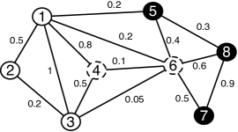
Figure 1: Example of uncertain network. Nodes $\{1,2,3\}$ are labeled white and nodes $\{5,8,7\}$ are labeled black, while labels for nodes $\{4,6\}$ are unknown. Edges between nodes exist with some probability.

4 Iterative Probabilistic Labeling

In this section, we first present the algorithm for iterative probabilistic labeling. A Bayes approach is used in order to perform the iterative probabilistic labeling. This method models the probabilities of the nodes belonging to different classes on the basis of the adjacency behavior of the nodes. The Bayes approach can directly incorporate the edge uncertainty probabilities into the estimation process. We continue with a second algorithm that builds upon the first one, and is based on iterative edge augmentation. Finally, we describe a variation of the second algorithm that is a linear combination of two classifiers.

4.1 Bayes Approach

The overall approach for the labeling process uses a Bayesian model for the labeling. In the rest of the paper, we refer to this algorithm as uBayes. Given that we have an unlabeled node $r$, which is adjacent to $s$ other nodes denoted by $t_{1}\ldots t_{s}$, how do we determine the label of the node $r$? It should be noted that the concept of adjacency is also uncertain, because the edges are associated with probabilities of existence. This is particularly true, when the edge probabilities are relatively small, since the individual network instantiations are likely to be much sparser and different than the probabilistic descriptions. Furthermore, for each edge $(i,j)$ we need to estimate the probability of the node $j$ having a particular label value, given the current value of the label at node $i$. This is done with the use of training data containing the labels and edges in the network. These labels and edges can be used to construct a Bayesian model of how the labels on the nodes and edges relate to one another.

The algorithm uses an iterative approach, which successively labels more nodes in different iterations. This is the set $T$ of nodes whose labels will not be changed any further by the algorithm. Initially, the algorithm starts off by setting $T$ to the initial set of (already) labeled nodes $T_{0}$. The set in $T$ is expanded to $T\cup T^{+}$ in each iteration, where $T^{+}$ is the set of nodes not yet labeled that are adjacent to the labeled nodes in $T$. If $T^{+}$ is empty, either all nodes have been labeled or there is a disconnected component of the network whose nodes are not in $T_{0}$.

The expanded set of labeled nodes are added to the set of training nodes in order to compute the propagation probabilities on other edges. Thus, the overall algorithm iteratively performs the following steps:

• Estimating the Bayesian probabilities of propagation from the current set of edges.

• Computing the probabilities of the labels of the nodes in $N-T$.

• Expanding the set of the nodes in $T$, by adding the set of nodes from $T^{+}$, whose labels have the highest probability for a particular class.

These steps are repeated until no more nodes reachable from the set $T$ remain to be labeled. We then label all the remaining nodes in a single step, and terminate. The overall procedure for performing the analysis is illustrated in Algorithm 1. It now remains to discuss how the individual steps in Algorithm 1 are performed.

Algorithm uBayes(Graph: $G$
Uncertainty Prob.: $P$, Initial Labeling: $T_{0}$ );
begin
	$T=T_{0}$;
	while (not termination) do
	begin
		Compute edge propagation probabilities;
		Compute node label probabilities in $N-T$;
		Expand $T$ with $T^{+}$ nodes;
	end
end

Algorithm 1 Broad Framework for Uncertain Classification.

The two most important steps are the computation of the edge-propagation probabilities and the expansion of the node labels with the use of the Bayes approach. For a given edge $(i,j)$ we estimate $P(L(i)=p|L(j)=q)$. This is estimated from the data in each iteration by examining the labels of nodes which have already been decided. Therefore, the training process is successively refined in each iteration. Therefore, the value of $P(L(i)=p|L(j)=q)$ can be estimated by examining those edges for which one end point contains a label of $q$. Among these edges, we compute the fraction for which the other end point contains a label of $p$. For example, in the network shown in Figure 1 the probability $P(L(6)=black|L(5)=black)$ is estimated as $(0.3+0.9)/(0.3+0.9+0.2)=0.85$. The label of node $6$ is unknown, and it is not considered in the calculation. Note that this is simply equal to the probability that both end points of an edge are black, if one of them is black. Therefore, one can compute the uncertainty weighted conditional probabilities for this in the training process of each iteration.

This provides an estimate for the conditional probability. We note that in some cases, the number of nodes with a label of either $p$ or $q$ may be too small for a robust estimation. The following smoothing techniques are useful in reducing the effect of ill-conditioned probabilities:

• We always add a small value $\delta$ to each probability. This is similar to Laplacian smoothing and prevents any probability value from being zero, which would cause problems in a multiplicative Bayes model.

• In some cases, the estimation may not be possible when labels do not exist for either nodes $p$ or $q$. In those cases, we set the probabilities to their prior values.

The prior is defined as the value of $P(L(i)=p)$, and is equal to the fraction of currently labeled nodes with label of $p$. The prior therefore defines the default behavior in cases where the adjacency information cannot be reasonably used in order to obtain a better posteriori estimation.

For an unlabeled node $r$, whose neighbors $i_{1}\ldots i_{s}$ have labels $t_{1}\ldots t_{s}$, we estimate its (unnormalized) probability by using the naive Bayes rule over all the adjacent labeled neighbors. This is therefore computed as follows:

$$P(L(r)=p|L(i_{1})=t_{1}\ldots L(i_{s})=t_{s})\propto\ \ \ \ \ \ \ \ \ \ \ \ \ \ \$$

$$\ \ \ \ \ \ \ \ \ \ \ \ P(L(r)=p)\cdot\prod_{k}P(L(i_{k})=t_{k}|L(r)=p)$$

Note that the above model incorporates the uncertainty probabilities directly within the product term of the equation. We can perform the estimation for each of the different classes separately. If desired, one can normalize the probability values to sum to one. However, such a normalization is not necessary in our case, since the only purpose of the computation is to determine the highest probability value in order to assign labels.

4.2 Iterative Edge Augmentation

The approach mentioned above is not very effective when a large fraction of the edges are noisy. In particular, if many edges have a low probability, this can have a significant impact on the classification process.

Figure 2 shows an example. Nodes $1$, $2$, are labeled white, and nodes $3$, $4$, $6$, $7$, $8$ and $9$ are labeled black. The label of node $5$ is unknown and must be assigned by the algorithm. We observe that ignoring the edges whose existence probability is lower than $0.5$ is beneficial for the correct classification of node $5$.

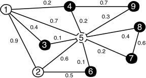
Figure 2: Example of uncertain network. Nodes $1$, $2$, are labeled white, and nodes $3$, $4$, $6$, $7$, $8$ and $9$ are labeled black, while the label of node $5$ is unknown and must be assigned by the algorithm. Edges between nodes exist with some probability.

Therefore, we use an iterative augmentation process in order to reduce the impact of such edges, by instead favoring the positive impact of high quality edges in the collective classification process. The idea is to activate only a subset of the edges for use on the modeling process. In other words, edges which are not activated are not used in the modeling. We call this algorithm uBayes+.

We adopt a model inspired by automatic parameter selection in machine learning. Note that, analogous to parameter selection, the choice of a particular subset of high quality links, corresponds to a configuration of the network, and we would like to determine an optimal configuration for our approach. In order to do this, we split the set of labeled nodes $T_{0}$ into two subsets: a training set denoted by $T_{train}$ and a hold out set denoted by $T_{hold}$. The ratio of the $T_{0}$ nodes that are assigned to the training set $T_{train}$ is denoted by $\beta$, a user-defined parameter.

The purpose of the hold out set is to aid optimal configuration selection by checking the precise value of the parameters at which the training model provides optimal accuracy over the set of nodes in $T_{hold}$. We use labels of nodes in $T_{train}$ for the learning process, while using labels of nodes in $T_{hold}$ as for the evaluation of accuracy at a particular configuration of the network. (Note that a label is never used for both the training and the hold out set, in order to avoid overfitting.) The idea is to pick the ratio of active edges in such a way so as to optimize the accuracy on the hold out set. This ensures that an optimal fraction of the high quality edges are used for the labeling process.

We start off considering a small fraction of the high probability edges, iteratively expanding the subset of active edges by enabling some of the inactive edges with the highest probabilities. The ratio of active edges is denoted by the parameter $\theta$. Ideally, we want to activate only the edges that contribute positively to the classification of unlabeled nodes. Given a configuration of active edges, we measure their goodness as the estimated accuracy on labels of nodes in $T_{hold}$. The value of $\theta$ that leads to the highest accuracy, denoted by $\theta^{*}$, is used as the ratio of edges with the highest probability to activate on the uncertain network $G$. The resulting network is then used as input for the iterative probabilistic labeling algorithm (uBayes).

Despite optimizing accuracy by selecting the best ratio of edges to be considered, the basic model described above is not very efficient, because it requires multiple evaluations of the iterative probabilistic labeling algorithm. In particular, it requires us to vary the parameter $\theta$ and evaluate accuracy, in order to determine $\theta^{*}$.

A more efficient technique for identifying $\theta^{*}$ can be obtained by evaluating the accuracy for different values of $\theta$ on a sample of the uncertain network $G$ (rather than the full network) as follows. We generate a new uncertain network $G^{\prime}=(N^{\prime},A^{\prime},P^{\prime})$ by sampling $\alpha\cdot|N|$ nodes from $G$ uniformly at random, and retaining the edges from $A$ and probabilities from $P$ referring to these sampled nodes. $\alpha$ is a user-defined parameter that controls the ratio of nodes sampled from $G$ and it implies the size of the sampled uncertain network $G^{\prime}$. The initial set of labeled nodes in the sampled uncertain network $G^{\prime}$ is $T_{0}^{\prime}=T_{0}\cap N^{\prime}$. We split the set of nodes in $T_{0}^{\prime}$ into two random subsets, $T_{train}^{\prime}$ and $T_{hold}^{\prime}$, respectively. The number of nodes in $T_{train}^{\prime}$ is $\beta\cdot|T_{0}^{\prime}|$. We start off considering $\theta|A^{\prime}|$ edges with the highest probabilities, expanding iteratively the subset of active edges at each iteration by increasing $\theta$. The goodness of parameter $\theta$ is estimated as the accuracy of node labels in $T_{hold}^{\prime}$. Let $\theta^{*}$ be the value of $\theta$ leading to the highest accuracy. We activate $\theta^{*}|N|$ edges with highest probability in $G$. The resulting network is then used as input for the iterative probabilistic labeling (Algorithm 1). The overall algorithm is illustrated in Algorithm 2.

Algorithm uBayes+(Graph: $G$
Uncertainty Prob.: $P$, Initial Labeling: $T_{0}$,
Sampled nodes ratio: $\alpha$, Train nodes ratio: $\beta$);
begin
	$N^{\prime}$ = Random sample of $\alpha\cdot|N|$ nodes from $N$;
	$A^{\prime}$ = Edges $(i,j)$ in $A$ with $i,j\in N^{\prime}$;
	$(T_{hold}^{\prime},T_{train}^{\prime})=split(T_{0}\cap N^{\prime},\beta)$;
	$F=\theta\cdot|A^{\prime}|$ edges in $A^{\prime}$ with
	greatest existence probability;
	while ($F\neq A^{\prime}$) do
	begin
		Construct graph $G^{F}=(N^{\prime},F)$;
		$uBayes(G^{F},P,T_{train})$;
		Test accuracy using nodes in $T_{hold}$;
		Expand edges in $F$ with top edges in $A^{\prime}$;
	end
		Construct graph $G^{*}=(N,F)$ with best
		configuration (corresponding to $\theta^{*}$);
		$uBayes(G^{*},P,T_{0})$;
end

Algorithm 2 Iterative Edge Augmentation for Uncertain Classification

We note that the frequencies used to estimate conditional and prior probabilities across the different configurations in Algorithm 2 can be efficiently maintained in an incremental fashion.

4.3 Combining different classifiers

In this section we propose a third algorithm, uBayes+RN. It uses an ensemble methodology in order to further improve robustness in scenarios, where some deterministic classifiers can provide good results over some subsets of nodes, but not over all the nodes. uBayes+RN is the linear combination of two classifiers: the uBayes+ algorithm and the Relational Neighbor (RN) classifier [33]. The RN classifier is defined as follows:

$$P_{RN}(L(r)=p)=\frac{1}{Z}\sum_{k:L(i_{k})=p}p_{i_{k}r}$$ (1)

where $p_{i_{k}r}$ is the probability and $Z=\sum_{k}p_{i_{k}r}$. The uBayes+ and RN algorithms are combined as follows:

$$P(L(r)=p)=$$

$$P(L(r)=p|L(i_{1})=t_{1}\ldots L(i_{s})=t_{s})\cdot\delta P_{RN}(L(r)=p)$$

where $\delta$ controls the influence of the RN classifier during the collective classification process. When $\delta=0$ then uBayes+RN degenerates to uBayes+, while when $\delta=1$ the two classifiers are weighted equally. Note that this is a simple linear combination. We used this combination, since it sometimes provides greater robustness in the classification process.

5 Complexity analysis

In this section, we discuss the complexity of the proposed algorithms.

We start with uBayes, which for the computation of the initial statistics requires $O(|N|+|A|)$ (label priors and conditional label probabilities). Assuming that the cardinality of the set of immediate unlabeled neighbors of nodes in $T$ (remember that $T$ represents the set of currently labeled nodes) is at most $N_{max}$, and that the number of neighbors for a particular node is at most $A_{max}$, each iteration can be decomposed as follows. The computation of new unlabeled nodes requires $O(N_{max}A_{max})$. The computation of edge propagation probabilities requires $O(N_{max}A_{max})$. The computation of node label probabilities requires $O(N_{max}A_{max})$. Summing up, each iteration requires $O(N_{max}A_{max})$. Assuming that all unlabeled nodes will be labeled in $K$ iterations, the algorithm cost is $O(K|N||A|)$, where $K<<|N|$. Space complexity is $O(|N||A|)$.

For algorithm uBayes+, the computation of the uncertain network sample $G^{\prime}=(N^{\prime},A^{\prime},P^{\prime})$ requires $O(|N|+|A|)$. Active edges are maintained using a priority list, whose initialization requires $O(|A|)$. Each iteration of the iterative automatic parameter selection procedure can be decomposed as follows. Algorithm 1 (used by uBayes+) requires $O(|N^{\prime}||A^{\prime}|)$. Testing the classification accuracy requires $O(|N^{\prime}|)$. Expanding the set of active edges requires $O(|A^{\prime}|log(|A^{\prime}|))$. Summing up, each iteration requires:

$$O(log(|A^{\prime}|)|N^{\prime}||A^{\prime}|).$$ (2)

Finally, the last call to Algorithm 1 requires $O(K|N||A|)$. Assuming that the parameter selection procedure terminates after $K^{\prime}$ iterations, the algorithm cost is $O(|N|+|A|+K^{\prime}(log(|A^{\prime}|)|N^{\prime}||A^{\prime}|))$. Simplifying, the cost is $O(log(|A|)|N||A|)$. The space complexity is $O(|N||A|)$.

Note that algorithms uBayes+RN and uBayes+ have the same space and time complexity.

6 Experimental Results

In this section, we evaluate the proposed techniques under different settings, in terms of both accuracy and performance.

We implemented all techniques in C++ using the Standard Template Library (STL) and Boost libraries, and ran the experiments on a Linux machine equipped with an Intel Xeon 2.40GHz processor and 16GB of RAM.

The reported times do not include the initial loading time, which was constant over all methods. The results were obtained from $5$ independent runs. For all experiments we report the averages and $95\%$ confidence intervals.

6.1 Data Sets

In our experiments, we used two data sets for which edge probabilities can be estimated, as described below.

DBLP: The DBLP data set [30] is the most comprehensive citation network of curated records of scientific publications in computer science. In our experiments, we consider the subset of publications from $1980$ to $2010$. The data set consists of $922,673$ nodes and $3,389,272$ edges. Nodes represent authors and edges represent co-authorship relations. The edge probability is an estimate of the probability that two authors co-authored a paper in a year selected randomly during their period of activity. For example, if a pair of authors published papers in ten different years and they both published papers for twenty years, then their edge probability is $0.5$. (We consider the union of their periods of activity.) We used 14 class labels, that represent different research fields in computer science. The corresponding labels and their frequencies are illustrated in Table 1. The labels were generated by using a set of top conferences and journals in these areas, and the most frequent label in the author’s publications is used as the author’s label. In our data set, $16\%$ of the nodes are labeled. The rest were not labeled, because the corresponding authors did not have publications in the relevant conferences and journals.

Id	Name	Prior probability
$C_{1}$	Verification & Testing	$0.06758$
$C_{2}$	Computer Graphics	$0.01974$
$C_{3}$	Computer Vision	$0.04144$
$C_{4}$	Networking	$0.1301$
$C_{5}$	Data Mining	$0.09498$
$C_{6}$	Operating systems	$0.06058$
$C_{7}$	Computer Human Interaction	$0.05361$
$C_{8}$	Software Engineering	$0.01935$
$C_{9}$	Machine Learning	$0.1543$
$C_{10}$	Bioinformatics	$0.1936$
$C_{11}$	Computing Theory	$0.04008$
$C_{12}$	Information Security	$0.05364$
$C_{13}$	Information Retrieval	$0.044$
$C_{14}$	Computational Linguistics	$0.02711$

Table 1: Node labels and label priors of the DBLP dataset.

Id	Name	Prior probability
$C_{1}$	Verification & Testing	$0.06758$
$C_{2}$	Computer Graphics	$0.01974$
$C_{3}$	Computer Vision	$0.04144$
$C_{4}$	Networking	$0.1301$
$C_{5}$	Data Mining	$0.09498$
$C_{6}$	Operating systems	$0.06058$
$C_{7}$	Computer Human Interaction	$0.05361$
$C_{8}$	Software Engineering	$0.01935$
$C_{9}$	Machine Learning	$0.1543$
$C_{10}$	Bioinformatics	$0.1936$
$C_{11}$	Computing Theory	$0.04008$
$C_{12}$	Information Security	$0.05364$
$C_{13}$	Information Retrieval	$0.044$
$C_{14}$	Computational Linguistics	$0.02711$

Table 2: Class labels and corresponding conference keywords

US Patent Data Set: The US Patent data set [23] is a citation network of US utility patents. In our experiments, we consider patents issued from $1970$ to $1990$. The network contained $108,658$ nodes and $1,059,822$ edges. A node represents a patent assignee and there is an edge between two assignees if there is at least a patent from one assignee citing a patent from the other assignee. The edge probability is an estimate of the probability that one of the two assignee cites the other assignee. For example, assignee $A$ cites $20$ patents of which $5$ are assigned to assignee $B$, then their edge probability is $0.25$. A category is assigned to each patent. The most frequent category in the assignee’s patents is used as assignee label. Table 3 reports the label class names and their frequencies. These labels cover $66\%$ of nodes. We used class label as ground truth. Although the raw input data sets are curated manually, class labels are derived algorithmically and may be noisy. For example, if an assignee holds only two patents belonging to different categories, we pick one of these two categories randomly as the assignee label. In other words, we do not model our confidence in the derived class labels. Results show that the proposed algorithms is robust to this lack of information.

Id	Name	Prior probability
$C_{1}$	Chemical	$0.2077$
$C_{2}$	Computers & communications	$0.07945$
$C_{3}$	Drugs & Medical	$0.0859$
$C_{4}$	Electrical & Electronic	$0.19292$
$C_{5}$	Mechanical	$0.434$

Table 3: Node labels and label priors of the Patent data set.

6.2 Perturbation

We also used perturbed data sets to stress-test the methods. The advantage of such data is the ability to test the effectiveness with varying uncertainty level, and other sensitivity parameters. This provides a better idea of the inherent variations of the performance. Perturbed data sets are generated by either adding noisy edges or by removing existing edges to and from the real data sets. Noisy edges are new edges with low probability. The edge probability is sampled from a normal distribution $N(0,\sigma)$ in the interval $(0,1]$. The parameter $\sigma$ controls the probability standard deviation. As it gets larger the average edge probability increases, eventually interfering with edges in the real data sets. The parameter $\phi$ controls the ratio of noisy edges. Given the edge set $A$ of a real data set, the number of added noisy edges is $\phi\cdot|A|$.

The existing edges to be removed are selected by sampling the edge set $A$ uniformly at random. Existing edges are removed after adding noisy edges. The parameter $\Phi$ controls the ratio of edges to be removed. Given the edge set $A$ of a perturbed data set, the number of retained edges is $(1-\Phi)|A|$. The selection criterion is also known as probability sampling.

The existing labeled nodes to be unlabeled are selected by sampling the node set $N$ randomly. The parameter $\Gamma$ controls the ratio of labeled nodes, whose label is to be removed. Given the node set $N$ of a real data set, the number of labeled nodes whose label is removed is $(1-\Gamma)|N|$.

Unless otherwise specified, we used the following default perturbation parameters. The ratio of noisy edges ($\phi$) is $3$ and the standard deviation of noisy edges ($\sigma$) is $0.25$. By default, we do not remove any edges or labels. Thus, $\Phi$ equals zero, and the ratio of known labels for the data sets are those reported in Section 6.1.

6.3 Evaluation Methodology

The accuracy is assessed by using repeated random sub-sampling validation. We randomly partition the nodes into training and validation subsets which are denoted by $N_{T}$ and $N_{V}$ respectively. We use $2/3$ of the labeled nodes for training, and the remaining $1/3$ for validation. Even if $2/3$ may appear as a large fraction, note that it refers to the labeled nodes in the ground truth (that is rather limited).

For each method, we compute the confusion matrix $M$ on the $N_{V}$ set, where $M_{ij}$ is the count of nodes labeled as $i$ in the ground-truth that are labeled as $j$. Accuracy is defined as the ratio of true positives for all class labels:

$$Accuracy=\frac{1}{|N_{V}|}\sum M_{ii}$$ (3)

If all nodes are labeled correctly, $M$ is a diagonal matrix. The experiment is repeated several times to get statistically significant results.

In all experiments we use the following parameters for the uBayes+ algorithm. The ratio nodes of the sampled uncertain network ($\alpha$) is $0.2$. Among the sampled nodes, the ratio nodes used for training ($\beta$) is $0.1$. In order to identify $\theta^{*}$, the algorithm varies $\theta$ between $0.05$ and $1$ in $20$ steps. These values were determined experimentally, and are the same for both datasets (the performance of the algorithms remains stable for small variations of these parameters).

We compared our techniques to two algorithms, which are the wvRN [33] and Sampling methods. Since these algorithms trade accuracy for running time, we limited the running time of these two algorithms to the time spent by the uBayes method. The wvRN method estimates the probability of node $i$ to have label $j$ as the weighted sum of class membership probabilities of neighboring nodes for label $j$. Thus, it works with a weighted deterministic representation of the network, where the edge probabilities are used as weights. Relaxation labeling is then used for inference. We additionally consider a version of the wvRN algorithm, wvRN-20, that is not time-bounded, but is bound to terminate after $20$ iterations in the label relaxation procedure. As we discuss later, the accuracy of wvRN converges quickly and does not improve further after $20$ iterations for both data sets.

The sampling algorithm samples networks in order to create deterministic representations. For each sampled instantiation, the RN algorithm [33] is used. Note that links in sampled instantiations either exist or do not exist, and link weights are set to $1$. This algorithm estimates class membership probabilities by voting on the different labelings over different instantiations of the network. The class with the largest vote is reported as the relevant label.

6.4 Classification Quality Results

In this section, we report our results on accuracy under a variety of settings using both real and perturbed data sets. The first experiment shows the accuracy by varying the ratio of noisy edges ($\phi$) for the algorithms uBayes, uBayes+, wvRN, wvRN-20 and Sampling. The results for the DBLP and Patent data sets are reported in Figures 5(a) and 5(b), respectively. The Sampling algorithm is the worst performer on both data sets, followed by wvRN and wvRN-20. On the DBLP data set, the accuracy of wvRN-20 is slightly higher than that of wvRN. The uBayes and uBayes+ algorithms are the best performers, with uBayes+ achieving higher accuracy on the DBLP dataset when the ratio of noisy edges is above $200\%$. We observe that there is nearly no difference among the uBayes, uBayes+, wvRN and wvRN-20 algorithms on both datasets when $\phi=0$, while the percentage improvement in accuracy from wvRN-20 to uBayes+ when $\phi=5$ ($500\%$) is up to $49\%$ for DBLP and $7\%$ for Patent. It is worth noting that, as the ratio of noisy edges increases, the accuracy for Sampling increases in the Patent data set. This is due to the high probability of label $C_{5}$ ($0.434$), as reported in Table 3, which eventually dominates the process.

In the next experiment, we varied the standard deviation of the probability of the noisy edges ($\sigma$) for algorithms uBayes, uBayes+, wvRN, wvRN-20 and Sampling. The results for the DBLP and the Patent data sets are reported in Figures 5(a) and 5(b), respectively. The Sampling algorithm again does not perform well, followed by the wvRN and wvRN-20 algorithms. The uBayes+ algorithm is consistently the best performer on the DBLP dataset, while there is nearly no difference between the uBayes+ and uBayes algorithms on the Patent data set. The higher accuracy of uBayes and uBayes+ is explained by their ability to better capture correlations between different class labels, a useful feature when processing noisy data sets. The better performance of uBayes+ is due to its ability to ignore noisy labels that contribute negatively to the overall classification process. uBayes+ is more accurate than wvRN-20 with a percentage improvement up to $83\%$ in the DBLP data set and $10\%$ in the Patent data set, which represents a significant advantage.

In the following experiment, we evaluate the accuracy when varying the ratio of labeled nodes ($\Gamma$) for algorithms uBayes, uBayes+, wvRN, wvRN-20 and Sampling. (Default perturbation parameters are considered for the retained edges.) The results for the DBLP and Patent data sets are reported in Figures 5(a) and 5(b) respectively. In the DBLP dataset, the wvRN algorithm performs better than wvRN-20, while there is virtually no difference on the Patent dataset. The uBayes+ algorithm is consistently the best performer on the DBLP dataset, while it performs slightly worse than uBayes on the Patent data set when $\Gamma$ is below $0.2$ ($20\%$). We observe that the percentage improvement of uBayes+ over wvRN-20 is $50\%$ on the DBLP dataset and $11\%$ on the Patent dataset. The Sampling algorithm exhibits the lowest accuracy.

(a) DBLP

(b) Patent

Figure 3: Accuracy with varying ratio of noisy edges for algorithms uBayes, uBayes+, wvRN, wvRN-20 and Sampling.

(a) DBLP

(b) Patent

Figure 4: Accuracy with varying standard deviation of probability of noisy edges for uBayes, uBayes+, wvRN, wvRN-20 and Sampling algorithms.

(a) DBLP

(b) Patent

Figure 5: Accuracy with varying ratio of labeled nodes for uBayes, uBayes+, wvRN, wvRN-20 and Sampling algorithms.

We now stress-test the proposed techniques by randomly removing a percentage of edges ($\Phi$), as detailed in Section 6.2. The results for the DBLP and the Patent data sets are reported in Figures 8(a) and 8(b), respectively. Sampling consistently performs at the lower range, followed by wvRN and wvRN-20. uBayes and uBayes+ perform consistently better on the DBLP dataset, with uBayes+ performing poorly when the ratio of retained edges is below $60\%$. In this case, the resulting network is less connected, and the uncertain network sample used for the automatic parameter tuning becomes less robust to noisy conditions. In the DBLP dataset, the percentage improvement of uBayes+ over wvRN-20 is up to $49\%$.

(a) DBLP

(b) Patent

Figure 6: Accuracy with varying ratio of retained edges for uBayes, uBayes+, wvRN, wvRN-20 and Sampling algorithms.

(a) DBLP

(b) Patent

Figure 7: Time performance with varying ratio of noisy edges for uBayes, uBayes+ and wvRN-20 algorithms.

(a) DBLP

(b) Patent

Figure 8: Time performance with varying standard deviation of probability of noisy edges for Bayes, Bayes+ and wvRN-20 algorithms.

In Table 4, we report the confusion matrices for the DBLP and Patent data sets for the uBayes+ algorithm. The confusion matrix provides some interesting insights, especially for cases where nodes were misclassified. Cell $i,j$ reports the number of nodes with ground truth label $C_{i}$ classified with label $j$. We observe that $C_{4}$, $C_{9}$ and $C_{10}$ labels (networking, machine-learning and bioinformatics) in the DBLP data set lead to many misclassifications. This can be explained by the fact that these are the most frequent labels in the network (refer to Table 1), and therefore have a higher probability of being selected. We also observe that misclassifications convey interesting and useful information. For example, excluding the $C_{4}$, $C_{9}$ and $C_{10}$ classes, most of the misclassifications for class “Data Mining" are due to the “Information Retrieval" class, and vice versa. This points to the fact that the two communities are related to each other. Similar observations can be made on the Patent data set. For example, the “Chemical" and “Drugs & Medical" classes overlap, and show corresponding behavior in the confusion matrices.

	$C_{1}$	$C_{2}$	$C_{3}$	$C_{4}$	$C_{5}$	$C_{6}$	$C_{7}$	$C_{8}$	$C_{9}$	$C_{10}$	$C_{11}$	$C_{12}$	$C_{13}$	$C_{14}$
$C_{1}$	$\mathbf{1943}$	$7$	$9$	$116$	$19$	$58$	$11$	$38$	$364$	$595$	$32$	$35$	$4$	$7$
$C_{2}$	$3$	$\mathbf{620}$	$30$	$21$	$12$	$7$	$37$	$3$	$125$	$131$	$6$	$4$	$3$	$1$
$C_{3}$	$15$	$49$	$\mathbf{1088}$	$51$	$25$	$18$	$13$	$3$	$489$	$261$	$11$	$8$	$11$	$3$
$C_{4}$	$55$	$21$	$22$	$\mathbf{3907}$	$70$	$161$	$38$	$19$	$915$	$1076$	$69$	$87$	$23$	$8$
$C_{5}$	$12$	$17$	$26$	$182$	$\mathbf{2237}$	$92$	$49$	$45$	$960$	$791$	$60$	$79$	$126$	$37$
$C_{6}$	$60$	$26$	$12$	$311$	$86$	$\mathbf{1482}$	$26$	$39$	$423$	$464$	$105$	$80$	$35$	$7$
$C_{7}$	$7$	$36$	$13$	$43$	$14$	$12$	$\mathbf{1396}$	$20$	$463$	$584$	$4$	$15$	$39$	$15$
$C_{8}$	$7$	$3$	$0$	$18$	$10$	$15$	$18$	$\mathbf{619}$	$113$	$128$	$4$	$8$	$7$	$4$
$C_{9}$	$37$	$46$	$271$	$279$	$152$	$47$	$72$	$23$	$\mathbf{5422}$	$1287$	$74$	$85$	$110$	$104$
$C_{10}$	$42$	$32$	$81$	$274$	$127$	$80$	$45$	$26$	$692$	$\mathbf{8410}$	$79$	$58$	$44$	$45$
$C_{11}$	$28$	$10$	$7$	$135$	$22$	$168$	$9$	$13$	$258$	$321$	$\mathbf{950}$	$46$	$5$	$3$
$C_{12}$	$27$	$13$	$18$	$236$	$62$	$70$	$33$	$26$	$428$	$483$	$35$	$\mathbf{1230}$	$20$	$7$
$C_{13}$	$7$	$9$	$14$	$73$	$94$	$22$	$67$	$29$	$452$	$415$	$15$	$18$	$\mathbf{873}$	$82$
$C_{14}$	$5$	$5$	$5$	$40$	$20$	$8$	$14$	$2$	$268$	$226$	$12$	$11$	$34$	$\mathbf{756}$

Table 4: Confusion matrix for DBLP dataset. True positives are indicated in bold.

	$C_{1}$	$C_{2}$	$C_{3}$	$C_{4}$	$C_{5}$
$C_{1}$	$\mathbf{939}$	$5$	$34$	$79$	$3861$
$C_{2}$	$21$	$\mathbf{328}$	$4$	$98$	$1421$
$C_{3}$	$181$	$0$	$\mathbf{279}$	$26$	$1567$
$C_{4}$	$96$	$108$	$26$	$\mathbf{574}$	$3798$
$C_{5}$	$292$	$63$	$26$	$133$	$\mathbf{10020}$

Table 5: Confusion matrix for Patent data set. True positives are indicated in bold.

Finally, we report the accuracy of the uBayes+RN algorithm when varying the parameter $\delta$ between $0$ and $1$. Recall that $\delta$ controls the influence of the RN classifier on the overall classification process. In our experiments with both data sets, the accuracy of uBayes+RN was always slightly better than uBayes+, but never more than $5\%$. We observed nearly no difference among the different $\delta$ configurations. In the interest of space, we omit the detailed results.

We next provide some real examples of labeling results obtained with uBayes+ on the Patent dataset. The “Atari Inc." and “Sega Enterprises, Ltd" companies, which belong to the hall of fame of the video game industry, were not assigned to any category. Our algorithm correctly classified them as “Computers & Communications". Similarly, the companies “North American Biologicals, Inc" and “Bio-Chem Valve, Inc" were correctly labeled as “Drugs & Medical", since they are both involved in drug development and pharmaceutical research. Interestingly, “Starbucks Corporation" was labeled as “Chemical". Taking a close look at their patents, it turns out that a large fraction of them describe techniques for enhancing flavors and aromas that involve chemical procedures. Evidently, having labels for all the nodes in the graph allows for improved query answering and data analysis in general.

6.5 Efficiency Results

In this section, we assess running time efficiency on a variety of settings using both real and perturbed data sets. Figures 8(a) and 8(b) show the CPU time required by the algorithms when varying the ratio of noisy edges, for the DBLP and Patent data sets, respectively. Note that Sampling has the same time performance as uBayes. The uBayes+ algorithm is nearly three times slower than uBayes. This is due to the automatic parameter tuning approach employed by the uBayes+ algorithm We observe that the performance of wvRN-20 almost always considerably worse than both uBayes and uBayes+. The same observation is true when we vary the standard deviation of the probability of the noisy edges (see Figures 8(a) and 8(b)). Note that the inference in the wvRN algorithm is based on labeling relaxation, whose complexity is proportional to the size of the network and remains constant across iterations. On the contrary, the iterative labeling that uBayes and uBayes+ use for their inference model becomes faster with each successive iteration, since it needs to visit a smaller part of the network. As the results show, the standard deviation does not affect the time performance of the algorithms. These experiments demonstrate that the two proposed algorithms effectively combine low running times with high accuracy and robustness levels.

In the final set of experiments, we evaluated the accuracy of all algorithms as a function of the time required for algorithmic execution by the baselines. Since the baselines tradeoff between running time and accuracy, it is natural to include the running time in the comparison process. In this case, we removed the constraint that wvRN and Sampling end their processing after a fixed amount of time or a specific number of iterations, and examined how their accuracy changes when the number of iterations (and consequently, processing time) increases. For reference, we also include the uBayes and uBayes+ algorithms, which execute in a fixed amount of time. The results for the DBLP and Patent data sets are depicted in Figures 9 and 10 respectively. The graphs show that the accuracy of wvRN and Sampling is slightly increasing with time, but reaches an almost stable state after the first $10$ iterations. (In our experiments, we stopped wvRN after $28$ iterations in the DBLP data set and $16$ iterations in the Patent data set, and the Sampling algorithm after $92$ iterations in the DBLP data set and $28$ iterations in the Patent dataset). Nevertheless, the uBayes and uBayes+ algorithms achieve significantly better results in a much lower running time.

Figure 9: Accuracy with varying execution times for uBayes, uBayes+, wvRN and Sampling algorithms for the DBLP data set.

Figure 10: Accuracy with varying execution times for uBayes, uBayes+, wvRN and Sampling algorithms for the Patent data set.

7 Conclusions

Uncertain graphs are becoming increasingly popular in a wide variety of data domains. This is due to the statistical methods used to infer many networks, such as protein interaction networks and other link-prediction based methods. Consequently, the problem of collective classification has become particularly relevant for determining node properties in such networks.

In this paper, we formulate the collective classification problem for uncertain graphs, and describe effective and efficient solutions for this problem. To this effect, we describe an iterative probabilistic labeling method, based on the Bayes model, that treats uncertainty on the edges of the graph as first class citizens. In the proposed approach, the uncertainty probabilities of the links are used directly in the labeling process. Furthermore, the methodology we describe allows for automatic parameter selection.

We have performed an experimental evaluation of the proposed approach using diverse, real-world datasets. The results show significant advantages of using such an approach for the classification process over more conventional methods, which do not directly use uncertainty probabilities.

Acknowledgments
Part of this work was supported by the FP7 EU IP project KAP (grant agreement no. 260111). Work of the second author was sponsored by the Army Research Laboratory under cooperative agreement number W911NF-09-2-0053.

References

- [1] M. Dallachiesa, C. C. Aggarwal, and T. Palpanas. Node Classification in Uncertain Graphs SSDBM, 2014, to appear.
- [2] M. Dallachiesa, I. F. Ilyas, and T. Palpanas. Top-k Nearest Neighbor Search In Uncertain Data Series PVLDB, 2015, to appear.
- [3] M. Dallachiesa, B. Nushi, K. Mirylenka, and T. Palpanas. Uncertain time-series similarity: Return to the basics. PVLDB, 2012.
- [4] L. Eronen and H. Toivonen. Biomine: predicting links between biological entities using network models of heterogeneous databases. BMC bioinformatics, 13(1):119, 2012.
- [5] P. Boldi, F. Bonchi, A. Gionis, and T. Tassa. Injecting uncertainty in graphs for identity obfuscation. Proceedings of the VLDB Endowment, 5(11):1376–1387, 2012.
- [6] Y. Yuan, G. Wang, L. Chen, and H. Wang. Efficient keyword search on uncertain graph data. Knowledge and Data Engineering, IEEE Transactions on, 25(12):2767–2779, 2013.
- [7] N. N. Dalvi and D. Suciu. Efficient query evaluation on probabilistic databases. In International Conference on Very Large Data Bases (VLDB), pages 864–875, 2004.
- [8] C. C. Aggarwal and P. S. Yu. A survey of uncertain data algorithms and applications. IEEE Transactions on Knowledge and Data Engineering (TKDE), 21(5):609–623, 2009.
- [9] A. Fuxman, E. Fazli, and R. J. Miller. Conquer: Efficient management of inconsistent databases. In Proceedings of the 2005 ACM SIGMOD International Conference on Management of Data, pages 155–166. ACM, 2005.
- [10] P. Agrawal, O. Benjelloun, A. D. Sarma, C. Hayworth, S. U. Nabar, T. Sugihara, and J. Widom. Trio: A system for data, uncertainty, and lineage. In International Conference on Very Large Data Bases (VLDB), pages 1151–1154, 2006.
- [11] L. Antova, C. Koch, and D. Olteanu. Query language support for incomplete information in the maybms system. In International Conference on Very Large Data Bases (VLDB), pages 1422–1425, 2007.
- [12] S. Singh, C. Mayfield, S. Mittal, S. Prabhakar, S. E. Hambrusch, and R. Shah. Orion 2.0: native support for uncertain data. In ACM SIGMOD International Conference on Management of Data, pages 1239–1242, 2008.
- [13] S. Abiteboul, P. C. Kanellakis, and G. Grahne. On the representation and querying of sets of possible worlds. In ACM SIGMOD International Conference on Management of Data, pages 34–48, 1987.
- [14] N. N. Dalvi and D. Suciu. Management of probabilistic data: foundations and challenges. In ACM Symposium on Principles of Database Systems (PODS), pages 1–12, 2007.
- [15] Y. Gao. Shortest path problem with uncertain arc lengths. Computers & Mathematics with Applications, 62(6):2591–2600, 2011.
- [16] J. Jestes, G. Cormode, F. Li, and K. Yi. Semantics of ranking queries for probabilistic data. IEEE Transactions on Knowledge and Data Engineering (TKDE), 23(12):1903–1917, 2011.
- [17] C. Aggarwal, H. Wang. Managing and Mining Graph Data, Springer, 2010.
- [18] C. Aggarwal. Managing and Mining Uncertain Data, Springer, 2009.
- [19] S. Bhagat, G. Cormode, I. Rozenbaum. Applying link-based classification to label blogs, WebKDD/SNA-KDD, 2007.
- [20] M. Bilgic, L. Getoor. Effective label acquisition for collective classification, ACM SIGKDD Conference on Knowledge Discovery and Data Mining (KDD), 2008.
- [21] P. Blau. Inequality and heterogeneity: A primitive theory of social structure. Free Press, NY, 1977.
- [22] V. de Carvalho, W. Cohen, On the collective classification of email “speech acts", ACM Special Interest Group on Information Retrieval (SIGIR), 2005.
- [23] B. Hall, A. Jaffe, M. Trajtenberg. The NBER patent citation data file: Lessons, insights and methodological tools, National Bureau of Economic Research, 2001.
- [24] M. Hua, J. Pei. Probabilistic path queries in road networks: traffic uncertainty aware path selection. International Conference on Extending Database Technology (EDBT), 2010.
- [25] M. Ji, J. Han, M. Danilevsky. Ranking-based classification of heterogeneous information networks. ACM SIGKDD Conference on Knowledge Discovery and Data Mining (KDD), 2011.
- [26] G. Kollios, M. Potamias, E. Terzi. Clustering large probabilistic graphs. IEEE Transactions on Knowledge and Data Engineering (TKDE), 99, 2011.
- [27] R. Jin, L. Liu, C. Aggarwal. Discovering Highly Reliable Subgraphs in Uncertain Graphs, ACM SIGKDD Conference on Knowledge Discovery and Data Mining (KDD), 2011.
- [28] R. Jin, L. Liu, B. Ding, H. Wang. Distance-constraint reachability computation in uncertain graphs. International Conference on Very Large Data Bases (VLDB), 2011.
- [29] X. Kong, P. Yu, X. Wang, A. Ragin. Discriminative Feature Selection for Uncertain Graph Classification. SIAM International Conference on Data Mining (SDM), 2013.
- [30] M. Ley, S. Dagstuhl. DBLP Dataset, http://dblp.uni-trier.de/xml/ August, 2012
- [31] L. Liu, R. Jin, C. Aggrawal, Y. Shen. Reliable Clustering on Uncertain Graphs, IEEE International Conference on Data Mining series (ICDM), 2012.
- [32] Q. Lu, L. Getoor, Link-based classification, International Conference on Machine Learning (ICML), 2003.
- [33] S. Macskassy, F. Provost. A simple relational classifier. Technical report, 2003.
- [34] M. McPherson, L. Smith-Lovin, J. Cook. Birds of a feather: Homophily in social networks. Annual review of sociology, pages 415–444, 2001.
- [35] O. Papapetrou, E. Ioannou, D. Skoutas. Efficient discovery of frequent subgraph patterns in uncertain graph databases. International Conference on Extending Database Technology (EDBT), 2011.
- [36] M. Potamias, F. Bonchi, A. Gionis, G. Kollios. -nearest neighbors in uncertain graphs. Proceedings of the Very Large Data Base Endowment (PVLDB), 2010.
- [37] B. Taskar, P. Abbeel, D. Koller, Discriminative probabilistic models for relational data, UAI, 2002.
- [38] Y. Yuan, G. Wang, H. Wang, L. Chen. Efficient subgraph search over large uncertain graphs. International Conference on Very Large Data Bases, 2011.
- [39] D. Zhou, O. Bousquet, T. N. Lal, J. Weston, B. Schölkopf, Learning with local and global consistency, Neural Information Processing Systems (NIPS), 2004.
- [40] D. Zhou, J. Huang, B. Schölkopf, Learning from labeled and unlabeled data on a directed graph, International Conference on Machine Learning (ICML), 2005.
- [41] X. Zhu, Z. Ghahramani, J. Lafferty, Semi-supervised learning using gaussian fields and harmonic functions, ICML, 2003.
- [42] Z. Zou, H. Gao, J. Li. Discovering frequent subgraphs over uncertain graph databases under probabilistic semantics. ACM SIGKDD Conference on Knowledge Discovery and Data Mining (KDD), 2010.
- [43] Z. Zou, J. Li, H. Gao, S. Zhang. Finding top-k maximal cliques in an uncertain graph. International Conference on Data Engineering (ICDE), 2010.
- [44] J. Ren, S. D. Lee, X. Chen, B. Kao, R. Cheng, and D. Cheung. Naive bayes classification of uncertain data. In Data Mining, 2009. ICDM’09. Ninth IEEE International Conference on, pages 944–949. IEEE, 2009.
- [45] J. Dahlin and P. Svenson. A method for community detection in uncertain networks. In Intelligence and Security Informatics Conference (EISIC), 2011 European, pages 155–162. IEEE, 2011.