Random mixtures of polycyclic aromatic hydrocarbon spectra match interstellar infrared emission

The mid-infrared (IR; 5-15 $\mu$m) spectrum of a wide variety of astronomical objects exhibits a set of broad emission features at 6.2, 7.7, 8.6, 11.3 and 12.7 $\mu$m. About 30 years ago it was proposed that these signatures are due to emission from a family of UV heated nanometer-sized carbonaceous molecules known as polycyclic aromatic hydrocarbons (PAHs), causing them to be referred to as aromatic IR bands (AIBs). Today, the acceptance of the PAH model is far from settled, as the identification of a single PAH in space has not yet been successful and physically relevant theoretical models involving “true” PAH cross sections do not reproduce the AIBs in detail. In this paper, we use the NASA Ames PAH IR Spectroscopic Database, which contains over 500 quantum-computed spectra, in conjunction with a simple emission model, to show that the spectrum produced by any random mixture of at least 30 PAHs converges to the same ’kernel’-spectrum. This kernel-spectrum captures the essence of the PAH emission spectrum and is highly correlated with observations of AIBs, strongly supporting PAHs as their source. Also, the fact that a large number of molecules are required implies that spectroscopic signatures of the individual PAHs contributing to the AIBs spanning the visible, near-infrared, and far infrared spectral regions are weak, explaining why they have not yet been detected. An improved effort, joining laboratory, theoretical, and observational studies of the PAH emission process, will support the use of PAH features as a probe of physical and chemical conditions in the nearby and distant Universe.

1 Introduction

The mid-infrared spectrum (IR; 5-15 $\mu$m) of astronomical objects is dominated by band emission strongest at 6.2, 7.7, 8.6, 11.3 and 12.7 $\mu$m and were referred to as the unidentified IR (UIR) bands. Discovered during the 1970’s, this family of emission features are now generally attributed to mixtures of polycyclic aromatic hydrocarbons; large, chicken-wire shaped molecules of fused aromatic rings, and closely related species (e.g., Draine & Li 2007; Tielens 2008; Siebenmorgen et al. 2014, and references therein). In space, free floating PAH molecules become highly vibrationally excited upon the absorption of a single photon (ultraviolet – near-infrared; Mattioda et al. 2005; Draine & Li 2007). Relaxation occurs through emission of IR photons at characteristic wavelengths, leaving the tell-tale spectroscopic fingerprints of aromatic molecules. The features that comprise this apparently universal spectral signature dominates the mid-IR spectrum of many bright astronomical objects and contain a wealth of information about the physical conditions in the emitting regions (e.g., Joblin & Tielens 2011, and references therein). However PAHs are no silent witnesses, they are active participants and drive many aspects of the galactic evolution from cold collapsing clouds to stellar death (see Tielens (2008)).

Initially, the AIB spectrum observed in the ISM of dusty galaxies seemed invariant, yet as observations improved variations in relative band strengths and subtle shifts in peak positions and profiles were reported. In particular, an evolution of the ratio of the short (i.e., at 6.2, 7.7 and 8.6 $\mu$m) to long wavelength bands (i.e., at 11.2 and 12.7 $\mu$m) was identified, both in the galactic (Bregman et al. 1989; Joblin et al. 1996) and extragalactic (Galliano et al. 2008) ISM. These variations have been attributed to a varying degree of PAH ionization (Szczepanski & Vala 1993; Hudgins & Allamandola 1995a, b).

However, the acceptance of the PAH model is far from settled. Recently, the PAH hypothesis was contested by Kwok & Zhang (2011) who propose that this emission arises from complex organic solids with disorganized structures. These claims were quickly rebutted (Li & Draine 2012). Nonetheless, the lack of the identification of a single PAH molecule in space remains troublesome for some.

In this Letter, we show how the astronomical AIB spectrum can be reproduced from first principles using the quantum-chemically calculated PAH spectra from the NASA Ames PAH IR Spectroscopic Database (www.astrochem.org/pahdb). More specifically, we show how spectroscopic models are 1) able to explain the observed universality, and 2) reproduce the spectrum. Furthermore, we iterate on the fact that the identification of a single PAH will likely remain illusive.

This work is presented as follows. In Section 2, the AIB spectra from a range of different physical environments are presented. Then in Section 3, using the quantum-chemically calculated PAH spectra, astronomical AIB spectra are re-created by mixing the PAHs in the database with random abundances. The minimum number of PAHs required to reproduce observed spectra is established in Section 4 and Section 5 states our conclusions. The appendix addresses database biases, details the statistical analyses and goes into blind signal separation techniques.

2 Observed PAH spectrum

Between 2003 and 2009, NASA’s Spitzer Space Telescope (Werner et al. 2004) observed numerous astronomical sources in the mid-infrared (5-15 $\mu$m). These data have been made publicly available and can be accessed online. We have compiled a sample of the mid-IR spectra. These data were obtained with Spitzer’s infrared spectrograph (IRS; Houck et al. 2004), utilizing its short wavelength, low resolution module (SL), and are shown in Figure 1. These spectra include observations of the interstellar medium (ISM) ranging from specific regions in our galaxy to galaxies up to redshifts $z>1$.

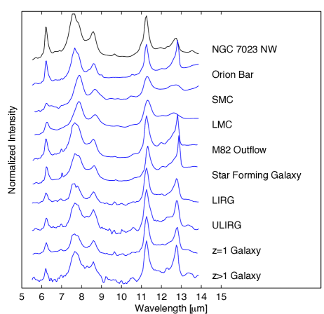
Figure 1: Mid-infrared spectra of the interstellar medium in regions of the Milky Way and other galaxies obtained with the IRS instrument onboard the Spitzer Space Telescope. The Orion Bar is a UV irradiated molecular ridge in the Orion star-forming region. SMC and LMC refer to the Small and Large Magellanic Clouds. M82 is a nearby galaxy with intense star formation activity. The Luminous and Ultraluminous Infrared Galaxies (respectively LIRG and ULIRG) spectra are templates obtained by stacking the spectra from a large sample of galaxies (Dasyra et al. 2009). The $0<z<1$ and $1<z<2$ spectra, where z means redshift, were obtained by stacking the spectra from a large sample of galaxies (Dasyra et al. 2009) and are presented in their rest frame. These spectra represent galaxies in the early universe.

The spectra in Figure 1 span a wide range of objects, physical conditions, star formation activity/history, age, metallically, and mass. While showing small differences in detail, regardless of their environment, all spectra resemble each other in peak position and profile and are dominated by emission features centered around 6.2, 7.7, 8.6, 11.2 and 12.7 $\mu$m. The similarity between the spectra in Figure 1 is striking, with an average correlation coefficient of 0.8. This high correlation between observed spectra implies universal properties for the carrier(s) of these AIBs. In the following, we will attempt to reproduce these observations using quantum chemically calculated spectra and to explain the universal character of the observed AIB spectrum. The black spectrum in Figure 1 is NGC 7023-NW and will be used as the typical PAH spectrum for comparison to the models in the remainder of the text.This is an environment with an intense UV radiation field, representative of star-forming regions, which dominate the mid-IR emission of galaxies.

3 Results

3.1 NASA Ames PAH IR Spectroscopic Database

Version 1.32 of the NASA Ames PAH IR Spectroscopic Database is used, which contains 659 computed PAH spectra (Bauschlicher et al. 2010; Boersma et al. 2014). From these, 548 were selected, excluding those spectra from PAHs containing oxygen, magnesium, silicon and iron, as these are commonly not considered to exist at high abundances, if at all, in space. The selected set holds the spectra from a wide variety of PAHs; PAHs of different sizes ($9\leq N_{\rm C}\leq 384$), ionization states (-,0,+,++,+++), and geometries. A discussion on biases in the database can be found in Appendix A.

In order to compare astronomical AIB emission spectra with computed absorption spectra from the NASA Ames PAH IR Spectroscopic Database, an emission model is required. Here, the single photon, single PAH emission model is adopted, which is fully implemented by the AmesPAHdbIDLSuite (Bauschlicher et al. 2010; Boersma et al. 2014). Each PAH is given an internal vibrational energy of 6.0 eV and put through the entire emission-cooling cascade.

While the choice of emission profile and its width will not affect our general result, they do become important when making the direct comparison to astronomical observations. Here Lorentzian emission profiles are chosen with a fixed width of 15 cm^-1. However, anharmonicity will shift the peak position and broaden the bands. The exact amount of this shift and broadening is dependent on the specific molecule, temperature, and vibrational mode (Cherchneff et al. 1992; Cook & Saykally 1998; Joblin et al. 1995; Pech et al. 2002; Oomens et al. 2003). It is this complexity that restricts the emission model from dealing with anharmonicity in detail. However, an overall redshift of 15 cm^-1 is applied, which is consistent with shifts for the out-of-plane bending modes of PAHs at $\sim$900 K measured in the laboratory (Joblin et al. 1995; Pech et al. 2002). The resulting emission spectra are presented in the top panel of Figure 2 and illustrate the diversity in spectral features between PAH species.

3.2 Database Mixtures

From the 548 PAH emission spectra calculated in Section 3.1, 1000 random mixtures were created by assigning each 5-15 $\mu$m PAH spectrum a random abundance between 0 and 1 and then averaging. The results are presented in the left panel of Figure 2. The similarity between the 1000 mixtures is astonishing, with an average correlation coefficient of 0.96 (see Appendix B).

We can continue this analysis for the different charge states of the PAH species. From the 254 and 222 PAH cations and neutrals, respectively, we create 1000 random mixtures of each. The middle and right panels of Figure 2 present these mixtures for the PAH cations and neutrals, respectively. Consistent with the results from the entire dataset, the mixed spectra are extremely similar. Yet unlike the full dataset, clearcut difference appear between the two separate charge sets. These differences between neutral and cations are in agreement with those mentioned earlier (Szczepanski & Vala 1993; Hudgins & Allamandola 1995b, a; Allamandola et al. 1999). We refer to the average spectrum from the 1000 mixtures calculated above as “kernel” spectra.

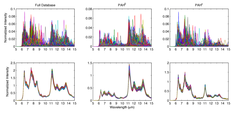
Figure 2: The effect of randomly mixing 5-15 $\mu$m PAH spectra Left column: Upper panel: Calculated emission spectra for all of the 548 pure or nitrogenated PAH species from the NASA Ames PAH IR Spectroscopic Database (Bauschlicher et al. 2010; Boersma et al. 2014). Each color represents the spectrum of a different PAH species. The width of the PAH bands has been set to 15 cm^-1 and a redshift of 15 cm^-1 has been applied to mimic some effects of anharmonicity. These parameters have been selected to convert the database spectra from absorption into emission spectra and are close to values observed in the laboratory (Appendix A). Lower panel: 1000 random mixtures of the 548 different PAH emission spectra in the upper panel. Each color represents one of the 1000 mixtures, each mixture containing 548 species in different abundances. Middle column: Same as left column but considering only PAH cations (PAH⁺). Right column: Same as left column but considering only PAH neutrals (PAH⁰).

4 Analysis

4.1 Comparison with Observations

In the left panel of Figure 3, we compare the kernel spectra directly to astronomical observations of the reflection nebula NGC 7023; representative of the galactic ISM. The kernel spectrum of the full database matches the salient characteristics of the observed NGC 7023 spectrum well. Some of the discrepancies between the kernel spectra and observations can be attributed to the employed emission model, which is unable to treat anharmonicity (Basire et al. 2011). In addition, we do not reproduce a strong 12.7 $\mu$m feature, which is observed in most PAH spectra. Recent work attributes this feature to long chains of aliphatic PAHs (Candian et al. in prep.), which are under-represented in the database. Similarly, the 6.2 $\mu$m feature has been attributed to curved PAHs (Galue 2014), which are not yet represented in the database, and thus we cannot reproduce this feature.

Figures. 3b) & 3c) compare the kernel spectra for PAH cations and neutrals, respectively, with the corresponding spectra extracted from NGC 7023 separated using blind signal separation techniques (Rapacioli et al. 2005; Berné et al. 2007; Berne et al. 2010) (Appendix D). The agreement between the PAH kernel spectra and the blind signal separations components extracted from the observations, is striking for both neutral and cationic PAHs. We find a correlation coefficient of 0.74, comparing the 5-15 $\mu$m regions, and a coefficient of 0.94 if we exclude the 6.2 and 12.7 $\mu$m features.

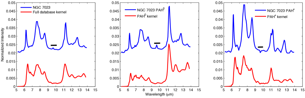
Figure 3: Comparison of the 5-15 $\mu$m kernel spectra (Figure2) with the observations and components from a blind signal decomposition (BSS) of the reflection nebula NGC 7023. Left Panel: Comparison of the spectrum of NGC 7023 (blue) and the kernel spectrum resulting from the 1000 random mixtures of 548 computed PAH spectra. Middle Panel: Comparison between the astronomical neutral PAHs (PAH⁰) spectrum extracted from the observations of NGC 7023 (blue) using blind signal separation techniques (Rapacioli et al. 2005; Berné et al. 2007; Berne et al. 2010;Appendix D) and the kernel spectrum (red) resulting from random mixtures of computed neutral PAH spectra. Right Panel: Same as the middle panel but now for cation PAH species (PAH⁺). In all panels, solid black line indicates the pure rotational line of the molecular hydrogen molecule at 9.7 $\mu$m.

4.2 Statistical Analysis

In order to determine the minimum number of PAH species necessary to reproduce the full database kernel spectrum with spread comparable to observations, we conduct a statistical analysis. The details of this analysis can be found in Appendix C. The general procedure involves making many mixtures (as in Section 3.2), but varying the number of PAH species included in the mixtures, from 10-100. The analysis shows that by increasing the number of species in the sample, the resulting variations between the spectra decrease. It can be shown that with $\sim$ 30 or more PAHs in the mixture, the variations in the modeled spectra are within the amount observed int the AIBs. This analysis relies on a biased sample (database and observations) and an arbitrary norm, therefore the number 30 should not be considered as a sharp limit (see appendix C for details). Nonetheless, these results indicate, that a large number of PAH molecules can reproduce the AIBs.

5 Discussion

The results presented here show that any random mixture of many (more than $\sim$30) PAH molecules, given the limitations of the adopted emission model, can reproduce the salient spectral characteristics of the astronomical AIB spectrum to a remarkable degree. In this respect, the similarity between the AIB spectra observed across the Universe can be understood as being due to the presence of a sufficient number of varying interstellar PAHs (on the order of 30), which, when emitting together, produce the Universal ’kernel’ spectrum. While this spectrum can only arise from a mixture containing a sufficient number of varying PAH species, given the limitations of the observational spectra and databases, it does not seem to require the presence of a specific PAH. Instead, the observed variations can be attributed to changes in the overall, global, characteristics of the PAH population such as charge, structure, and so on.

Additionally, this implies it will be challenging to identify a particular interstellar PAH by any other spectroscopic means, in particular by electronic transitions in the UV to near infrared range, far-IR vibrational bands, or pure-rotational lines at millimeter wavelengths (for PAHs with a dipole moment) as spectral signatures are damped by a factor that is – to first order – proportional to the number of different species. This is a large part of the reason why attempts to identify these signatures have not succeeded so far (Mulas et al. 2006; Pilleri et al. 2009; Gredel et al. 2011). To make progress in these other wavelength regions, where specific PAH identification is possible, will require much higher signal-to-noise observations coupled with very high precision laboratory spectroscopy.

Recently, the idea that PAH could be the carriers of the AIBs was contested by Kwok & Zhang (2011) who propose that, instead, these same bands arise from complex organic solids with disorganized structures. This latter work, based on an analysis of archival infrared spectroscopic data, relies on an empirical decomposition of the observed spectra and does not include theoretical emission cross sections nor any modeling of the emission mechanism for the proposed carriers. Our analysis instead shows that random mixtures of many ($>30$) theoretical emission spectra of PAH molecules correlate with observations to a high degree. In addition, with our model, we are able to explain the remarkable consistency of the shape of the PAH spectrum in the universe as well as the subtle spectral variations observed in the Milky Way. On this solid basis, we conclude that PAHs are better candidates for the AIBs than the structures proposed by Kwok & Zhang (2011).

Finally, as properties such as ionization are tangible and closely linked to local conditions (i.e., UV-field, and electron density and the temperature of the gas), improved knowledge of PAHs and their emission mechanism will improve the use of AIBs as probes of local and distant astrophysical environments. Future instruments, such as the mid-infrared instrument (MIRI) on the James Webb Space Telescope (JWST), and the Mid-infared E-ELT Imager and Spectrograph (METIS) on the European Extremely Large Telescope (E-ELT) will open up the wealth of information hidden in the details of the AIB spectra. Although these instruments will not be able to identify specific PAH species due to the band overlap, they will be able to trace in finer details the general properties of the PAH family and to relate these properties to local physical conditions.

Appendix A Database Biases

The content of the computed part of the NASA Ames PAH IR Spectroscopic Database has some intrinsic biases (Bauschlicher et al. 2010; Boersma et al. 2014). These biases originate historically from a limit in available computational power, that smaller PAH species (N${}_{C}<20$) are more easily calculated, and a focus on astrophysically relevant species, i.e., ’pure’, cata-condensed, neutral and singly positively ionized PAH species (Tielens 2008). The bias towards small PAHs in the database is somewhat negated by the physics of the PAH emission process and the wavelength range considered here (5-15 $\mu$m). Small PAHs get significantly hotter than their larger counterparts upon absorbing the same photon energy. This pushes more of the emission blue of the wavelength region considered here. Similarly for large PAHs (N${}_{C}>80$), which stay significantly cooler, more of the emission is pushed red of the wavelength region considered here. From a stability standpoint, the family of cata-condensed, compact PAHs is very stable and hence more likely to survive the rigors of interstellar space (Allamandola et al. 1985). These species are well represented in the database. The database does undersample dehydrogenated PAHs, both in the levels of dehydrogenation and the possible permutations. However, it has been shown that the removal of only one or two hydrogens from cata-condensed PAHs does not alter the spectrum much and that such fully dehydrogenated species in space are probably rare (Bauschlicher & Ricca 2013). Variations in peripheral hydrogen adjacencies are reflected by variations in the 10-15 $\mu$m region of the PAH spectrum (Hony et al. 2001). As PAHs become increasingly larger, while remaining compact, they obtain more and more straight edges. This is reflected in their spectra by a strong 11.2 $\mu$m feature. Adding more irregular PAHs to the database can alleviate some of the current bias towards compact, straight edged PAHs in the database. Of all studied hetero atom substitutions, nitrogen has shown to be the most viable candidate, as its inclusion does not affect PAHs stability, nitrogen is abundant in the circumstellar shells around carbon rich AGB stars (Allamandola et al. 1985, 1989; Frenklach & Feigelson 1989), the place where PAHs are thought to be formed (Boersma et al. (2006), and references therein) and their known presence in meteorites (Hayatsu et al. 1977). Other substitutions either have little effect (e.g., silicon, magnesium) or significantly disrupt the aromatic network, and therefore reduce the stability of the PAH, e.g., oxygen (Hudgins et al. 2005). Singly charged PAH anions are well represented in the database for the larger PAH species. Considering detailed charge balance, doubly charged PAH cations only become important in the more extreme astrophysical environments and higher ionization states can safely be ignored. These and other considerations regarding database biases and their astrophysical relevance have also been discussed in Boersma et al. (2013). Our database mixed spectra are affected by these biases. The region in the spectrum most affected is the 10-15 $\mu$m range due to the underrepresentation of irregular PAHs. This could also explain the disparity between the observations and the database mixtures in these regions e.g., the weak 12.7 $\mu$m feature.

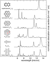
Figure 4: Structure and DFT computed 5-15 $\mu$m vibrational infrared spectra of a selection of PAHs. PAHs are a class of carbonaceous molecules, which form a skeleton where carbon atoms are arranged in a honeycomb structure with hydrogen atoms sitting on the periphery. Additional atoms, such as Nitrogen, also can be present in the skeleton. For each species, the chemical formula, simple name (if it exists), and the corresponding mid-infrared spectrum calculated by DFT at 0 K are given. All data are taken from the NASA Ames PAH IR Spectroscopic Database (Bauschlicher et al. 2010; Boersma et al. 2014).

Appendix B Correlation between the 1000 mixtures

Figure B1 shows the probability density function (PDF) of the correlation matrix of the 1000 mixtures (Figure 2 Left panel). The peak, average and median correlation coefficients are shown in blue, red and green, respectively. The 1-sigma variation around the mean is shown in yellow. The peak of the PDF (the most likely correlation) is found at 0.96 and the standard deviation is 0.023, i.e. 85% of the correlations fall between 0.94 and 0.98. Only 4% of the correlations are below 0.9. The distribution is a sharp, narrow distribution, showing without a doubt that random PAH mixtures are indeed very alike.

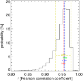
Figure 5: Probability density function of the correlation coefficients between the average 5-15 $\mu$m spectra from 1000 mixtures of 548 species with random abundances between 0-1. The peak, average and median correlation coefficients are shown in blue, red and green, respectively. The 1-sigma variation around the mean is shown in yellow.

Appendix C Statistical Analysis Details

First we concentrate on the database and apply the following procedure:

1. Randomly select $r$ spectra from the database.

2. Create m random linear combinations (mixtures) of the $r$ spectra by assigning each spectrum a random abundance between 0 and 1 such that;

   X=AS (1)

   Where $X$ is an $m\times n$ matrix holding $m$ number of mixed spectra over $n$ wavelength bins, $A$ is an $m\times r$ abundance matrix, containing random numbers between 0 and 1, and $S$ is a $r\times n$ matrix holding the original set of database spectra. For this analysis we set $m$ to 100, creating 100 random mixtures each time.

3. Repeat steps (1)-(2) $p$ times, randomly selecting a new set of $r$ PAH spectra each time (here we vary $r$ between 10 and 100). Thus, $p$ spectra in matrix $X$ are created, which we will denote as $X_{i}$. We use $p$=100 for this analysis. This means that there are $m$ random mixtures of $r$ spectra, and we re-select and re-mix those $r$ spectra $p$ times.

4. We find the maximum, minimum, and mean value of the spectra with index $i$, $X_{i}$, in the $X$ matrix and for every wavelength bin, $\lambda$. From these values we create three spectra, $S_{max}(\lambda)$, $S_{min}(\lambda)$, and $S(\lambda)$. The spectra $S_{max}(\lambda)$ and $S_{min}(\lambda)$ represent the boundaries within which any spectrum ($X_{i}$) falls. The mean spectrum $\bar{S(\lambda)}$ is the kernel spectrum for that particular set of $m\times p$ mixed spectra.

5. We calculate the Euclidian distance from the minimum and maximum spectra with respect to the mean:

   $$N_{min}=\sqrt{\sum_{\lambda=1..n}(S_{min}-\bar{S})^{2}}$$ (2)

   $$N_{max}=\sqrt{\sum_{\lambda=1..n}(S_{max}-\bar{S})^{2}}$$ (3)

   and we define $N_{r}$ as

   $$N_{r}=N_{min}+N_{max}$$ (4)

   which is a measurement of the maximum variation in the mixtures for each set of $r$ spectra.

Now we consider the observations and calculate $N_{obs}$ using the following steps:

1. Subtract a linear baseline (corresponding to the emission from another dust component) for each observed spectrum

2. Out of the 10 observed rest-frame spectra, define a minimum, maximum, and mean at each wavelength bin.

3. Similarly to step 4 in the database analysis, we find the maximum, minimum, and mean value of the observed spectra with index $i$, $X_{i}$, in the $X$ matrix and for every wavelength bin, $\lambda$. From these values we create three spectra, $S_{obs,max}(\lambda)$, $S_{obs,min}(\lambda)$, and $S_{obs}(\lambda)$. The spectra $S_{obs,max}(\lambda)$ and $S_{obs,min}(\lambda)$ represent the boundaries within which any of the observed spectra ($X_{i}$) fall. The mean spectrum $S_{obs}(\lambda)$ is the average of the particular set of rest-frame observations presented in Figure 1.

   Similarly to (6) for the database spectra, we define:

   $$N_{obs,min}=\sqrt{\sum_{n}(S_{obs,min}-\bar{S}_{obs})^{2}}$$ (5)

   $$N_{obs,max}=\sqrt{\sum_{n}(S_{obs,max}-\bar{S}_{obs})^{2}}$$ (6)

   $$N_{obs}=N_{obs,min}+N_{obs,max}$$ (7)

C.1 Comparison between database and observations statistics

In Figure 6, we present the results of the statistical analysis in a graphical way. The top panel of Figure 6 shows the shaded regions between $S_{min}$ and $S_{max}$, which highlights the boundaries of the $m\times i$ mixtures of $r$ spectra. The lightest grey shaded region represents $r=10$, and increasingly darker greys represent $r=20-90$. The red region is where $r=100$ and the black region is when $r=548$, the whole database. It appears clearly that, by increasing the number of species in the sample, the resulting variations between the kernel spectra decrease. This can be investigated more quantitatively, by following the evolution of the norm $N_{r}$ as a function of the number of species present in the mixture $r$. This is done in the bottom panel of Figure 6 where the decrease of $N_{r}$ can be seen clearly. One way to compare the variations of the observed AIB spectrum with those present in the kernel spectra, is to compare $N_{r}$ with $N_{obs}$ which has a constant value reported in Figure 6. When $N_{r}<N_{obs}$, the spectral variations (in terms of Euclidian norm as defined in Appendix C) of the database mixture are within the spectral variations observed in PAH. This happens when $r>30$ (Figure 6).

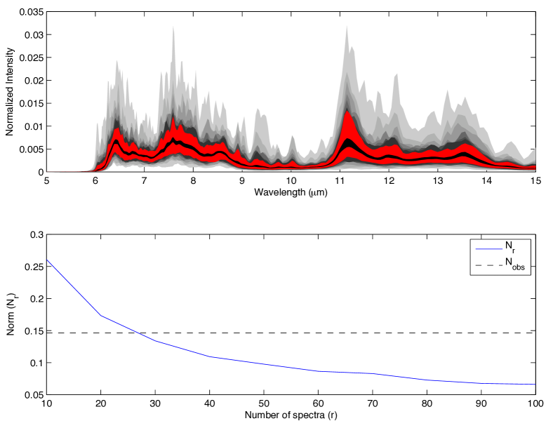
Figure 6: Top panel: range of variations in the kernel spectra as a function of the number of PAH species considered in the mixture: 10 species (light grey) through 90 species (dark grey). In red is the range for 100 species and in black the range for 548 species. Bottom panel: evolution of the norm $N_{r}$ which captures the variations in the kernel spectra (blue line) and the norm $N_{obs}$ which captures the variations in the observations (see text for details).

Appendix D Blind Signal Separation

Blind Signal Separation is commonly used to restore a set of unknown “source” signals from a set of observed signals which are mixtures, or combinations, of these original source signals, with unknown mixture parameters Hyvarinen et al. (2001). Several methods and algorithms exist in in the literature. The astronomical PAH cation and neutral spectra presented in this Letter were obtained with Lee and Seung’s non-negative matrix factorization (Lee & Seung 2001, NMF). NMF was applied to data of the reflection nebula NGC 7023 obtained with the Infrared Spectrograph onboard the Spitzer Space Telescope. Details on the procedure can be found in Berne et al. (2010).

References

- Allamandola et al. (1999) Allamandola, L. J., Hudgins, D. M., & Sandford, S. A. 1999, ApJ, 511, L115
- Allamandola et al. (1985) Allamandola, L. J., Tielens, A. G. G. M., & Barker, J. R. 1985, ApJ, 290, L25
- Allamandola et al. (1989) Allamandola, L. J., Tielens, A. G. G. M., & Barker, J. R. 1989, ApJS, 71, 733
- Basire et al. (2011) Basire, M., Parneix, P., Pino, T., Bréchignac, P., & Calvo, F. 2011, in EAS Publications Series, Vol. 46, EAS Publications Series, ed. C. Joblin & A. G. G. M. Tielens, 95–101
- Bauschlicher et al. (2010) Bauschlicher, Jr., C. W., Boersma, C., Ricca, A., et al. 2010, ApJS, 189, 341
- Bauschlicher & Ricca (2013) Bauschlicher, Jr., C. W. & Ricca, A. 2013, ApJ, 776, 102
- Berné et al. (2007) Berné, O., Joblin, C., Deville, Y., et al. 2007, A&A, 469, 575
- Berne et al. (2010) Berne, O., Tielens, A., Pilleri, P., & Joblin, C. 2010, in Hyperspectral Image and Signal Processing: Evolution in Remote Sensing (WHISPERS), 2010 2nd Workshop on, 1–4
- Boersma et al. (2014) Boersma, C., Bauschlicher, Jr., C. W., Ricca, A., et al. 2014, ApJS
- Boersma et al. (2013) Boersma, C., Bregman, J. D., & Allamandola, L. J. 2013, ApJ, 769, 117
- Boersma et al. (2006) Boersma, C., Hony, S., & Tielens, A. G. G. M. 2006, A&A, 447, 213
- Bregman et al. (1989) Bregman, J. D., Allamandola, L. J., Witteborn, F. C., Tielens, A. G. G. M., & Geballe, T. R. 1989, ApJ, 344, 791
- Cherchneff et al. (1992) Cherchneff, I., Barker, J. R., & Tielens, A. G. G. M. 1992, ApJ, 401, 269
- Cook & Saykally (1998) Cook, D. J. & Saykally, R. J. 1998, ApJ, 493, 793
- Dasyra et al. (2009) Dasyra, K. M., Yan, L., Helou, G., et al. 2009, ApJ, 701, 1123
- Draine & Li (2007) Draine, B. T. & Li, A. 2007, ApJ, 657, 810
- Frenklach & Feigelson (1989) Frenklach, M. & Feigelson, E. D. 1989, ApJ, 341, 372
- Galliano et al. (2008) Galliano, F., Madden, S. C., Tielens, A. G. G. M., Peeters, E., & Jones, A. P. 2008, ApJ, 679, 310
- Galue (2014) Galue, H. A. 2014, Chem. Sci.,
- Gredel et al. (2011) Gredel, R., Carpentier, Y., Rouillé, G., et al. 2011, A&A, 530, A26
- Hayatsu et al. (1977) Hayatsu, R., Matsuoka, S., Anders, E., Scott, R. G., & Studier, M. H. 1977, Geochim. Cosmochim. Acta., 41, 1325
- Hony et al. (2001) Hony, S., Van Kerckhoven, C., Peeters, E., et al. 2001, A&A, 370, 1030
- Houck et al. (2004) Houck, J. R., Roellig, T. L., van Cleve, J., et al. 2004, ApJS, 154, 18
- Hudgins & Allamandola (1995a) Hudgins, D. M. & Allamandola, L. J. 1995a, The Journal of Physical Chemistry, 99, 3033, pMID: 11538457
- Hudgins & Allamandola (1995b) Hudgins, D. M. & Allamandola, L. J. 1995b, The Journal of Physical Chemistry, 99, 8978, pMID: 11538316
- Hudgins et al. (2005) Hudgins, D. M., Bauschlicher, Jr., C. W., & Allamandola, L. J. 2005, ApJ, 632, 316
- Hyvarinen et al. (2001) Hyvarinen, A., Karhunen, J., & Oja, E. 2001, in Independent Component Analysis, ed. Wiley
- Joblin et al. (1995) Joblin, C., Boissel, P., Leger, A., D’Hendecourt, L., & Defourneau, D. 1995, A&A, 299, 835
- Joblin & Tielens (2011) Joblin, C. & Tielens, A. G. G. M., eds. 2011, EAS Publications Series, Vol. 46, PAHs and the Universe: A Symposium to Celebrate the 25th Anniversary of the PAH Hypothesis
- Joblin et al. (1996) Joblin, C., Tielens, A. G. G. M., Geballe, T. R., & Wooden, D. H. 1996, ApJ, 460, L119
- Kwok & Zhang (2011) Kwok, S. & Zhang, Y. 2011, Nature, 479, 80
- Lee & Seung (2001) Lee, D. D. & Seung, H. S. 2001, in NIPS, ed. MIT press, Vol. 13, 556
- Li & Draine (2012) Li, A. & Draine, B. T. 2012, ApJ, 760, L35
- Mattioda et al. (2005) Mattioda, A. L., Allamandola, L. J., & Hudgins, D. M. 2005, ApJ, 629, 1183
- Mulas et al. (2006) Mulas, G., Malloci, G., Joblin, C., & Toublanc, D. 2006, A&A, 456, 161
- Oomens et al. (2003) Oomens, J., Tielens, A. G. G. M., Sartakov, B. G., von Helden, G., & Meijer, G. 2003, ApJ, 591, 968
- Pech et al. (2002) Pech, C., Joblin, C., & Boissel, P. 2002, A&A, 388, 639
- Pilleri et al. (2009) Pilleri, P., Herberth, D., Giesen, T. F., et al. 2009, MNRAS, 397, 1053
- Rapacioli et al. (2005) Rapacioli, M., Joblin, C., & Boissel, P. 2005, A&A, 429, 193
- Siebenmorgen et al. (2014) Siebenmorgen, R., Voshchinnikov, N. V., & Bagnulo, S. 2014, A&A, 561, A82
- Szczepanski & Vala (1993) Szczepanski, J. & Vala, M. 1993, Nature, 363, 699
- Tielens (2008) Tielens, A. G. G. M. 2008, ARA&A, 46, 289
- Werner et al. (2004) Werner, M. W., Roellig, T. L., Low, F. J., et al. 2004, ApJS, 154, 1