Competing phases, phase separation and co-existence in the extended one-dimensional bosonic Hubbard model

Abstract

We study the phase diagram of the one-dimensional bosonic Hubbard model with contact ($U$) and near neighbor ($V$) interactions focusing on the gapped Haldane insulating (HI) phase which is characterized by an exotic nonlocal order parameter. The parameter regime ($U$, $V$ and $\mu$) where this phase exists and how it competes with other phases such as the supersolid (SS) phase, is incompletely understood. We use the Stochastic Green Function quantum Monte Carlo algorithm as well as the density matrix renormalization group to map out the phase diagram. Our main conclusions are that the HI exists only at $\rho=1$, the SS phase exists for a very wide range of parameters (including commensurate fillings) and displays power law decay in the one body Green function. In addition, we show that at fixed integer density, the system exhibits phase separation in the $(U,V)$ plane.

I Introduction

The bosonic Hubbard model (BHM) has continued to attract interest since its introduction by Fisher et al. fisher89 . This interest stems from the versatility of the model and its use in understanding many physical phenomena such as adsorption of bosonic atoms on surfacesbatrouni94a , effect of disorder on superfluids and the appearance of the compressible Bose glass phase fisher89 , quantum phase transitions between strongly correlated exotic phases etc. In addition, in the hardcore limit, the BHM can be mapped onto Heisenberg spin models and thus offers the opportunity to study these important systems under various conditions. Study of the BHM intensified with the experimental realization of Bose-Einstein condensates and the ability to load them in optical lattices greiner02 . Under experimentally realizable conditions, these systems are described by the BHM and its extensions jaksch99 with highly tunable parameters and in one, two and three dimensions.

An increasing focus of the physics of strongly correlated quantum systems over the last several years has been the existence of unconventional phases and phase transitions. In addition to well studied Mott insulating behavior caused by an on-site repulsion, or charge order driven by a near-neighbor repulsion, usurping superfluidity, more exotic scenarios are realized in which different types of order are simultaneously present, or entirely new patterns arise. An additional motivation for studying the extended one-dimensional BHM is that it provides a concrete Hamiltonian in which this physics can be examined with powerful numerical methods.

In its simplest form which has only on-site contact interactions, the ground state of the BHM exhibits two phases fisher89 . At integer filling and strong repulsion, boson displacement is sterically suppressed and the system is in an incompressible Mott insulating (MI) phase which is replaced by a superfluid (SF) phase at weak coupling. At incommensurate fillings, the system is always SF. Extending this model with the addition of longer range interactions or anisotropic hopping terms leads to new exotic phases. For example, extensive quantum Monte Carlo (QMC) simulations have shown that a strong enough near neighbor repulsion can lead to insulating incompressible density wave order (CDW) at integer and half odd integer fillings. Doping these phases can lead to phase separation or to supersolid (SS) phases batrouni95 ; batrouni00 ; goral02 ; wessel05 ; boninsegni05 ; sengupta05 ; otterlo05 ; batrouni06 ; yi07 ; suzuki07 ; dang08 ; pollet10 ; capogrosso10 .

The possibility of mapping the BHM onto a Heisenberg model invites the question of whether the same phases of the latter are present for the former. For example, odd integer Heisenberg spin systems in one-dimensional lattices can exhibit the exotic Haldane phase which is a gapped phase characterized by a non-local (string) order parameter haldane83 ; dennijs89 . It was shown for the extended one-dimensional BHM with near and next near neighbor interactions that, at an average filling of one particle per site, the system can be mapped approximately onto the spin-$1$ Heisenberg model and admits a Haldane insulating (HI) phase sandwiched between MI and CDW phases altman06 ; altman08 . The phase diagram at unit filling for the system with only contact ($U$) and near neighbor ($V$) interactions was studied more extensively with conflicting results for the phase diagram. In Refs. [batrouni91, ; batrouni94, ] the phase diagram was shown to exhibit MI, SF and CDW phases but the HI was not found due to the very limited sizes possible to simulate at the time. Subsequently, the $(\mu,t)$ phase diagram of the extended BHM, for a fixed $V/U$ ratio, was obtained using Density Matrix Renormalization Group (DMRG) kuhner00 , but showed only evidence for MI, SF and CDW. Recent work rossini12 , also based on the DMRG, has shown the presence of the HI phase between the MI and CDW phases but found no evidence of SS at unit filling. Even more recent work minguzzi on the same model has confirmd the HI phase. Curiously, however, there seems to be no consensus on the nature of the phase in the ($U,V$) plane at unit filling for small $U$ and large $V$. References [batrouni91, ; batrouni94, ; minguzzi, ] show it to be SF while Ref. [rossini12, ] shows it to be CDW and reference [santos, ] claims it to be supersolid. We will show in this paper that it is none of the above.

The above results give rise to some questions. Does the HI exist for other integer fillings of the system or is it a special property of the unit filling case? The SS phase found in one dimension batrouni06 was obtained by doping a CDW phase: Does this phase also exist for commensurate fillings in one dimension for parameter choices similar to those in two kawashima12a and three dimensions kawashima12b ? If the SS phase exists for commensurate fillings, where is it situated in the phase diagram relative to the CDW, MI and HI phases?

Theoretical studies of this system using bosonization have also led to mixed results: The HI was obtained and characterizedaltman08 but consensus is absent on whether the SS phase exists in this model. Even though older studies did not specifically mention it Giamarchi_book or even argued that it did not exist kuhner00 , more recent studies seem to demonstrate the presence of the SS phase  Sengupta07 ; alexia , even without nearest neighbor interaction Lazarides11 , for both commensurate and incommensurate fillings. However, the precise nature of order and the decays of the relevant correlation functions are still far from settled. For instance, some studies predict that the single particle Green function decays exponentially in the SS phase while the density-density correlation function decays as a power Lee07 ; others predict that both of these correlation functions decay as powers Sengupta07 . Finally, the universality class of the transition to the SS phase remains largely unexplored.

In this paper we extend our work in Ref. [batrouni13, ] using the stochastic Green function (SGF) QMC algorithm sgf and the density matrix renormalization group (DMRG) to study the phase diagram of the one dimensional extended BHM as a function of the contact (near neighbor) interaction $U$ ($V$) and the filling. For the DMRG calculations we use the code available in the ALPS library alps . We mention that the fermionic version of this model was also studied by means of bosonization and DMRGbarbiero and a HI phase established.

The paper is organized as follows. In section II we present the model and discuss the various phases of interest and the order parameters which characterize them. In section III we present our QMC and DMRG results for the phase diagrams in the $(U,V)$ plane at fixed fillings, $\rho=1$ and $\rho=3$. We present in section IV our results for the phase diagram in the $(\mu/U,t/U)$ plane at fixed ratio $V/U=3/4$. A summary of results and conclusions is in section V.

×	$\rho_{s}$	$S(\pi)$	$\Delta_{c}$	$\Delta_{n}$	${\cal O}_{p}(L_{max})$	${\cal O}_{s}(L_{max})$
MI	$0$	$0$	$\neq 0$	$=\Delta_{c}$	$\neq 0$	$=0$
CDW	$0$	$\neq 0$	$\neq 0$	$\neq 0$	$\neq 0$	$\neq 0$
SF	$\neq 0$	$0$	$0$	$0$	$0$	$0$
HI	$0$	$0$	$\neq 0$	$\neq 0$	$0$	$\neq 0$
SS	$\neq 0$	$\neq 0$	$0$	$0$	$\neq 0$	$\neq 0$

Table 1: Order parameters characterizing various phases.

II The Model

The one dimensional extended BHM we shall study is described by the Hamiltonian,

$$H = -t\sum_{i}(a^{\dagger}_{i}a^{\phantom{\dagger}}_{i+1}+a^{\dagger}_{i+1}a^{\phantom{\dagger}}_{i})+\frac{U}{2}\sum_{i}n_{i}\left(n_{i}-1\right)$$ (1)

$$+V\sum_{i}n_{i}n_{i+1}.$$

The sum over $i$ extends over the $L$ sites of the lattice, periodic boundary conditions were used in the QMC and open conditions with the DMRG. The hopping parameter, $t$, is put equal to unity and sets the energy scale, $a_{i}^{\phantom{\dagger}}$ ($a_{i}^{\dagger}$) destroys (creates) a boson on site $i$, $n_{i}=a_{i}^{\dagger}a_{i}^{\phantom{\dagger}}$ is the number operator on site $i$, $U$ and $V$ are the onsite and near neighbor interaction parameters.

Several quantities are needed to characterize the phase diagram. It was shown recentlyval that the well-known expression of the superfluid density as a function of the fluctuations of the winding numberpollock is valid only for Hamiltonians that satisfy

$$[R,H]=\frac{i\hbar}{m}P,$$ (2)

where $R$ and $P$ are the position and momentum operators and $m$ is the mass of a boson. Here $t=\hbar^{2}/(2m{\ell}^{2})$ where $\ell$ is the lattice constant. It is straightforward to verify that Eq.(1) satisfies this condition and, therefore, the superfluid density is given bypollock

$$\rho_{s}=\frac{\langle W^{2}\rangle}{2td\beta L^{d-2}},$$ (3)

where $W$ is the winding number of the boson world lines, $d$ is the dimensionality and $\beta$ the inverse temperature. The CDW order parameter is the structure factor, $S(k)$, at $k=\pi$ where

$$S(k)=\frac{1}{L}\sum_{r=0}^{L-1}{\rm e}^{ikr}\langle n_{0}n_{r}\rangle,$$ (4)

and the momentum distribution, $n_{k}$, is given by

$$n_{k}=\frac{1}{L}\sum_{r=0}^{L-1}{\rm e}^{ikr}\langle a^{\dagger}_{0}a^{\phantom{\dagger}}_{r}\rangle.$$ (5)

The charge gap is given by,

$$\Delta_{c}(n) = \mu(n)-\mu(n-1)$$

$$= E_{0}(n+1)+E_{0}(n-1)-2E_{0}(n)$$

where $\mu(n)=E_{0}(n+1)-E_{0}(n)$ and $E_{0}(n)$ is the ground state energy of the system with $n$ particles and is obtained both with QMC and DMRG. The neutral gap, $\Delta_{n}$, is obtained using DMRG by targeting the lowest excitation with the same number of bosons. In both CDW and HI phases, the chemical potentials at both ends are set to (opposite) large enough values, in DMRG, such that the ground state degeneracy and the low energy edge excitations are lifted kuhner00 ; altman06 . With the SGF we did simulations in both the canonical and grand canonical ensembles.

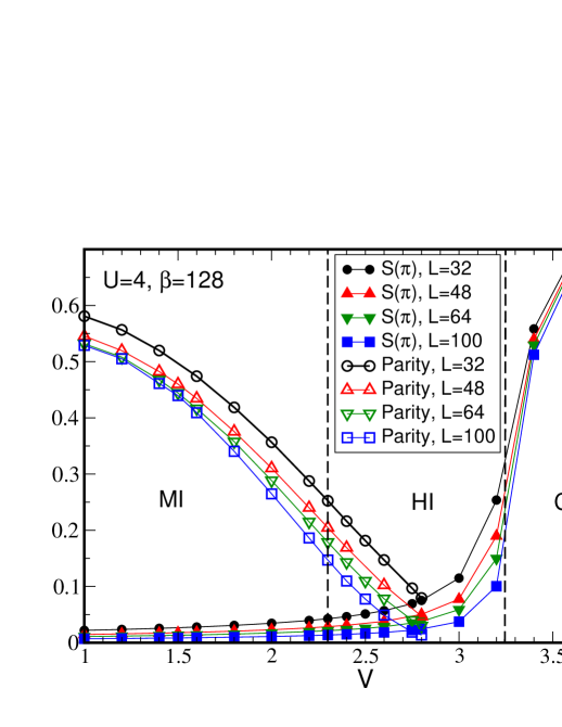
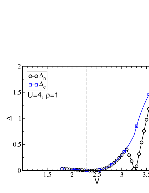
Figure 1: (color online) Top: The parity, ${\cal O}_{p}$, and CDW, $S(\pi)$, order parameters versus $V$ at fixed $U=4$ and several system sizes using QMC. By extrapolating the order parameters, $L\to\infty$, we identify two critical values, $V_{1}^{c}=2.3$, and $V_{2}^{c}=3.25$. For $V<V_{1}^{c}$, the system is in the $\rho=1$ MI; for $V>V_{2}^{c}$, the system is in the CDW phase. For $V_{1}^{c}<V<V_{2}^{c}$ (between the two vertical dashed lines), both ${\cal O}_{p}$ and $S(\pi)$ vanish as $L\to\infty$ but the string order parameter, ${\cal O}_{s}$, (not shown) remains finite. This is the HI phase. NOTE: ${\cal O}_{p}$ has been multiplied by $5$ for all sizes to render curves more visible in the figure. Bottom: The extrapolated charge, $\Delta_{c}$, and neutral, $\Delta_{n}$, gaps for the same system using DMRG. Both gaps vanish at the MI-HI transition but only the neutral gap vanishes at the HI-CDW transition, as expected. The critical values confirm the QMC results in the top panel.

For spin systems, the nonlocal Haldane string order parameter is given by,

$${\cal O}_{s}(|i-j|\to\infty) = \langle S^{z}_{i}{\rm exp}(i\theta\sum_{k=i}^{j}S^{z}_{k})S^{z}_{j}\rangle$$ (7)

where $\theta=\pi$ for the spin-$1$ system. This order parameter detects the Haldane phase where the $S_{z}=1$ and $S_{z}=-1$ alternate along the lattice and are separated by varying numbers of $S_{z}=0$ sites. In other words, the system exhibits, in this phase, long range anti-ferromagnetic order but with no characteristic momentum. In the BHM at $\rho=1$, when $U$ and $V$ are large (with $2V<U$), most sites are singly occupied. Quantum fluctuations allow some sites to be unoccupied or doubly occupied, but higher occupations are suppressed. One can therefore make the analogy with spin systems and define $S_{z}(i)\equiv\delta n_{i}=n_{i}-\rho$ ($\rho=1$) and define two nonlocal order parameters for the BHM, the string and the parity parameters:

$${\cal O}_{s}(|i-j|\to\infty) = \langle\delta n_{i}{\rm e}^{i\theta\sum_{k=i}^{j}\delta n_{k}}\delta n_{j}\rangle,$$ (8)

$${\cal O}_{p}(|i-j|\to\infty) = \langle{\rm e}^{i\theta\sum_{k=i}^{j}\delta n_{k}}\rangle.$$ (9)

In practice we take the order parameters to be ${\cal O}_{s/p}(L_{max})$ where, in QMC with PBC, $L_{max}=L/2$ and in DMRG, with OBC, $L_{max}$ is the longest distance possible before edge effects start being felt. For higher integer filling, $\rho=2,3\dots$, $\theta\neq\pi$ and has to be determined as discussed in Ref. [qin03, ].

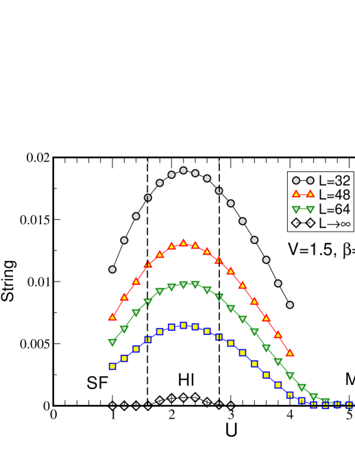
Figure 2: (color online) The string order parameter, ${\cal O}_{s}$, versus $U$ for $V=1.5$ and several sizes. Also shown are the extrapolated values giving the two critical values $U_{1}^{c}=1.6$ and $U_{2}^{c}=2.8$. For $U_{1}^{c}\leq U\leq U_{2}^{c}$ (the interval between the vertical dashed lines) the system is in the HI. For $U<U_{1}^{c}$, the system is in the SF phase and for $U>U_{2}^{c}$, it is in the MI phase.

The various thermodynamically stable phases that may appear in the system are characterized by the above quantities and are summarized in Table 1. To explore the possibility of phase separation (PS), it is not enough to look at order parameters since if the system is in a phase separated state (a mixture of two or more thermodynamic phases), there will be contributions from the order parameters of all the phases present. To preclude or confirm the presence of phase separation, we study the behavior of the density $\rho$ as a function of the chemical potential, $\mu$, and also the density profile in the system.

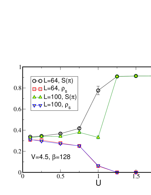
Figure 3: (color online) The superfluid density, $\rho_{s}$, and CDW order parameter $S(\pi)$ as functions of $U$ at fixed $V=4.5$ and $\rho=1$. For $U>1$: $\rho_{s}=0$ and $S(\pi)\neq 0$ indicate a CDW phase. For $U\lesssim 1$: $\rho_{s}\neq 0$ and $S(\pi)\neq 0$ suggest the possibility of a supersolid phase.

III Phase diagrams at fixed fillings

We start with the phase diagram in the ($U,V$) plane at fixed unit density. To map out the phase diagrams, we fix the filling at a commensurate value (here we focus on $\rho=1$ and $\rho=3$) and we fix one of the interaction parameters, $U$ or $V$, while the other is varied. The physical quantities discussed above ($\rho_{s}$, $S(k=\pi)$, ${\cal O}_{p}$, ${\cal O}_{s}$) are calculated and the various phases deduced from Table 1. For example, in the top panel of Fig. 1 we show ${\cal O}_{p}$ and $S(\pi)$ as functions of $V$ for the system at $\rho=1$ and fixed $U=4$ and several lattice sizes. Extrapolating these quantities to $L\to\infty$ yields the two critical values $V^{c}_{1}=2.3$, where ${\cal O}_{p}$ vanishes, and $V^{c}_{2}=3.25$ where $S(\pi)$ becomes nonzero. For all $V$ at $U=4$, $\rho_{s}=0$ (not shown in Fig. 1) and, therefore, there is no SF phase at $U=4$. The string order parameter, ${\cal O}_{s}$, vanishes for $V<V^{c}_{1}$ (not shown in the figure) and takes on a finite value for $V>V^{c}_{1}$. According to Table 1, this means that for $V<V^{c}_{1}$ the system is in the MI phase; for $V^{c}_{1}<V<V^{c}_{2}$ the system is in the HI phase and for $V>V^{c}_{2}$, the system enters the CDW phase.

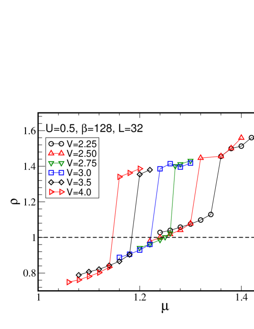
Figure 4: (color online) The density, $\rho$, as a function of the chemical potential, $\mu$, for several values of the near neighbor interaction, $V$, at fixed contact interaction, $U=1/2$. For all values of $V$ there is a discontinuous jump in $\rho(\mu)$ indicating a first order phase transition. For $V\geq 3$, the $\rho=1$ value (indicated by the dashed line) is inside the jump. This means that there is no thermodynamically stable phase with $\rho=1$ for these values of $V$. This figure was obtained with QMC simulations in the grand canonical ensemble.

These transitions can also be seen in the behavior of $\Delta_{c}$ and $\Delta_{n}$, the charge and neutral gaps, shown in the lower panel of Fig. 1 as functions of $V$ at $\rho=1$ and $U=4$. These are the extrapolated gap values, i.e., $L\rightarrow\infty$, from the DMRG results obtained for sizes ranging from $L=64$ to $L=256$. We see that at the MI-HI transition, $V=2.3$, both gaps vanish and at the HI-CDW transition, $V=3.25$, $\Delta_{n}$ vanishes while $\Delta_{c}$ does not. This behavior is expectedaltman08 and the DMRG values agree with those obtained via QMC (top panel Fig. 1).

The behavior of the string order parameter is shown in Fig. 2 as a function of $U$ for fixed $V=1.5$ and for several sizes. Also shown are the extrapolated values using ${\cal O}(L)={\cal O}(L\to\infty)+{\rm const./L}$ and demonstrating that for $1.6<U<2.8$, ${\cal O}_{s}$, although small, is nonvanishing. Therefore, the system is in the HI in this interval. For $U<1.6$ the system is SF since $\rho_{s}\neq 0$. For $U>2.8$, upon examining the other quantities such as ${\cal O}_{p}$ (nonzero) and $\rho_{s}$ (vanishes) we conclude that the system is in the MI phase.

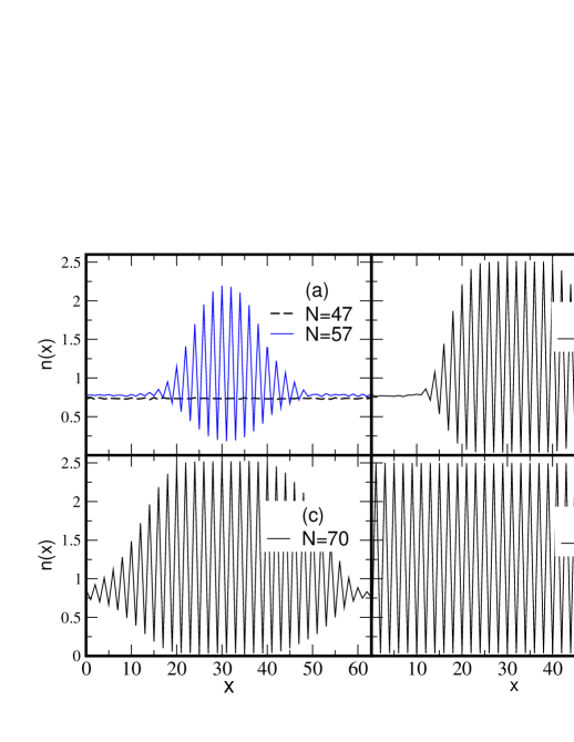
Figure 5: (color online) When, in a canonical simulation, the number of particles is fixed at a value which corresponds to a thermodynamically unstable phase, the system undergoes phase separation. In this figure, we show QMC results for $L=64$, $U=1/2$ and $V=4.5$. The phase with $N=47$ particles, dashed horizontal line in (a), is seen to be uniform and corresponds to the SF phase. Adding a few particles, however, destabilizes the system as when there are $N=57$ particles. As more particles are added, the size of the region displaying CDW increases as is seen in (b) for $N=64$ and (c) for $N=70$. In (d), with $N=81$ the system appears to be entirely CDW. However, this CDW region is in fact a supersolid. One way to see that is to notice that the density oscillates between $0$ and $2.5$. Also, the system in (d) exhibits both long range density order (CDW) and non-vanishing superfluid density. Note: In the QMC simulation, the CDW region does not always appear in the same place. Since these simulations are done with periodic boundary conditions, we have centered these regions to facilitate comparison.

The behavior of the system in the region at small $U$ and large $V$ is shown in Fig. 3 for $V=4.5$. For $U>1$, $\rho_{s}=0$ and $S(\pi)\neq 0$ signalling the presence of CDW. On the other hand, for $U\lesssim 1$, both $\rho_{s}$ and $S(\pi)$ are nonzero. This simultaneous finiteness of $S(\pi)$ and $\rho_{s}$ seems to indicate that the system is in the supersolid phase. To confirm this, however, one must show that this is a thermodynaimcally stable phase and not a mixture of two phases. To this end, we show in Fig. 4 the density, $\rho$, as a function of the chemical potential, $\mu$, for several values of $V$ and fixed $U=1/2$. All these curves, which were obtained by QMC in the grand canonical ensemble, exhibit discontinuous jumps in the density at critical values of $\mu$ which depend on $V$. This shows that, for these values of $U$ and $V$, the system exhibits a first order phase transition. Furthermore, it is clear from Fig. 4 that for $V\geq 3$ (and $U=1/2$) the discontinuous jump in $\rho$ includes the value $\rho=1$. This means that if the number of particles is fixed at $\rho=1$, i.e. if one considers the canonical ensemble, then for $U=1/2$ and $V\geq 3$, the system undergoes phase separation.

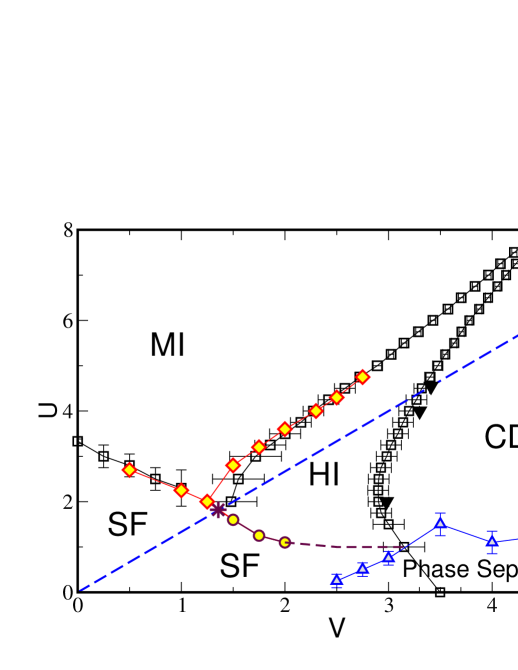
Figure 6: (color online) The phase diagram in the ($U,V$) plane for $\rho=1$. The open squares are the results of Ref. rossini12, , all other symbols are results of our QMC simulations. Our results confirm those of Ref. rossini12, where the error bars are small and improve them where the error bars are large. In addition, we have determined the SF-HI boundary and also the boundary of the phase separation region. The dashed line is given by $U=4V/3$ and will be discussed in the text.

By studying $\rho(\mu)$ in this way for various values of $U$ and $V$ we map out the region in the ($U,V$) plane where phase separation takes place. The question then is: What are the phases into which the system separates? To answer this, we examine the density profiles (in the canonical ensemble) in the system at various fillings. In Fig. 5 we show the density profiles for five fillings, $N=47,\,57,\,64,\,70,\,80$ on a lattice with $L=64$. For $N=47$ (dashed line in Fig 5(a)) the density is uniform and the system is SF. As more particles are added, for example for $N=57$ in Fig. 5(a), the system becomes inhomogeneous developing two regions, one with uniform density (and still SF) and one with alternating site densities giving the appearance of a developing CDW phase. As more particles are added, the region with alternating site densities expands at the expense of the uniform one, Fig. 5(c)(d). When enough particles are added, the system becomes uniform displaying an oscillating local density profile indicative of a CDW phase. However, the site density alternates between $0$ and $2.5$ indicating that it is, in fact, a supersolid (SS) phase because in a true CDW phase, the local density will alternate between $0$ and an integer value. This is confirmed by measurement of $\rho_{s}$. Therefore, the observed phase separation is between the SF and SS phases. Note that in the QMC simulation, the CDW region does not always appear in the same place. Since these simulations are done with periodic boundary conditions, we have centered these regions to facilitate comparison. In addition, results obtained with the DMRG exhibit similar density profiles and give rise, therefore, to the same boundaries for the phase separation in the $(U,V)$ plane. From a mean-field point of view, the usual Gutzwiller ansatz Iskin only predicts a second order SF-SS phase transition and, therefore, no phase separation for $\rho=1$. Finally, since the occupation number in the density profiles shown in Fig. 5 ranges from 0 to almost 2.5, a mapping of the bosonic Hubbard model to a spin chain model would require values of the total spin $S$ larger than 1, which explains that this phase separation is not present in the $S=1$ chain. Actually, for a fixed value of $V$, one can clearly see that $S$ increases with decreasing values of $U$: for $U=0$, the CDW can have an arbitrary number of bosons on every other site. It is therefore tantalizing to map this situation to the classical anisotropic Heisenberg model with a single ion anisotropy, which does have a first order phase transition as a function of the magnetic field ($\mu$ for bosons), the spin-flop transition. However, this transition is between the Neel order and the spin-flop phase, which, in the bosonic language, corresponds to a transition between the CDW and the SF phases, not between the SS and the SF ones. A proper mean-field understanding of the present transition is thus still lacking.

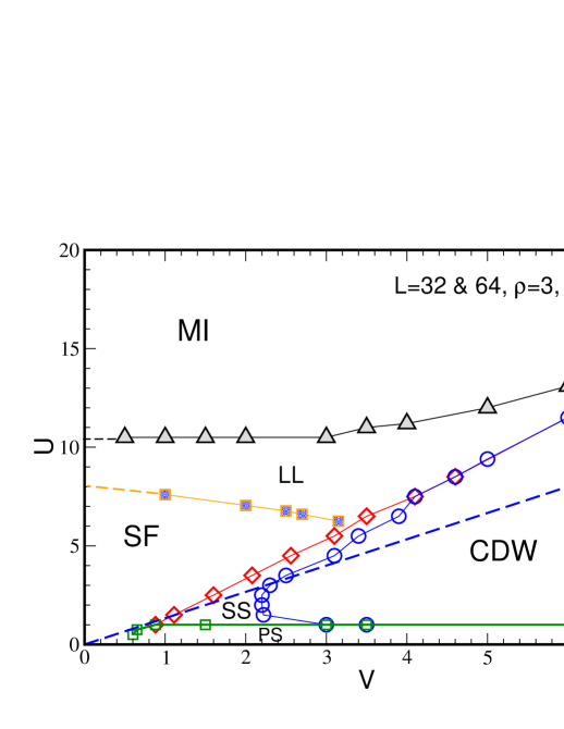
Figure 7: (color online) Applying the same methods as for the $\rho=1$ case, the $\rho=3$ phase diagram is mapped out. Unlike for $\rho=1$, there is no HI here but there is SS. The region of the Luttinger liquid phase (LL) with the Luttinger parameter $K>2$ is indicated by SF and where $K<2$ by LL

The resulting phase diagram at fixed $\rho=1$ is shown in Fig. 6. The open squares are the results of Ref. [rossini12, ], all other symbols are results of our QMC simulations. Our results confirm some of the results of Ref. rossini12, , in particular where their error bars are small, and improve them where their error bars are large. In addition, we have determined the SF-HI boundary and also show the newly found phase separation region. The dashed line is given by $U=4V/3$ and will be discussed below.

Applying the same techniques at fixed filling $\rho=3$ gives the phase diagram Fig. 7. As for the case of $\rho=1$, Fig. 6, the $\rho=3$ phase diagram, Fig. 7, exhibits MI, SF, CDW phases and phase separation. However, it does not exhibit the HI phase. Instead, sandwiched deep between the CDW and MI phases, is a Luttinger liquid (LL) phase with $\langle a^{\phantom{\dagger}}_{0}a^{\dagger}_{r}\rangle\sim r^{-1/2K}$ and parameter $K<2$ and is, therefore, not SF. In addition, the $\rho=3$ phase diagram exhibits a supersolid phase not present at $\rho=1$. The absence of the HI at $\rho=3$ is likely due to the fact that here, unlike for $\rho=1$, the bosonic system cannot be simply mapped on to a Heisenberg spin chain system.

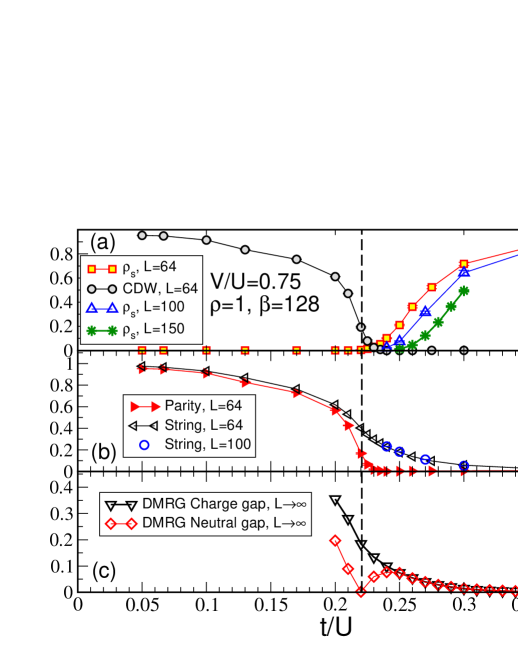
Figure 8: (color online) Shows several quantities for $\rho=1$ as functions of $t/U$ with the fixed ratio $V/U=0.75$. (a) The CDW order parameter for $L=64$ and $\rho_{s}$ for $L=64,\,100,\,150$; (b) the parity and string order parameters; (c) the neutral and charge gaps. (a) and (b) were obtained with QMC and (c) with DMRG. The region to the right of the dashed line is the HI. It terminates at $t/U=0.55$. In the HI, $\rho_{s}\to 0$ very slowly as $L$ increases. Note the difference between the neutral and charge gaps. The gaps are given in units of the hopping $t$.

IV Phase diagram at fixed $V/U=3/4$

In this section we study the phase diagram in the ($\mu/U,t/U$) plane at fixed ratio $V/U=3/4$. This value of $V/U$ is chosen because the CDW phase is favored over the MI phase at large $U$ and integer fillingbatrouni13 .

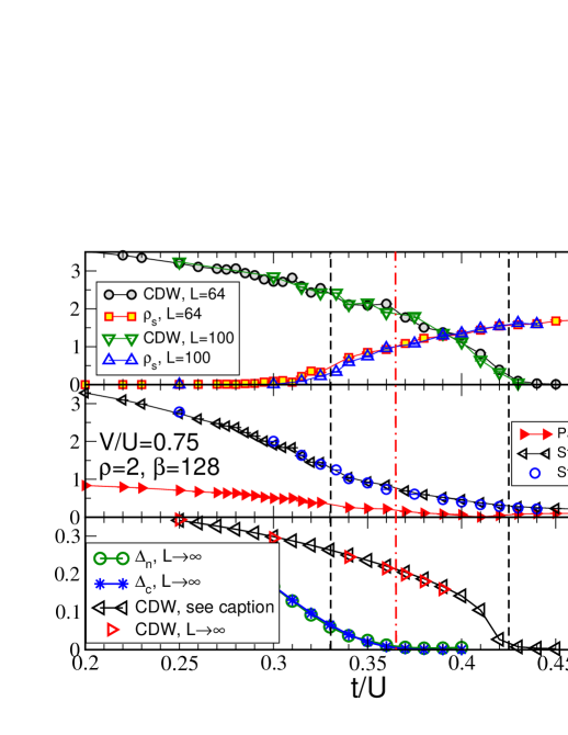
Figure 9: (color online) Same as for $\rho=1$ but at $\rho=2$. (a) QMC simulations show that in the interval between the two vertical (black) dashed lines there is simultaneous SF and CDW order and, therefore, a supersolid phase (SS). The vertical (red) dot-dash line is where the $L\to\infty$ extrapolated neutral ($\Delta_{n}$) and charge ($\Delta_{c}$) gaps vanish in DMRG (c). The CDW-SS transition is between $t/U=0.33$ (QMC) and $t/U=0.355$ (DMRG). The difference between the two values could be due to the difference in the boundary conditions, open for DMRG and periodic for QMC. (c) also shows the $L\to\infty$ extrapolated CDW order parameter, right (red) triangles, and the Fourier transform of $\langle n_{i}\rangle\langle n_{j}\rangle$, left (black) triangles, obtained with DMRG to probe the disappearance of CDW order. Both DMRG and QMC give the SS-SF transition at $t/U\approx 0.425$. Note that, unlike Fig. 8, the charge and neutral gaps (c) are essentially always the same.

We start by fixing $\rho=1$ and studying the various phases as $t/U$ is changed (with $V/U=3/4$). This path is shown as the dashed straight line in Figs. 6 ($\rho=1$) and 7 ($\rho=3$). Figure 8 shows the behavior of $\rho_{s}$, $S(k=\pi)$, ${\cal O}_{s}$, ${\cal O}_{p}$, $\Delta_{c}$ and $\Delta_{n}$ as $t/U$ is changed. For $t/U<0.23$, $\rho_{s}=0$ and $S(\pi)\neq 0$ (Fig. 8(a)) indicating that the system is in the CDW phase. Also in the CDW phase ($t/U<0.23$) ${\cal O}_{p}\neq 0$ and ${\cal O}_{s}\neq 0$ and are both essentially equal to the CDW order parameter, $S(\pi)$. As the transition out of the CDW phase is approached, $t/U\to 0.23$, ${\cal O}_{p}\to 0$ as does $S(\pi)$. However, ${\cal O}_{s}$ decreases but remains finite indicating that the phase is HI for $t/U>0.23$. This scenario is confirmed in Fig. 8(c) which shows the neutral and charge gaps, $\Delta_{n}$ and $\Delta_{c}$. In this panel we see that in the CDW phase, $\Delta_{c}>\Delta_{n}$ and $\Delta_{n}\to 0$ as $t/U\to 0.23$ while $\Delta_{c}$ remains nonzero. In other words, the neutral gap vanishes at the CDW-HI transition but the charge gap remains nonzero showing the HI phase to be gapped. As $t/U$ is increased further, the system eventually transitions into the SF phase which is indicated by the star symbol on the dashed straight line in Fig. 6.

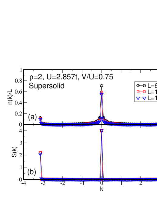
Figure 10: (color online) The dependence of the momentum distribution, $n_{k}/L$, and the structure factor, $S(k)$, on the system size. $n_{k}/L\to 0$ with increasing $L$ while $S(k)$ remains constant indicating long range CDW order.

As mentioned previously, the behavior at $\rho=1$ may be understood by drawing on the analogy with the $S=1$ spin system. The question then arises as to whether the same analogy holds for the other integer fillings. To answer this question we perform the same analysis but for $\rho=2$. The results are shown in Fig. 9. Figure 9(a) shows that for $t/U>0.33$, $\rho_{s}$ increases from zero but $S(\pi)$ remains nonzero. $S(\pi)$ vanishes for $t/U>0.42$ (confirmed by DMRG in panel (c) of the same figure). In other words, unlike the $\rho=1$ case, there is an interval where the system exhibits simultaneous long range diagonal (density) order and superfluidity. This is the hallmark of the SS phase. In the $\rho=1$ case, the HI intervenes between the CDW and SF phases while at $\rho=2$ the SS phase takes that role. To confirm the nature of the SS phase, we show in Fig. 10 the structure factor, $S(k)$ and the momentum distribution, $n(k)$, for several lattice sizes. The fact that the peak $S(\pi)$ does not change with the system size indicates that true long range order in the density is present. The fact that the peak at $n(k=0)$ decreases as $L$ increases is expected since there cannot be true off diagonal long range order in one dimension.

The behavior of the single particle Green function in the SS phase is clarified in Fig. 11 which shows $G(x)$ for $\rho=2$ in the SF, SS and CDW phases. The QMC is done with periodic boundary conditions and consequently, the Green function will be symmetric with respect to $r=L/2$. To handle this, we plot in the figure, on semi-log scale, the Green function versus $x=(L/\pi){\rm sin}(\pi r/L)$ whose limit as $L\to\infty$ is $x=r$. It is seen that in the SF and SS phases, $G(x)$ decays as a power ($K=2.5$ and $K=1.2$ respectively) although in the SS phase there are modulations due to the long range density order. In the CDW phase, $G(x)$ decays exponentially as expected.

The same behavior is observed for $\rho=3$ and, in fact, for $\rho=5/2$. For the $\rho=3/2$ case, it appears that the system exits the CDW phase directly into the SF phase (see below).

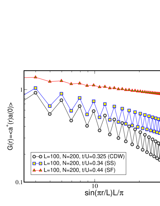
Figure 11: (color online) The single particle Green function decays as a power law in the SF ($K=2.5$) and SS ($K=1.2$) phases and exponentially in the CDW phase. In the SS phase, $G(r)$ also also exhibits oscillations due to the long range density order.

To map out the phase diagram in the ($\mu/U,t/U$) plane we need to characterize the phases at incommensurate fillings. In the top panel of Fig. 12, we show $\rho_{s}$ and $S(\pi)$ as functions of $t/U$ at a filling of $\rho=1.25$ and $V/U=3/4$. We see that two phases are present: SS, where CDW and SF are present simultaneously, and SF.

So, for fixed $V/U=3/4$, we have shown the presence of four phases: CDW, HI, SS and SF. By performing scans such as those that led to Figs. 8, 9, 12 and by calculating the charge gaps for the CDW phase, we find the boundaries of these phases and map the phase diagram in the ($\mu/U,t/U$) plane. The phase diagram is shown in Fig. 13. In Fig. 13, all symbols represent results from QMC simulations for $L=128$ (stars) and $L=64$ (all other symbols), $\beta=128$. The solid black lines near the lobe tips are obtained from DMRG with $L=192$. The end points of the lobes are obtained by studying the finite size dependence of $\Delta_{n}$ using DMRG except for $\rho=1$ which is obtained using QMC by extrapolating ${\cal O}_{s}$ to the thermodynamic limit (the star symbol in Fig. 6). The inset is a zoom of the tip of the $\rho=1$ lobe.

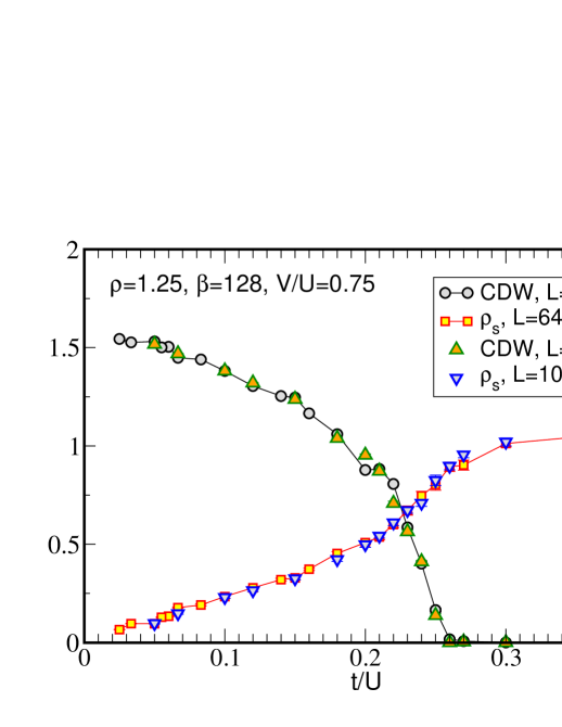
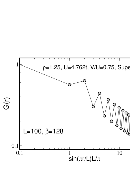
Figure 12: (color online) Top: The superfluid density and the CDW order parameter as functions of $t/U$ at $\rho=1.25$. The system passes from the supersolid phase to the superfluid phase as $t/U$ is increased. Bottom: The one-particle $G(r)$ decays as a power in the SS phase with $K\approx 1.1$.

Several comments are in order. Except for a small region of SS squeezed between it and the $\rho=1$ lobe, the $\rho=1/2$ lobe is surrounded almost entirely by LL phase with $K<2$ and, therefore, not SF, see Fig. 14. The fact that in the extended BHM a SS does not exist when the $\rho=1/2$ CDW phase is doped with holes, but does when it is doped with particles, was already addressed in Ref. [batrouni06, ]. The $\rho=1$ lobe sticks out of the SS phase and the part sticking out is, in fact, the HI phase. No other CDW lobe behaves this way. The $\rho=3/2$ lobe terminates right at the boundary with the SF phase: To within the resolution of our simulations, the transition from the $\rho=3/2$ CDW lobe goes directly into the SF phase without passing through the SS phase. This peculiar behavior for $\rho=3/2$ was also observed with additional DMRG results for different values of $V/U$ ranging from $0.65$ to $1$: The SS layer between the CDW and SF phases, if present, is too thin to observe for the considered system sizes. An accurate determination of the $(U,V)$ phase diagram for this filling will require a more thorough finite size scaling analysis. All other CDW lobes, $\rho\geq 2$, are surrounded entirely by the SS phase. It is interesting to compare this figure with Fig. 3 of Ref. [kawashima12a, ] and with the mean-field predictions Iskin .

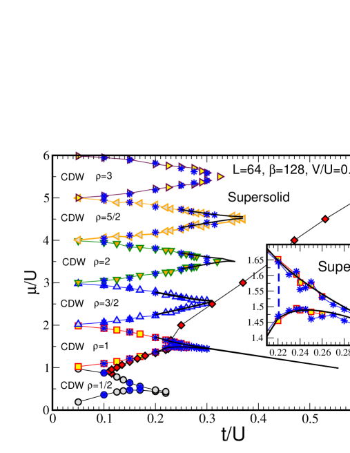
Figure 13: (color online) The phase diagram at fixed ratio $V/U=3/4$. The inset is a zoom on the tip of the $\rho=1$ lobe. All symbols represent results from QMC simulations for $L=128$ (stars) and $L=64$ (all other symbols). The solid black lines near the lobe tips are DMRG results with $L=192$. The end points of the lobes are obtained by studying the finite size dependence of $\Delta_{n}$ using DMRG except for $\rho=1$ which is obtained using QMC by extrapolating ${\cal O}_{s}$ to the thermodynamic limit.

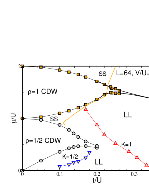
Figure 14: (color online) Detail of the $\rho=1/2$ lobe where we also determined the constant $K$ lines for $K=1,\,1/2$. The Luttinger liquid in this region ($K<2$) is not SF.

V Conclusions

Even though the one dimensional BHM with near neighbor interaction is a rather simple model, it continues to attract attention and to yield surprises such as new phases with exotic order parameters and quantum phase transition.

In this paper we used the SGF QMC algorithm and DMRG to elaborate the details of the phase diagram of the extended BHM in one dimension and expose novel features and exotic phases. We mapped the phase diagrams in the $(\mu/U,t/U)$ plane at fixed $V/U=3/4$ and in the $(U,V)$ plane at two fixed commensurate fillings, $\rho=1,3$. We find that, for this system, the HI seems to exist only at $\rho=1$, invalidating the Heisenberg spin analogy at higher integer fillings. We study the charge and neutral gaps and the nonlocal string order parameter characterizing this phase. For higher densities, we find that the supersolid phase, SS, is very robust and exists for a very wide range of parameters including at commensurate fillings. We show that the one-body Green function decays as a power in the SS phase, not exponentially as sometimes argued. We also showed that when the filling is fixed, there exists a region in the $(U,V)$ plane where the system undergoes phase separation. This phase separated region can be mistaken for a supersolid phase if only the order parameters $\rho_{s}$ and $S(\pi)$ are studied. Evaluation of $\rho(\mu)$ and also the spatial density profile reveals the phase separation unambiguously.

- (1) M.P.A. Fisher, P. B. Weichman, G. Grinstein and D. S. Fisher, Phys. Rev. B40, 546 (1989).
- (2) G. T. Zimanyi, P. A. Crowell, R. T. Scalettar, G. G. Batrouni, Phys. Rev. B50, 6515 (1994).
- (3) M. Greiner, O. Mandel, T. Esslinger, T. W. Hänsch and I. Bloch, Nature 415, 39 (2002).
- (4) D. Jaksch, H.-J. Briegel, J. I. Cirac, C. W. Gardiner and P. Zoller, Phys. Rev. Lett. 82, 1975 (1999).
- (5) G. G. Batrouni, R. T. Scalettar, G. T. Zimanyi and A. P. Kampf, Phys. Rev. Lett. 74, 2527 (1995).
- (6) G. G. Batrouni and R. T. Scalettar, Phys. Rev. Lett. 84, 1599 (2000).
- (7) K. Gral, L. Santos and M. Lewenstein, Phys. Rev. Lett. 88, 170406 (2002).
- (8) S. Wessel and M. Troyer, Phys. Rev. Lett. 95, 127205 (2005).
- (9) M. Boninsegni and N. Prokof’ev, Phys. Rev. Lett. 95, 237204 (2005).
- (10) P. Sengupta, L. P. Pryadko, F. Alet, M. Troyer and G. Schmid, Phys. Rev. Lett. 94, 207202 (2006).
- (11) A. van Otterlo, K-H. Wagenblast, R. Baltin, C. Bruder, R. Fazio and G. Schön, Phys. Rev. B52, 16176 (2005).
- (12) G.G. Batrouni, F. Hébert and R.T. Scalettar, Phys. Rev. Lett. 97, 087209 (2006).
- (13) S. Yi, T. Li and C. P. Sun, Phys. Rev. Lett. 98, 260405 (2007).
- (14) T. Suzuki and N. Kawashima, Phys. Rev. B75, 180502(R) (2007).
- (15) L. Dang, M. Boninsegni and L. Pollet, Phys. Rev. B78, 132512 (2008).
- (16) L. Pollet, J. D. Picon, H. P. Büchler and M. Troyer, Phys. Rev. Lett. 104, 125302 (2010).
- (17) B. Capogrosso-Sansone, C. Trefzger, M. Lewenstein, P. Zoller and G. Pupillo, Phys. Rev. Lett. 104, 125301 (2010).
- (18) F. D. M. Haldane, Phys. Lett. 93A, 464 (1983); Phys. Rev. Lett. 50, 1153 (1983).
- (19) M. den Nijs and K. Rommelse, Phys. Rev. B40, 4709 (1989).
- (20) E. G. Dalla Torre, E. Berg and E. Altman, Phys. Rev. Lett. 97, 260401 (2006).
- (21) E. Berg, E. G. Dalla Torre, T. Giamarchi and E. Altman, Phys. Rev. B77, 245119 (2008).
- (22) P. Niyaz, R. T. Scalettar, C. Y. Fong and G. G. Batrouni, Phys. Rev. B44, 7143(R) (1991).
- (23) P. Niyaz, R. T. Scalettar, C. Y. Fong and G. G. Batrouni, Phys. Rev. B50, 362 (1994).
- (24) T.D. Kühner, S.R. White and H. Monien, Phys. Rev. B61, 12474 (2000).
- (25) D. Rossini and R. Fazio, New J. Phys. 14, 065012 (2012).
- (26) X. Deng, R. Citro, E. Orignac, A. Minguzzi and L. Santos, New Journal of Physics 15 045023 (2013).
- (27) X. Deng and L. Santos, Phys. Rev. B84, 085138 (2011).
- (28) T. Ohgoe, T. Suzuki and N. Kawashima, Phys. Rev. B86, 054520 (2012).
- (29) T. Ohgoe, T. Suzuki and N. Kawashima, Phys. Rev. Lett. 108, 185302 (2012).
- (30) T. Giamarchi, Quantum Physics in One Dimension, (Oxford Science Publications, 2004).
- (31) P. Sengupta and C.D. Batista, Phys. Rev. Lett. 99, 217205 (2007).
- (32) A. Rod, Master thesis, Université de Genève, Switzerland.
- (33) A. Lazarides, O. Tieleman and C. Morais Smith, Phys. Rev. A84, 023620 (2011).
- (34) Yu-Wen Lee, Yu-Li Lee and Min-Fong Yang, Phys. Rev. B76, 075117 (2007).
- (35) G.G. Batrouni, R.T. Scalettar, V. G. Rousseau and B. Grémaud, Phys. Rev. Lett. 110, 265303 (2013).
- (36) V.G. Rousseau, Phys. Rev. E77, 056705 (2008); ibid. E78, 056707 (2008); V.G. Rousseau and D. Galanakis, arXiv:1209.0946.
- (37) B. Bauer et al. (ALPS collaboration), J. Stat. Mech. P05001 (2011).
- (38) L. Barbiero, A. Montorsi, and M. Roncaglia, Phys. Rev. B88, 035109 (2013).
- (39) V. G. Rousseau, arXiv:1403.5472.
- (40) E.L. Pollock and D.M. Ceperley, Phys. Rev. B30, 2555 (1984); D.M. Ceperley and E.L. Pollock, Phys. Rev. Lett. 56, 351 (1986); and E.L. Pollock and D.M. Ceperley, Phys. Rev. Lett. B36, 8343 (1987).
- (41) S. Qin, J. Lou, L. Sun and C. Chen, Phys. Rev. Lett. 90, 067202 (2003).
- (42) M. Oshikawa, J. Phys.: Condens. Matter 4, 7469 (1992); F. Pollmann, E. Berg, A. M. Turner and M. Oshikawa, Phys. Rev. B85, 075125 (2012).
- (43) M. Iskin, Phys. Rev. A83, 051606(R) (2011).