The ROMES method for statistical modeling of reduced-order-model error

Abstract.

This work presents a technique for statistically modeling errors introduced by reduced-order models. The method employs Gaussian-process regression to construct a mapping from a small number of computationally inexpensive ‘error indicators’ to a distribution over the true error. The variance of this distribution can be interpreted as the (epistemic) uncertainty introduced by the reduced-order model. To model normed errors, the method employs existing rigorous error bounds and residual norms as indicators; numerical experiments show that the method leads to a near-optimal expected effectivity in contrast to typical error bounds. To model errors in general outputs, the method uses dual-weighted residuals—which are amenable to uncertainty control—as indicators. Experiments illustrate that correcting the reduced-order-model output with this surrogate can improve prediction accuracy by an order of magnitude; this contrasts with existing ‘multifidelity correction’ approaches, which often fail for reduced-order models and suffer from the curse of dimensionality. The proposed error surrogates also lead to a notion of ‘probabilistic rigor’, i.e., the surrogate bounds the error with specified probability.

1. Introduction

As computing power increases, computational models of engineered systems are being employed to answer increasingly complex questions that guide decision making, often in time-critical scenarios. It is becoming essential to rigorously quantify and account for both aleatory and epistemic uncertainties in these analyses. Typically, the high-fidelity computational model can be viewed as providing a (costly-to-evaluate) mapping between system inputs (e.g., uncertain parameters, decision variables) and system outputs (e.g., outcomes, measurable quantities). For example, data assimilation employs collected sensor data (outputs) to update the distribution of uncertain parameters (inputs) of the model; doing so via Bayesian inference requires sampling from the posterior distribution, which can entail thousands of forward model simulations. The computational resources (e.g., weeks on a supercomputer) required for large-scale simulations preclude such high-fidelity models from being feasibly deployed in such scenarios.

To avoid this bottleneck, analysts have turned to surrogate models that approximate the input–output map of the high-fidelity model, yet incur a fraction of their computational cost. However, to be rigorously incorporated in uncertainty-quantification (UQ) contexts, it is critical to quantify the additional uncertainty introduced by such an approximation. For example, Bayesian inference aims to sample from the posterior distribution

(1) $$\mathrm{P}[{{\bm{\mu}}}|\bar{s}]\propto\mathrm{P}[{{\bm{\mu}}}]\mathrm{P}[\bar{s}|{{\bm{\mu}}}],$$

where ${\bm{\mu}}\in{\mathcal{P}}\subset\mathbb{R}^{n_{{{\bm{\mu}}}}}$ denote system inputs, $\bar{s}\in\mathbb{R}$ denotes the measured output, $\mathrm{P}[{{\bm{\mu}}}]$ represents the prior, and $\mathrm{P}[\bar{s}|{{\bm{\mu}}}]$ denotes the likelihood function. Typically, the measured output is modeled as $\bar{s}=s({{\bm{\mu}}})+\varepsilon$, where $s:{\mathcal{P}}\rightarrow\mathbb{R}$ denotes the outputs predicted by the high-fidelity model for inputs ${{\bm{\mu}}}$, and $\varepsilon$ is a random variable representing measurement noise. Sampling from this posterior distribution (e.g., via Markov-chain Monte–Carlo or importance sampling) is costly, as each sample requires at least one evaluation of the high-fidelity input–output map ${{\bm{\mu}}}\mapsto s$ that appears in the likelihood function.

When a surrogate model is employed, the measured output becomes $\bar{s}=s_{\mathrm{surr}}({{\bm{\mu}}})+\delta_{s}({{\bm{\mu}}})+\varepsilon$, where $s_{\mathrm{surr}}:{\mathcal{P}}\rightarrow\mathbb{R}$ denotes the output predicted by the surrogate model, and $\delta_{s}:{\mathcal{P}}\rightarrow\mathbb{R}$ represents the surrogate-model output error or bias. In this case, posterior sampling requires only evaluations of the surrogate-model input–output map ${{\bm{\mu}}}\mapsto s_{\mathrm{surr}}$—which is computationally inexpensive—as well as evaluation of the surrogate-model error $\delta_{s}({{\bm{\mu}}})$, which is not precisely known in practice. As such, it can be considered a source of epistemic uncertainty, as it can be reduced in principle by employing the original high-fidelity model (or a higher fidelity surrogate model). The goal of this work is to construct a statistical model of this surrogate-model error $\widetilde{\delta_{s}}({{\bm{\mu}}})$ that is 1) cheaply computable, 2) exhibits low variance (i.e., introduces minimal epistemic uncertainty), and 3) whose distribution can be numerically validated.

Various approaches have been developed for different surrogate models to quantify the surrogate error $\delta_{s}({{\bm{\mu}}})$. Surrogate models can be placed into three categories [19]: 1) data fits, 2) lower-fidelity models, and 3) reduced-order models. Data fits employ supervised machine-learning methods (e.g., Gaussian processes, polynomial interpolation [21]) to directly model the high-fidelity input–output map. Within this class of surrogates, it is possible to statistically model the error for stochastic-process data fits, as a prediction for inputs ${{\bm{\mu}}}$ yields a mean $s_{\mathrm{surr}}({{\bm{\mu}}})$ and a mean-zero distribution $\delta_{s}({{\bm{\mu}}})$ that can be associated with epistemic uncertainty. While such models are (unbeatably) fast to query and non-intrusive to implement, they suffer from the curse of dimensionality and lack access to the underlying model’s physics, which can hinder predictive robustness.

Lower-fidelity models simply replace the high-fidelity model with a ‘coarsened’ model obtained by neglecting physics, coarsening the mesh, or employing lower-order finite elements, for example. While such models remain physics based, they often realize only modest computational savings. For such problems, ‘multifidelity correction’ methods have been developed, primarily in the optimization context. These techniques model the mapping ${{\bm{\mu}}}\mapsto\delta_{s}$ using a data-fit surrogate; they either enforce ‘global’ zeroth-order consistency between the corrected surrogate prediction and the high-fidelity prediction at training points [23, 29, 33, 39, 35], or ‘local’ first- or second-order consistency at trust-region centers [2, 19]. Such approaches tend to work well when the surrogate-model error exhibits a lower variance than the high-fidelity response [35] and the input-space dimension is small.

Reduced-order models (ROMs) employ a projection process to reduce the state-space dimensionality of the high-fidelity computational model. Although intrusive to implement, such physics-based surrogates often lead to more significant computational gains than lower-fidelity models, and higher robustness than data fits. For such models, error analysis has been limited primarily to computing rigorous a posteriori error bounds $\Delta_{s}({\bm{\mu}})$ satisfying $\left|\delta_{s}{({\bm{\mu}})}\right|\leq\Delta_{s}({\bm{\mu}})$ [10, 26, 42]. Especially for nonlinear problems, however, these error bounds are often highly ineffective, i.e., they overestimate the actual error by orders of magnitude [17]. To overcome this shortcoming and obtain tighter bounds, the ROM must be equipped with complex machinery that both increases the computational burden [47, 30] and is intrusive to implement (e.g., reformulate the discretization of the high-fidelity model [45, 48]). Further, rigorous bounds are not directly useful for uncertainty quantification (UQ) problems, where a statistical error model that is unbiased, has low variance, and is stochastic is more useful. Recent work [35, Section IV.D] has applied multifidelity correction to ROMs. However, the method did not succeed because the ROM error is often a highly oscillatory function of the inputs and therefore typically exhibits a higher variance than the high-fidelity response.

* probabilistically rigorous
$\dagger$ good effectivity can only be obtained with very intrusive methods.

Table 1. Features of different surrogate models

In this paper, we introduce the ROM Error Surrogates (ROMES) method that aims to combine the utility of multifidelity correction with the computational efficiency and robustness of reduced-order modeling. Table 1 compares the proposed approach with existing surrogate-modeling techniques. Similar to the multifidelity-correction approach, we aim to model the ROM error $\delta_{s}$ using a data-fit surrogate. However, as directly approximating the mapping ${{\bm{\mu}}}\mapsto\delta_{s}$ is ineffective for ROMs, we instead exploit the following key observation: ROMs often generate a small number of physics-based, cheaply computable error indicators $\bm{\rho}:{\mathcal{P}}\rightarrow\mathbb{R}^{q}$ that correlate strongly with the true error $\delta_{s}({\bm{\mu}})$. Examples of indicators include the residual norm, dual-weighted residuals, and the rigorous error bounds discussed above. To this end, ROMES approximates the low-dimensional, well-behaved mapping $\bm{\rho}({\bm{\mu}})\mapsto\delta_{s}({\bm{\mu}})$ using Gaussian-process regression, which is a stochastic-process data-fit method. Note that ROMES constitutes a generalization of the multifidelity correction approach, as the inputs (or features) of the error model can be any user-defined error indicator—they need not be the system inputs ${\bm{\mu}}$. Figure 1 depicts the propagation of information for the proposed method.

In addition to constructing an error surrogate for the system outputs, ROMES can also be used to construct a statistical model for the norm of the error in the system state. Further, ROMES can be used to generate error bounds with ‘probabilistic rigor’, i.e., an error bound that overestimates the error with a specified probability.

Figure 1. ROMES method. The output quantities of interest can be ‘corrected’ by adding the ROM error surrogate to the ROM output prediction, i.e., $s({\bm{\mu}})\approx s_{\text{corr}}({\bm{\mu}})\vcentcolon=s_{\text{red}}({\bm{\mu}})+\widetilde{\delta_{s}}(\bm{\rho}({\bm{\mu}}))$.

Next, Section 2 introduces the problem formulation and provides a general but brief introduction to model reduction. In Section 3, we introduce the ROMES method, including its objectives, ingredients, and some choices of these ingredients for particular errors. Section 4 briefly summarizes the Gaussian-process kernel method [41] and the relevance vector machine [44], which are the two machine-learning algorithms we employ to construct the ROMES surrogates. However, the ROMES methodology does not rely on these two techniques, as any supervised machine learning algorithm that generates a stochastic process can be used, as long as it generates a statistical model that meets the important conditions described in Section 3.1. Section 5 analyses the performance of the method when applied with the reduced-basis method to solve Poisson’s equation in two dimensions using nine system inputs. The method is also compared with existing rigorous error bounds for normed errors, and with the multifidelity correction approach for errors in general system outputs.

For additional information on the reduced-basis method, including the algorithms to generate the reduced-basis spaces and the computation of error bounds, we refer to the supplementary Section A.

2. Problem formulation

This section details aspects of the high-fidelity and reduced-order models that are important for the ROMES surrogates. We begin with a formulation of the high-fidelity model in Section 2.1 and the reduced-order model in Section 2.2. Finally, we elaborate on the errors introduced by the model-reduction process and possible problems with their quantification in Section 2.3.

2.1. High-fidelity model

Consider solving a parameterized systems of equations

(2) $$\bm{r}({\bm{u}};{{{\bm{\mu}}}})=0,$$

where ${\bm{u}}:{\mathcal{P}}\rightarrow\mathbb{R}^{n}$ denotes the state implicitly defined by Eq. (2), ${{{\bm{\mu}}}}\in{\mathcal{P}}\subset\mathbb{R}^{{n_{{{\bm{\mu}}}}}}$ denotes the system inputs, and $\bm{r}:\mathbb{R}^{n}\times\mathbb{R}^{{n_{{{\bm{\mu}}}}}}\rightarrow\mathbb{R}^{n}$ denotes the residual operator. This model is appropriate for stationary problems, e.g., those arising from the finite-element discretization of elliptic PDEs. For simplicity, assume we are interested in computing a single output

(3) $$s({{{\bm{\mu}}}})\vcentcolon=g({\bm{u}}({{{\bm{\mu}}}}))$$

with $s:\mathbb{R}^{{n_{{{\bm{\mu}}}}}}\rightarrow\mathbb{R}$ and $g:\mathbb{R}^{n}\rightarrow\mathbb{R}$.

When the dimension $n$ of the high-fidelity model is ‘large’, computing the system outputs $s$ by first solving Eq. (2) and subsequently applying Eq. (3) can be prohibitively expensive. This is particularly true for many-query problems arising in UQ such as Bayesian inference, which may require thousands of input–output map evaluations ${{{\bm{\mu}}}}\mapsto s$.

2.2. Reduced-order model

Model-reduction techniques aim to reduce the burden of solving Eq. (2) by employing a projection process. First, they execute a computationally expensive offline stage (e.g., solving Eq. (2) for a training set ${{{\bm{\mu}}}}\in{\mathcal{P}}_{\mathrm{train}}\subset{\mathcal{P}}$) to construct 1) a low-dimensional trial basis (in matrix form) $\bm{V}\in\mathbb{R}^{n\times p}$ with $p\ll n$ that (hopefully) captures the behavior of the state ${\bm{u}}$ throughout the parameter domain ${\mathcal{P}}$, and 2) an associated test basis $\bm{W}\in\mathbb{R}^{n\times p}$. Then, during the computationally inexpensive online stage, these methods approximately solve Eq. (2) for arbitrary ${{{\bm{\mu}}}}\in{\mathcal{P}}$ by searching for solutions in the trial subspace $\mathrm{range}\left(\bm{V}\right)\subset\mathbb{R}^{n}$ and enforcing orthogonality of the residual $\bm{r}$ to the test subspace $\mathrm{range}\left(\bm{W}\right)\subset\mathbb{R}^{n}$:

(4) $$\bm{W}^{t}\bm{r}(\bm{V}\hat{\bm{u}};{{{\bm{\mu}}}})=0.$$

Here, the state is approximated as ${\bm{u}}_{\text{red}}({{{\bm{\mu}}}})\vcentcolon=\bm{V}\hat{\bm{u}}({{{\bm{\mu}}}})$ and the reduced state $\hat{\bm{u}}({{{\bm{\mu}}}})\in\mathbb{R}^{p}$ is implicitly defined by Eq. (4). The ROM-predicted output is then $s_{\text{red}}({\bm{\mu}})\vcentcolon=g\left({\bm{u}}_{\text{red}}({{{\bm{\mu}}}});{{{\bm{\mu}}}}\right)$.

When the residual operator is nonlinear in the state or non-affine in the inputs, additional complexity-reduction approximations such as empirical interpolation [5, 24], collocation [31, 3, 43], discrete empirical interpolation [15, 22, 18], or gappy proper orthogonal decomposition (POD) [13, 14] are required to ensure that computing the low-dimensional residual $\bm{W}^{t}\bm{r}$ incurs an $n$-independent operation count. In this case, the residual is approximated as $\tilde{}\bm{r}\approx\bm{r}$ and the reduced-order equations become

(5) $$\bm{W}^{t}\tilde{}\bm{r}(\bm{V}\hat{\bm{u}};{{{\bm{\mu}}}})=0.$$

When the output operator is nonlinear and the vector $\partial g/\partial{\bm{u}}$ is dense, approximations in the output calculation are also required to ensure an $n$-independent operation count.

Section A describes in detail the construction of a reduced-order model using the reduced-basis method applied to a parametrically coercive, affine, linear, elliptic PDE.

2.3. Reduced-order-model error bounds

One is typically interested in quantifying two types of error incurred by model reduction: the state-space error ${\bm{\delta}_{{\bm{u}}}}({{{\bm{\mu}}}})\vcentcolon={\bm{u}}({{{\bm{\mu}}}})-{\bm{u}}_{\text{red}}({{{\bm{\mu}}}})\in\mathbb{R}^{n}$ and the output error $\delta_{s}{({\bm{\mu}})}\vcentcolon=s({\bm{\mu}})-s_{\text{red}}({\bm{\mu}})\in\mathbb{R}{}$. In particular, many ROMs are equipped with computable, rigorous error bounds for these quantities [37, 25, 36, 11, 17]:

(6) $$\Delta_{{\bm{u}}}{({\bm{\mu}})}\geq\left\|{\bm{\delta}_{{\bm{u}}}}({\bm{\mu}})\right\|,\qquad\Delta_{s}{({\bm{\mu}})}\geq\left|\delta_{s}{({\bm{\mu}})}\right|$$

In cases, where the norm of the residual operator can be estimated tightly, lower bounds also exist:

(7) $$\Delta^{\text{LB}}_{{\bm{u}}}{({\bm{\mu}})}\leq\left\|{\bm{\delta}_{{\bm{u}}}}({\bm{\mu}})\right\|,\qquad\Delta^{\text{LB}}_{s}{({\bm{\mu}})}\leq\left|\delta_{s}{({\bm{\mu}})}\right|.$$

The performance of an upper bound is usually quantified by its effectivity, i.e., the factor by which it overestimates the true error

(8) $$\eta^{\bm{u}}({\bm{\mu}})\vcentcolon=\frac{\Delta_{{\bm{u}}}{({\bm{\mu}})}}{\left\|{\bm{\delta}_{{\bm{u}}}}({\bm{\mu}})\right\|}\geq 1,\qquad\eta^{s}({\bm{\mu}})\vcentcolon=\frac{\Delta_{s}{({\bm{\mu}})}}{\left|\delta_{s}{({\bm{\mu}})}\right|}\geq 1.$$

The closer these values are to $1$, the ‘tighter’ the bound. For coercive PDEs, these effectivities can be controlled by choosing a tight lower bound of the coercivity constant.

While this can be easily accomplished for stationary, linear problems, it is difficult to find tight lower bounds in almost all other cases. In fact, the resulting bounds often overestimate the error by orders of magnitude [42, 17]. Because effectivity is critically important in practice, various efforts have been undertaken to improve the tightness of the bounds. Huynh et al. [30] developed the successive constraint method for this purpose; the method approximates the coercivity-constant lower bounds by solving small linear programs online, which depend on additional expensive offline computations. Alternatively, Refs. [45, 48] reformulate the entire discretization of time-dependent problems using a space–time method that improves the error bounds by incorporating solutions to dual problems. Another approach [47] aims to approximate the coercivity constant by eigenvalue analysis of the reduced system matrices. These methods all bloat the offline and the online computation time and often incur intrusive changes to the high-fidelity-model implementation.

Regardless of effectivity, rigorous bounds satisfying inequalities (6) are not directly useful for quantifying the epistemic uncertainty incurred by employing the ROM. Rather, a statistical model that reflects our knowledge of these errors would be more appropriate. For such a model, the mean of the distribution would provide an expected error; the variance would provide a notion of epistemic uncertainty. The most straightforward way to achieve this would be to model the error as a uniform probability distribution on an interval whose boundaries correspond to the lower and upper bounds. Unfortunately, such an approach leads to wide, uninformative intervals when the bounds suffer from poor effectivity; this will be demonstrated in the numerical experiments.

Instead, we exploit the following observation: error bounds tend to be strongly correlated with the true error. Figure 2 depicts this observed structure for a reduced-basis ROM applied to an elliptic PDE (see Section 5.1 for details). On a logarithmic scale, the true error exhibits a roughly linear dependence on both the bound and the residual norm, and the variance of the data is fairly constant. As will be shown in Section 5.3, employing a multifidelity correction approach wherein the error is modeled as a function of the inputs ${{{\bm{\mu}}}}$ does not work well for this example, both because the input-space dimension is large (nine) and the error is a highly oscillatory function of these inputs.

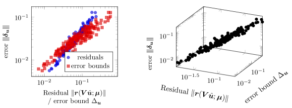
Figure 2. Relationship between RB error bounds $\Delta_{{\bm{u}}}$, residual norms $\|\bm{r}(\bm{V}\hat{\bm{u}};{{{\bm{\mu}}}})\|$, and the true state-space errors ${\left|\kern-1.07639pt\left|\kern-1.07639pt\left|{\bm{\delta}_{{\bm{u}}}}\right|\kern-1.07639pt\right|\kern-1.07639pt\right|}$, visualized by evaluation of $200$ random sample points in the input space. Here, ${\left|\kern-1.07639pt\left|\kern-1.07639pt\left|\cdot\right|\kern-1.07639pt\right|\kern-1.07639pt\right|}$ denotes the energy norm defined in Section 5.1.

Therefore, we propose constructing a stochastic process that maps such error indicators to a random variable for the error. For this purpose, we employ Gaussian-process regression. The approach leverages one strength of ROMs compared to other surrogate models: ROMs generate strong ‘physics-based’ error indicators (e.g., error bounds) in addition to output predictions. The next section describes the proposed method.

3. The ROMES method

The objective of the ROMES method is to construct a statistical model of the deterministic, but generally unknown ROM error $\delta({{{\bm{\mu}}}})$ with $\delta:{\mathcal{P}}\to\mathbb{R}$ denoting an $\mathbb{R}{}$-valued error that may represent the norm of the state-space error $\left\|{\bm{\delta}_{{\bm{u}}}}\right\|$, the output error $\delta_{s}$, or its absolute value $|\delta_{s}|$, for example. The distribution of the random variable representing the error should reflect our (epistemic) uncertainty about its value. We assume that we can employ a set of training points $\delta({{{\bm{\mu}}}}_{n})$, $n=1,\ldots,N$ to construct this model.

3.1. Statistical model

Define a probability space $(\Omega,\mathcal{F},P)$. We seek to approximate the deterministic mapping $m:{{{\bm{\mu}}}}\mapsto d(\delta({{{\bm{\mu}}}}))$ by a stochastic mapping $\tilde{m}:\bm{\rho}({{{\bm{\mu}}}})\mapsto\tilde{d}$ with $\tilde{d}:\Omega\rightarrow\mathbb{R}{}$ a real-valued random variable. Here, $d:\mathbb{R}{}\rightarrow\mathbb{R}{}$ is an invertible transformation function (e.g., logarithm) that can be specified to facilitate construction of the statistical model. We can then interpret the statistical model of the error as a random variable $\tilde{\delta}:\bm{\rho}\mapsto d^{-1}(\tilde{m}(\bm{\rho}))$.

Three ingredients must be selected to construct this mapping $\tilde{m}$: 1) the error indicators $\bm{\rho}$, 2) the transformation function $d$, and 3) the methodology for constructing the statistical model from the training data. We will make these choices such that the stochastic mapping satisfies the following conditions:

1. The indicators $\bm{\rho}({{{\bm{\mu}}}})$ are cheaply computable and low dimensional given any ${{{\bm{\mu}}}}\in{\mathcal{P}}$. In practice, they should also incur a reasonably small implementation effort, e.g., not require modifying the underlying high-fidelity model.

2. The mapping $\tilde{m}$ exhibits low variance, i.e., $\mathrm{E}\left[\left(\tilde{m}(\bm{\rho}({{{\bm{\mu}}}}))-\mathrm{E}\left[\tilde{m}(\bm{\rho}({{{\bm{\mu}}}}))\right]\right)^{2}\right]$ is ‘small’ for all ${{{\bm{\mu}}}}\in{\mathcal{P}}$. This ensures that little additional epistemic uncertainty is introduced.

3. The mapping $\tilde{m}$ is validated:

   (9) $${{\omega}_{\text{validation}}\left({\omega}\right)}\approx{\omega},\quad\forall{\omega}\in\left[0,1\right),$$

   where ${{\omega}_{\text{validation}}\left({\omega}\right)}$ is the frequency with which validation data lie in the ${\omega}$-confidence interval predicted by the statistical model

   (10) $${{\omega}_{\text{validation}}\left({\omega}\right)}\vcentcolon=\frac{\mathrm{card}\left(\{{\bm{\mu}}\in{\mathcal{P}}_{\mathrm{validation}}\ |\ d(\delta({{{\bm{\mu}}}}))\in C_{{\omega}}\left({{{\bm{\mu}}}}\right)\}\right)}{\mathrm{card}\left({\mathcal{P}}_{\mathrm{validation}}\right)}.$$

   Here, the validation set ${\mathcal{P}}_{\mathrm{validation}}\subset{\mathcal{P}}$ should not include any of the points ${{{\bm{\mu}}}}_{n}$, $n=1,\ldots,N$ employed to train the error surrogate, and the confidence interval $C_{{\omega}}\left({{{\bm{\mu}}}}\right)\subset\mathbb{R}{}$, which is centered at the mean of $\tilde{m}(\bm{\rho}({{{\bm{\mu}}}}))$, is defined for all ${{{\bm{\mu}}}}\in{\mathcal{P}}$ such that

   (11) $$\mathrm{P}[\tilde{m}(\bm{\rho}({{{\bm{\mu}}}}))\in{C_{{\omega}}\left({{{\bm{\mu}}}})\right)}]={\omega}.$$

   In essence, validation assesses whether or not the data do indeed behave as random variables with probability distributions predicted by the statistical model.

The next section describes the proposed methodology for selecting indicators $\bm{\rho}$ and transformation function $d$. For constructing the mapping $\tilde{m}$ from training points, we will employ the two supervised machine learning algorithms described in Section 4: the Gaussian process (GP) kernel method and the relevance vector machine (RVM). Note that these are merely guidelines for model construction, as there are usually no strong analytical tools to prove that the mapping behaves according to a certain probability distribution. Therefore, any choice must be computationally validated according to condition 3 above.

3.2. Choosing indicators and transformation function

The class of multifidelity-correction algorithms can be cast within the framework proposed in Section 3.1. In particular, when a stochastic process is used to model additive error, these methods are equivalent to the proposed construction with ingredients $\delta=\delta_{s}$, $\bm{\rho}={{{\bm{\mu}}}}$, and $d=\mathrm{id}_{\mathbb{R}{}}$ with $\mathrm{id}_{\mathbb{R}{}}(x)=x$, $\forall x\in\mathbb{R}{}$ the identity function over $\mathbb{R}{}$. However, as previously discussed, the mapping ${\bm{\mu}}\mapsto\delta_{s}$ can be highly oscillatory and non-smooth for reduced-order models; further, this approach is infeasible for high-dimensional input spaces, i.e., ${n_{{{\bm{\mu}}}}}$ large. This was shown by Ng and Eldred [35, Section IV.D]; we also demonstrate this in the numerical experiments of Section 5.3.

Note that all indicators and errors proposed in this section should be scaled (e.g., via linear transformations) in practice such that they exhibit roughly the same range. This ‘feature scaling’ task is common in machine-learning and is particularly important when the ROMES surrogate employs multiple indicators.

3.2.1. Normed and compliant outputs

As discussed in Section 2.3, many ROMs are equipped with bounds for normed errors. Further, there is often a strong, well-behaved relationship between such error bounds and the normed error (see Figure 2). In the case of compliant outputs, the error is always non-negative, i.e., $\delta_{s}=|\delta_{s}|$ (see Section A.3), so we can treat this error as a normed error.

To this end, we propose employing error bounds as indicators for the errors in the compliant output $|\delta_{s}|$ and in the state $\left\|{\bm{\delta}_{{\bm{u}}}}\right\|$. However, because the bound effectivity often lies in a small range (even for a large range of errors) [42], employing a logarithmic transformation is appropriate. To see this, consider a case where the effectivity $\eta$ of the error bound, defined as

(12) $$\eta({\bm{\mu}})\vcentcolon=\frac{\Delta{({\bm{\mu}})}}{\delta{({\bm{\mu}})}}\geq 1,\quad\forall{\bm{\mu}}\in{\mathcal{P}},$$

lies within a range $\eta_{1}\leq\eta({\bm{\mu}})\leq\eta_{2}$, $\forall{\bm{\mu}}\in{\mathcal{P}}$. Then the relationship between the error bound and the true error is

(13) $$\frac{\Delta{({\bm{\mu}})}}{\eta_{1}}\geq\delta{({\bm{\mu}})}\geq\frac{\Delta{({\bm{\mu}})}}{\eta_{2}}$$

(14) $$\log{\Delta{({\bm{\mu}})}}-\log{\eta_{1}}\geq\log{\delta{({\bm{\mu}})}}\geq\log{\Delta{({\bm{\mu}})}}-\log{\eta_{2}}$$

for all ${\bm{\mu}}\in{\mathcal{P}}$. In this case, one would expect an affine model mapping $\log{\Delta{({\bm{\mu}})}}$ to $\log{\delta{({\bm{\mu}})}}$ with constant Gaussian noise to accurately capture the relationship. So, employing a logarithmic transformation permits the use of simpler surrogates that assume a constant variance in the error variable. Therefore, we propose employing $\bm{\rho}=\log{\Delta}$ and $d=\log$ for statistical modeling of normed errors and compliant outputs.

A less computationally expensive candidate for an indicator is simply the logarithm of the residual norm $\bm{\rho}=\log{{r}}$, where ${r}$ is the Euclidean norm of the residual vector

(15) $${r}({\bm{\mu}})\vcentcolon=\left\|\bm{r}(\bm{V}\hat{\bm{u}}({{{\bm{\mu}}}});{{{\bm{\mu}}}})\right\|_{2}.$$

For more information on the efficient computation of (15), we refer to Section A.3.1. One would expect this choice of indicator to produce a similar model to that produced by the logarithm of the error bound: the error bound is often equal to the residual norm divided by a (costly-to-compute) coercivity-constant lower bound (see Section A.3). Further, employing the residual norm leads to a model that is less sensitive to strong variations in this approximated lower bound.

Returning to the example depicted in Figure 2, the relationship between the error bound and the energy norm of the state error in log-log space is roughly linear, and the variance is relatively small. The same is true of the relationship between the (computationally cheaper) residual norm and the true error. As expected, these relationships can be accurately modeled as a stochastic process with a linear mean function and constant variance (more details in Section 5.1). Here, strong candidates for ROMES error indicators include $\bm{\rho}_{1}({\bm{\mu}})\vcentcolon={r}({\bm{\mu}}),\bm{\rho}_{2}({\bm{\mu}})\vcentcolon=\Delta{({\bm{\mu}})}$, and $\bm{\rho}_{3}({\bm{\mu}})\vcentcolon=\left({r}({\bm{\mu}}),\Delta{({\bm{\mu}})}\right)$. In the experiments in Section 5, we will consider the first choice, which is the least expensive and intrusive option, yet leads to excellent results. For cases where the data are less well behaved, more error indicators can be included, e.g., linear combinations of inputs or the output prediction.

Unfortunately, this set of ROMES ingredients is not applicable to errors in general outputs of interest because the logarithmic transformation function assumes strictly positive errors. The next section presents a strategy for handling this general case.

Remark 3.1 (Log-Normal distribution).

In the case where $d=\log$, the error models $\widetilde{\delta}({\bm{\mu}})$, ${\bm{\mu}}\in{\mathcal{P}}$ are random variables with log-normal distribution. If one is interested in the most probable error, one might think to use the expected value of $\widetilde{\delta{}}$. However, the maximum of the probability distribution function of a log-normally distributed random variable is defined by its mode, which is less than the expected value. We therefore use $\mathrm{mode}(\widetilde{\delta{}})$ if scalar values for the estimation of the output error or the reduced state error are required.

3.2.2. General outputs

This section describes the ROMES ingredients we propose for modeling the error $\delta_{s}$ in a general output $s({{{\bm{\mu}}}})\vcentcolon=g({\bm{u}}({{{\bm{\mu}}}}))$. Dual-weighted-residual approaches are commonly adopted for approximating general output errors in the context of a posteriori adaptivity [20, 4, 7, 40, 46, 32], model-reduction adaptivity [12], and model-reduction error estimation [38, 11, 45, 34]. The latter references compute adjoint solutions in order to improve the accuracy of ROM output-error bounds. The computation of these adjoint solutions entails a low-dimensional linear solve; thus, they are efficiently computable and can potentially serve as error indicators for the ROMES method.

The main idea of dual-weighted-residual error estimation is to approximate the output error to first-order using the solution to a dual problem. For notational simplicity in this section, we drop dependence on the inputs ${{{\bm{\mu}}}}$.

To begin, we approximate the output arising from the (unknown) high-fidelity state ${\bm{u}}$ to first order about the ROM-approximated state $\bm{V}\hat{\bm{u}}$:

(16) $$g\left({\bm{u}}\right)\approx g\left(\bm{V}\hat{\bm{u}}\right)+\frac{\partial g}{\partial{\bm{u}}}\left(\bm{V}\hat{\bm{u}}\right)\left({\bm{u}}-\bm{V}\hat{\bm{u}}\right)$$

with $g:\mathbb{R}^{n}\rightarrow\mathbb{R}{}$ and $\frac{\partial g}{\partial{\bm{u}}}:\mathbb{R}^{n}\rightarrow\mathbb{R}^{1\times n}$. Similarly, we can approximate the residual to first order about the approximated state as

(17) $$0=\bm{r}\left({\bm{u}}\right)\approx\bm{r}\left(\bm{V}\hat{\bm{u}}\right)+\frac{\partial\bm{r}}{\partial{\bm{u}}}\left(\bm{V}\hat{\bm{u}}\right)\left({\bm{u}}-\bm{V}\hat{\bm{u}}\right),$$

where $\bm{r}:\mathbb{R}^{n}\rightarrow\mathbb{R}^{n}$ with $\frac{\partial\bm{r}}{\partial{\bm{u}}}:\mathbb{R}^{n}\rightarrow\mathbb{R}^{n\times n}$. Solving for the error yields

(18) $$\left({\bm{u}}-\bm{V}\hat{\bm{u}}\right)\approx-\left[\frac{\partial\bm{r}}{\partial{\bm{u}}}\left(\bm{V}\hat{\bm{u}}\right)\right]^{-1}\bm{r}\left(\bm{V}\hat{\bm{u}}\right).$$

Substituting (18) in (16) leads to

(19) $$g\left({\bm{u}}\right)-g\left(\bm{V}\hat{\bm{u}}\right)\approx\bm{y}^{T}\bm{r}\left(\bm{V}\hat{\bm{u}}\right),$$

where the dual solution $\bm{y}\in\mathbb{R}^{n}$ satisfies

(20) $$\frac{\partial\bm{r}}{\partial{\bm{u}}}^{t}(\bm{V}\hat{\bm{u}})\bm{y}=-\frac{\partial g}{\partial{\bm{u}}}^{t}\left(\bm{V}\hat{\bm{u}}\right).$$

Approximation (19) is first-order accurate; therefore, it is exact in the case of linear outputs and a linear residual operator. In the general nonlinear case, this approximation is accurate in a neighborhood of the ROM-approximated state $\bm{V}\hat{\bm{u}}$.

Because we would like to avoid high-dimensional solves, we approximate $\bm{y}$ as the reduced-order dual solution $\bm{y}_{\text{red}}\vcentcolon=\bm{Y}\hat{\bm{y}}\in\mathbb{R}^{n}$, where $\hat{\bm{y}}$ satisfies

(21) $$\bm{Y}^{T}\frac{\partial\bm{r}}{\partial{\bm{u}}}^{t}(\bm{V}\hat{\bm{u}})\bm{Y}\hat{\bm{y}}=\bm{Y}^{T}\frac{\partial g}{\partial{\bm{u}}}^{t}\left(\bm{V}\hat{\bm{u}}\right),$$

and $\bm{Y}\in\mathbb{R}^{n\times p_{y}}$ with $p_{y}\ll n$ is a reduced basis (in matrix form) for the dual system. Section A.3.2 provides details on the construction of $\bm{Y}$ for elliptic PDEs. Substituting the approximation $\bm{y}_{\text{red}}$ for $\bm{y}$ in (19) yields a cheaply computable error estimate

(22) $$g\left({\bm{u}}\right)-g\left(\bm{V}\hat{\bm{u}}\right)\approx\bm{y}_{\text{red}}^{t}\bm{r}\left(\bm{V}\hat{\bm{u}}\right).$$

This relationship implies that one can construct an accurate, cheaply computable ROMES model for general-output error $\delta=\delta_{s}=g({\bm{u}})-g(\bm{V}\hat{\bm{u}})$ by employing indicators $\bm{\rho}=\bm{y}_{\text{red}}^{t}\bm{r}\left(\bm{V}\hat{\bm{u}}\right)$ and transformation function $d=\mathrm{id}_{\mathbb{R}{}}$ the identity function over $\mathbb{R}{}$.

Remark 3.2 (Uncertainty control for dual-weighted-residual error indicators).

The accuracy of the reduced-order dual solution can be controlled by changing $p_{y}$—the dimension of the dual basis $\bm{Y}$. In general, one would expect an increase in $p_{y}$ to lead to a lower-variance ROMES surrogate at the expense of a higher dimensional dual problem (21). The experiments in Section 5.6 highlight this uncertainty-control attribute.

3.3. Probabilistically rigorous error bounds

Clearly, the ROMES surrogate does not strictly bound the error, even when error bounds are used as indicators. That is, the mean probability of overestimation is generally less than one

(23) $$c\vcentcolon=\frac{1}{|{\mathcal{P}}|}\int_{{\bm{\mu}}\in{\mathcal{P}}}\mathrm{P}[\tilde{m}(\bm{\rho}({\bm{\mu}}))>d(\delta{({\bm{\mu}})})]d{\bm{\mu}}<1.$$

This frequency of overestimation depends on the probability distribution of the random variable $\tilde{m}(\bm{\rho})$. Using the machine learning methods proposed in the next section, we infer normally distributed random variables

(24) $$\tilde{m}(\bm{\rho})\sim{\mathcal{N}}(\nu(\bm{\rho}),\overline{\sigma}^{2}(\bm{\rho}))$$

with mean $\nu(\bm{\rho})$ and variance $\overline{\sigma}^{2}(\bm{\rho})$. If the model is perfectly validated, then the mean probability of overestimation is $c=0.5$. However, knowledge about the distribution of the random variable can be used to control the overestimation frequency. In particular, the modified surrogate

(25) $${\tilde{m}{}}^{c}(\bm{\rho})\vcentcolon={\tilde{m}{}}(\bm{\rho})+m_{\mathrm{LB}}(\bm{\rho},c)$$

enables probabilistic rigor: it bounds the error with mean specified probability $c$ assuming the model is perfectly validated. Here, $m_{\mathrm{LB}}$ fulfills

(26) $$\mathrm{P}[X>m_{\mathrm{LB}}(\bm{\rho},c)]=c,\qquad\text{ for~{}}X\sim{\mathcal{N}}(0,\overline{\sigma}^{2}(\bm{\rho})).$$

This value can be computed as

(27) $$m_{\mathrm{LB}}(\bm{\rho})=\sqrt{2}\overline{\sigma}(\bm{\rho})\mathrm{erf}^{-1}\left(2c-1\right)$$

where $\mathrm{erf}^{-1}$ is the inverse of the error function.

4. Gaussian processes

This section describes the two methods we employ to construct the stochastic mapping $\tilde{m}:\bm{\rho}({{{\bm{\mu}}}})\mapsto\tilde{d}$:

• Gaussian process kernel regression (i.e., kriging) [41] and

• the relevance vector machine (RVM) [44].

Both methods are examples of supervised learning methods that generate a stochastic process from a set of $N$ training points for independent variables $\mathbf{x}\vcentcolon=(\bm{x}_{n})_{n=1}^{N}$ and a dependent variable $\mathbf{y}\vcentcolon=(y_{n})_{n=1}^{N}$. Using these training data, the methods generate predictions $\tilde{y}(\bm{x}_{m}^{*};\theta^{\text{ML}})$, $m=1,\ldots,M$ associated with a set of $M$ prediction points $\mathbf{x}^{*}\vcentcolon=(\bm{x}^{*}_{m})_{m=1}^{M}$. Here, $\theta^{\text{ML}}$ denotes hyperparameters that are inferred using a Bayesian approach; the predictions are random variables with a multivariate normal distribution.

In the context of ROMES, the independent variables correspond to error indicators $\bm{x}_{n}=\bm{\rho}({{{\bm{\mu}}}}_{n})$ with ${{{\bm{\mu}}}}_{n}\in{\mathcal{P}}$, $n=1,\ldots,N$ and the dependent variable corresponds to the (transformed) reduced-order-model error such that $y_{n}=d(\delta({{{\bm{\mu}}}}_{n}))$, $n=1,\ldots,N$. To make this paper as self-contained as possible, the following sections briefly present and compare the two approaches.

4.1. GP kernel method

A Gaussian process is defined as a collection of random variables such that any finite number of them has a joint Gaussian distribution. The GP kernel method constructs this Gaussian process via Bayesian inference using the training data and a specified kernel function. To begin, the prior distribution is set to

(28) $$\tilde{y}_{\mathrm{prior}}(\underline{\mathbf{x}})\sim\mathcal{N}\left(0,\mathbf{K}\left(\underline{\mathbf{x}},\underline{\mathbf{x}}\right)+\sigma^{2}\mathbf{I}_{N+M}\right)$$

with $\underline{\mathbf{x}}\vcentcolon=\left(\underline{\bm{x}}_{i}\right)_{i=1}^{N+M}=(\mathbf{x},\mathbf{x}^{*})$. Here, the GP kernel assumes that the covariance between any two points can be described analytically by a kernel $k$ with additive noise $\bm{\epsilon}\sim{\mathcal{N}}(0,\sigma^{2}\mathbf{I}_{M+N})$ such that

(29) $$\mathbf{K}(\underline{\mathbf{x}},\underline{\mathbf{x}})=\left(k(\underline{\bm{x}}_{i},\underline{\bm{x}}_{j})\right)_{1\leq i,j\leq N+M}.$$

In this work, we employ the most commonly used squared-exponential-covariance kernel

(30) $$k(\bm{x}_{i},\bm{x}_{j}) =\exp\left(-\frac{\|{\bm{x}_{i}-\bm{x}_{j}}\|_{2}^{2}}{2l^{2}}\right),$$

which induces high correlation between geometrically nearby points. Here, $l\in\mathbb{R}{}$ is the ‘width’ hyperparameter.

Assuming the predictions are generated as independent samples from the stochastic process, the GP kernel method then generates predictions for each point $\bm{x}^{*}\in\mathbf{x}^{*}$. These predictions correspond to random variables with posterior distributions $\tilde{y}(\bm{x}^{*};\theta)\sim{\mathcal{N}}(\nu(\bm{x}^{*}),\overline{\sigma}^{2}(\bm{x}^{*}))$ with

(31) $$\nu(\bm{x}^{*}) =\mathbf{K}(\bm{x}^{*},\mathbf{x})\left(\mathbf{K}(\mathbf{x},\mathbf{x})+\sigma^{2}\mathbf{I}_{N}\right)^{-1}\mathbf{y}$$

(32) $$\overline{\sigma}^{2}(\bm{x}^{*}) =\Sigma(\bm{x}^{*})+\sigma^{2}$$

(33) $$\Sigma(\bm{x}^{*}) =\mathbf{K}(\bm{x}^{*},\bm{x}^{*})-\mathbf{K}(\bm{x}^{*},\mathbf{x})\left(\mathbf{K}(\mathbf{x},\mathbf{x})+\sigma^{2}\mathbf{I}_{N}\right)^{-1}\mathbf{K}(\mathbf{x},\bm{x}^{*}).$$

More details on the derivation of these expressions can be found in Ref. [41, ch 2.2].

The hyperparameters $\theta\vcentcolon=(l^{2},\sigma^{2})$ can be set to the maximum-likelihood values $\theta^{\text{ML}}$ computed as the solution to an optimization problem

(34) $$\theta^{\text{ML}}=\arg\max_{\theta}{\mathcal{L}}(\theta)$$

with the log-likelihood function defined as

(35) $${\mathcal{L}}(l^{2},\sigma^{2})=-\frac{1}{2}\mathbf{y}^{t}\left(\mathbf{K}(\mathbf{x},\mathbf{x};l^{2})+\sigma^{2}\mathbf{I}_{N}\right)^{-1}\mathbf{y}-\frac{1}{2}\log\left|\mathbf{K}(\mathbf{x},\mathbf{x};l^{2})+\sigma^{2}\mathbf{I}_{N}\right|-\frac{N}{2}\log 2\pi.$$

For details on the derivation of the log likelihood function and problem (34), we refer to Ref. [41, ch 5.4].

Remark 4.1.

The noise component $\sigma^{2}$ of posterior covariance $\overline{\sigma}^{2}(\bm{x}^{*})$ accounts for uncertainty in the assumed GP structure. It plays a crucial role for the ROMES method: it accounts for the non-uniqueness of the mapping $\bm{\rho}\mapsto\delta$, as it is possible for $\delta({{{\bm{\mu}}}}_{i})\neq\delta({{{\bm{\mu}}}}_{j})$ even if $\bm{\rho}({{{\bm{\mu}}}}_{i})=\bm{\rho}({{{\bm{\mu}}}}_{j})$. In particular, this noise component represents the ‘information loss’ incurred by employing the error indicators in lieu of the system inputs as independent variables in the GP. Therefore, this component can be interpreted as the inherent uncertainty in the error due to the non-uniqueness of the mapping $\bm{\rho}\mapsto\delta$.

On the other hand, the remaining term $\Sigma(\bm{x}^{*})$ of the posterior variance quantifies the uncertainty in the mean prediction. This decreases as the number of training points increases. Therefore, $\Sigma(\bm{x}^{*})$ can be interpreted as the uncertainty due to a lack of training data.

For example, the multifidelity-correction approach employs $\bm{\rho}={{{\bm{\mu}}}}$ and therefore should be characterized by $\sigma^{2}=0$, as the mapping ${{{\bm{\mu}}}}\mapsto\delta$ is unique. However, due to the high-dimensional nature of the system-input space ${\mathcal{P}}$ in many problems, the uncertainty due to lack of training $\Sigma(\bm{x}^{*})$ can be very large unless many training points are employed. On the other hand, the ROMES method aims to significantly reduce $\Sigma(\bm{x}^{*})$ by employing a small number of indicators, albeit at the cost of a nonzero $\sigma^{2}$.

In light of this remark, we will employ two different types of ROMES models: one that includes the uncertainty due to a lack of training data (i.e., variance $\overline{\sigma}^{2}(\bm{x}^{*})$), and one that neglects this uncertainty (i.e., variance $\sigma^{2}$).

4.2. Relevance vector machine (RVM) method

The RVM [44] is based on a parameterized discretization of the predictive random variable

(36) $$\tilde{y}(\bm{x})=\sum_{k=1}^{K}w_{k}\phi_{k}(\bm{x})+\epsilon=\bm{\phi}(\bm{x})^{t}\mathbf{w}+\epsilon,$$

with specified basis functions $\bm{\phi}(\bm{x})\vcentcolon=\left[\phi_{1}(\bm{x})\ \cdots\ \phi_{K}(\bm{x})\right]^{t}\in\mathbb{R}^{K}$, a corresponding set of random variables $\mathbf{w}\vcentcolon=\left[w_{1}\ \cdots\ w_{K}\right]^{t}\in\mathbb{R}^{K}$, with $w_{k}\sim{\mathcal{N}}(0,\beta^{2}_{k})$ for $k=1,\ldots,K$ and noise $\epsilon\sim{\mathcal{N}}(0,\sigma^{2})$. The hyperparameters ${\bm{\beta}}=[\beta_{1}\ \cdots\ \beta_{K}]^{t}\in\mathbb{R}^{K}$ define the prior probability distribution, and are usually chosen by a likelihood maximization over the training samples. Radial basis functions

(37) $$\phi^{RBF}_{k}(\bm{x})=\exp\left(-\frac{1}{r^{2}}\left\|\bar{\bm{x}}_{k}-\bm{x}\right\|_{2}^{2}\right),\quad k=1,\ldots,K$$

constitute the most common choice for basis functions. For the ROMES method, we often expect a linear relationship between the indicators and true errors, likely with a small-magnitude high-order-polynomial deviation. Therefore, we also consider Legendre polynomials [1, Ch.8]

(38) $$\phi^{Leb}_{k}(\bm{x})=P_{k}(\bm{x}),\quad k=1,\ldots,K.$$

Note that both sets of basis functions are dependent on the training data: while the centering points $\bar{\bm{x}}_{k}$, $k=1,\ldots,K$ in the radial basis functions can be chosen arbitrarily, they are typically chosen to be equal to the training points. The domain of the Legendre polynomials, on the other hand, is nominally $[-1,1]$; therefore the independent variables must be appropriately scaled to ensure the range of training and prediction points $(\mathbf{x},\mathbf{x}^{*})$ is included in this interval.

The RVM method also employs a Bayesian approach to construct the model from training data. In particular, the vector of hyperparameters ${\bm{\beta}}$ affects the variance of the Gaussian random variables $\mathbf{w}$. If these hyperparameters are computed by a maximum-likelihood or a similar optimization algorithm, large values for these hyperparameters identify insignificant components that can be removed. Therefore, in the ROMES context, the RVM can be used to filter out the least significant error indicators. Apart from this detail, the RVM can be considered a special case of the GP kernel method with kernel

(39) $$k(\bm{x}_{i},\bm{x}_{j})=\sum_{k=1}^{K}\frac{1}{\beta_{k}}\phi_{k}(\bm{x}_{i})\phi_{k}(\bm{x}_{j}).$$

5. Numerical experiments

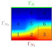
Figure 3. Domain and sample solution ${\bm{u}}({\bm{\mu}})$ for the thermal-block problem.

This section analyzes the performance of the ROMES method on Poisson’s equation with nine system inputs, using the reduced-basis method to generate the reduced-order model. First, Section 5.1 introduces the test problem. Section 5.2 discusses implementation and validation of the ROMES models. Section 5.3 compares the ROMES method to the multifidelity-correction approach characterized by employing the model inputs as error indicators. Section 5.4 compares the ROMES stochastic error estimate to the error bound given by the reduced-basis method. Section 5.5 compares the performance of the two machine-learning algorithms: the Gaussian process kernel method and the relevance vector machine. Finally, Section 5.6 considers non-compliant and multiple output functionals, which ROMES handles via dual-weighted-residual error indicators.

5.1. Problem setup

Consider a finite-element model of heat transport on a square domain $\Omega\vcentcolon=\cup_{i=1}^{9}\Omega_{i}$ composed of nine parameterized materials. The block is cooled along the top boundary to a reference temperature of zero, a nonzero heat flux is specified on the bottom boundary, and the leftmost boundary is adiabatic. The compliant output functional for this problem is defined as the integral over the Neumann domain $\Gamma_{N_{1}}$

(40) $$\bar{g}(u({\bm{\mu}}))=\int_{\Gamma_{N_{1}}}u({\bm{\mu}})\text{d}x,\quad{\bm{\mu}}\in{\mathcal{P}},$$

where the parameter domain is set to ${\mathcal{P}}=[0.1,10]^{9}$ and $u$ is the continuous representation of the finite-element solution. The state variable $u({\bm{\mu}})\in X=H^{1}_{0}\vcentcolon=\left\{w\in H^{1}(\Omega)\;|\;w|_{\Gamma_{D}}=0\right\}$ fulfills the weak form of the parameterized Poisson’s equation: find $u({\bm{\mu}})\in X$, such that

(41) $$a(u({\bm{\mu}}),v)=f(v)\quad\text{for all }v\in X.$$

Here, the bilinear form $a:X\times X\to X$ and the functional $f:X\to X$ are defined as

(42) $$a(u,v)\vcentcolon=\int_{\Omega}b(x;{\bm{\mu}})\nabla u({\bm{\mu}})\cdot\nabla v\,\text{d}x,\qquad f(v)\vcentcolon=\int_{\Gamma_{N_{1}}}v\,\text{d}x$$

with boundary conditions

(43) $$\nabla b(x;{\bm{\mu}})u({\bm{\mu}})\cdot n=0\quad\text{on }\Gamma_{N_{0}},\qquad\nabla b(x;{\bm{\mu}})u({\bm{\mu}})\cdot n=1\quad\text{on }\Gamma_{N_{1}}.$$

We define the coefficient function $b:\Omega\times{\mathcal{P}}\to\mathbb{R}$ as

(44) $$b(x;{{{\bm{\mu}}}})=\sum_{i=1}^{9}\mu_{i}{\mathbbm{1}}_{\Omega_{i}}\left(x\right),$$

where $\mu_{i}$ denotes the $i$th component of the parameter vector ${{{\bm{\mu}}}}$, and the indicator function ${\mathbbm{1}}_{A}\left(x\right)=1$ if $x\in A$ and is zero otherwise. Figure 3 depicts the composition of the domain and the location of the boundary conditions.

By replacing the infinite-dimensional function space $X$ with the (finite) $n$-dimensional finite-element space $X_{\text{h}}\subset X$ in problem (41), one can compute the parameter-dependent state function ${u_{\text{h}}}({\bm{\mu}})\in X_{\text{h}}$ represented by vectors containing the function’s degrees of freedom ${\bm{u}}({{{\bm{\mu}}}})\in\mathbb{R}^{n}$ (see Section A.1). In the experiments, the domain is discretized by triangular finite elements, which results in a finite-element space $X_{\text{h}}$ of dimension $n=10^{4}$. The high-fidelity output (in the notation of Section 2.1) is then $g({\bm{u}}({\bm{\mu}}))\vcentcolon=\bar{g}(u_{\text{h}}({\bm{\mu}}))$, ${\bm{\mu}}\in{\mathcal{P}}$.

As described in Section A.4, we employ a greedy algorithm to generate a reduced-basis space $X_{\text{red}}\subset X_{\text{h}}$ of dimension $p\ll n$. The algorithm employs a training set of $100$ randomly selected points (i.e., $\mathrm{card}\left({\mathcal{P}}_{\mathrm{greedy}}\right)=100$ in Section A.4), until the maximum computed error bound in the training set is less than $1$; it stops after $p=11$ iterations.

Replacing $X_{\text{h}}$ with $X_{\text{red}}$ in Eq. (41) leads to reduced state functions ${u_{\text{red}}}({{{\bm{\mu}}}})\in X_{\text{red}}$ for all ${\bm{\mu}}\in{\mathcal{P}}$. As before, these solutions can be represented by vectors ${\bm{u}}_{\text{red}}({{{\bm{\mu}}}})\vcentcolon=\bm{V}\hat{\bm{u}}({{{\bm{\mu}}}})\in\mathbb{R}^{n}$, where $\bm{V}\in\mathbb{R}^{n\times p}$ is the discrete representation of a basis for the function space $X_{\text{red}}$.

In the following, we analyze two types of error: (i) the energy norm of the state-space error ${\left|\kern-1.07639pt\left|\kern-1.07639pt\left|{\bm{\delta}_{{\bm{u}}}}\right|\kern-1.07639pt\right|\kern-1.07639pt\right|}={\left|\kern-1.07639pt\left|\kern-1.07639pt\left|{\bm{u}}-{\bm{u}}_{\text{red}}\right|\kern-1.07639pt\right|\kern-1.07639pt\right|}\vcentcolon=a({u_{\text{h}}}-{u_{\text{red}}},{u_{\text{h}}}-{u_{\text{red}}})$ and (ii) the output error $\delta_{s}=g({u_{\text{h}}})-g({u_{\text{red}}})$. Because the output functional in this case is compliant (i.e., $g=f$ and $a$ is symmetric), the output error is always non-negative; see Eq. (70) of Section A.3. For more details regarding the finite-element discretization, the reduced-order-model generation, and error bounds, consult Section A of the Supplementary Materials.

5.2. ROMES implementation and validation

We first compute ROMES surrogates for the two errors ${\left|\kern-1.07639pt\left|\kern-1.07639pt\left|{\bm{\delta}_{{\bm{u}}}}\right|\kern-1.07639pt\right|\kern-1.07639pt\right|}$ and (compliant) $\delta_{s}{}$. As proposed in Section 3.2.1, the three ROMES ingredients we employ are: 1) log-residual-norm error indicators $\bm{\rho}({{{\bm{\mu}}}})=\log({r}({\bm{\mu}}))$, 2) a logarithmic transformation function $d=\log$, and 3) both the GP kernel and the RVM supervised machine-learning methods. To train the surrogates, we compute ${\left|\kern-1.07639pt\left|\kern-1.07639pt\left|{\bm{\delta}_{{\bm{u}}}}({\bm{\mu}})\right|\kern-1.07639pt\right|\kern-1.07639pt\right|}$, $\delta_{s}{({\bm{\mu}})}$, and $\bm{\rho}({\bm{\mu}})$ for ${\bm{\mu}}\in\bar{\mathcal{P}}\subset{\mathcal{P}}$ with $\mathrm{card}\left(\bar{\mathcal{P}}\right)=2000$. The first $N=100$ points comprise the ROMES training set $\{{{{\bm{\mu}}}}_{1},\ldots,{{{\bm{\mu}}}}_{N}\}=\vcentcolon{\mathcal{P}}_{\mathrm{learn}}\subset\bar{\mathcal{P}}$ and the following $1900$ points define a validation set ${\mathcal{P}}_{\mathrm{validation}}\subset\bar{\mathcal{P}}$; note that the validation set was not used to construct the error surrogates. Reported results relate to statistics computed over this validation set.

For the kernel method, we employ the squared exponential covariance kernel (30). For the RVM method, we choose Legendre polynomials $P_{k}$ as basis functions, as we expect a linear relationship between the indicators and true errors (see Section 4.2). Because Legendre polynomials are defined on the interval $[-1,1]$, we must transform and scale this domain to span the possible range of indicator values. For this purpose, we apply the heuristic of setting the domain of the polynomials to be 20% larger than the interval bounded by the smallest and largest indicator values:

(45) $$\left[\bm{\rho}_{\min}-0.1(\bm{\rho}_{\max}-\bm{\rho}_{\min}),\bm{\rho}_{\max}+0.1(\bm{\rho}_{\max}-\bm{\rho}_{\min})\right],$$

where $\bm{\rho}_{\min}=\min_{{\bm{\mu}}\in{\mathcal{P}}_{\mathrm{learn}}}\bm{\rho}({\bm{\mu}})$ and $\bm{\rho}_{\max}=\max_{{\bm{\mu}}\in{\mathcal{P}}_{\mathrm{learn}}}\bm{\rho}({\bm{\mu}})$. We include Legendre polynomials of orders $0$ to $4$; however, the RVM method typically discards the higher order polynomials due to the near-linear relation between indicators and errors.

Figure 4. Visualization of ROMES surrogates ($\delta={\left|\kern-1.07639pt\left|\kern-1.07639pt\left|{\bm{\delta}_{{\bm{u}}}}\right|\kern-1.07639pt\right|\kern-1.07639pt\right|}$ and $\left\|{\bm{\delta}_{{\bm{u}}}}\right\|_{X}$, $\bm{\rho}=\log{{r}}$, $d=\log$), computed using $N=100$ training points and the (i) GP kernel method and (ii) RVM.

Figure 4 depicts the ROMES surrogate $\widetilde{{\left|\kern-1.07639pt\left|\kern-1.07639pt\left|{\bm{\delta}_{{\bm{u}}}}\right|\kern-1.07639pt\right|\kern-1.07639pt\right|}}$ generated by both machine-learning methods using all $100$ training points. For comparison, we also create ROMES surrogates $\widetilde{\left\|{\bm{\delta}_{{\bm{u}}}}\right\|_{X}}$ for errors in the parameter-independent norm $\left\|\cdot\right\|_{X}$ of the state space $X=H^{1}_{0}$. In addition to the expected mean of the inferred surrogate, the figure displays two $95\%$-confidence intervals for the prediction (see Remark 4.1):

• The darker shaded interval corresponds to the confidence interval arising from the inherent uncertainty in the error due to the non-uniqueness of the mapping $\bm{\rho}\mapsto{\left|\kern-1.07639pt\left|\kern-1.07639pt\left|{\bm{\delta}_{{\bm{u}}}}\right|\kern-1.07639pt\right|\kern-1.07639pt\right|}$, i.e., the inferred variance $\sigma^{2}$ of Eq. (32).

• The lighter shaded interval also includes the ‘uncertainty in the mean’ due to a lack of training data, i.e., $\Sigma$ of Eq. (32). With an increasing number of training points, this area should be indistinguishable from the darker one.

All ROMES models find a linear trend between the indicators and the errors, where the variance is slightly larger for the parameter-independent norm. This larger variance can be attributed to the larger range of the coercivity constants the parameter-independent norm (see Section A.3). For this example, however, both ROMES are functional. In the following examples, we focus on the energy norm only.

Note that the ‘uncertainty in the mean’ is dominant for the RVM surrogate. This can be explained as follows: the high-order polynomials have values close to zero near the mean of the data. As such, the training data are not very informative for the coefficients of these polynomials. This results in a large inferred variance for those coefficients. Section 5.5 further compares the two machine-learning methods; due to its superior performance, we now proceed with the kernel method.

We now assess the validity of the Gaussian-process assumptions underlying the ROMES surrogates $\widetilde{{\left|\kern-1.07639pt\left|\kern-1.07639pt\left|{\bm{\delta}_{{\bm{u}}}}\right|\kern-1.07639pt\right|\kern-1.07639pt\right|}}$ and $\widetilde{\delta_{s}}$, i.e., Condition 3 of Section 3.1. From the discussion in Remark 4.1, we know if the underlying GP model form is correct, then as the number of training points increases, the uncertainty about the mean decreases and the set $\left\{D({\bm{\mu}})\ |\ {\bm{\mu}}\in{\mathcal{P}}_{\mathrm{validation}}\right\}$ with

(46) $$D({\bm{\mu}})\vcentcolon=d\left({\left|\kern-1.07639pt\left|\kern-1.07639pt\left|{\bm{\delta}_{{\bm{u}}}}({\bm{\mu}})\right|\kern-1.07639pt\right|\kern-1.07639pt\right|}\right)-\mathrm{E}\left[d\left(\widetilde{{\left|\kern-1.07639pt\left|\kern-1.07639pt\left|{\bm{\delta}_{{\bm{u}}}}\right|\kern-1.07639pt\right|\kern-1.07639pt\right|}}(\bm{\rho}({\bm{\mu}}))\right)\right]=d\left({\left|\kern-1.07639pt\left|\kern-1.07639pt\left|{\bm{\delta}_{{\bm{u}}}}({\bm{\mu}})\right|\kern-1.07639pt\right|\kern-1.07639pt\right|}\right)-\nu\left(\bm{\rho}({\bm{\mu}})\right)$$

should behave like samples from the distribution ${\mathcal{N}}(0,\sigma^{2})$. Figure 5 reports this validation test and verifies that this condition does indeed hold for a sufficiently large number of training points.

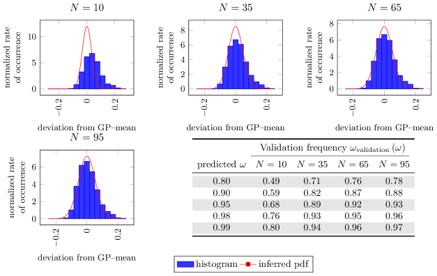
Figure 5. Gaussian-process validation for the ROMES surrogate (GP kernel, $\delta={\left|\kern-1.07639pt\left|\kern-1.07639pt\left|{\bm{\delta}_{{\bm{u}}}}\right|\kern-1.07639pt\right|\kern-1.07639pt\right|}$, $\bm{\rho}=\log{{r}}$, $d=\log$) with a varying number of training points $N$. The histogram corresponds to samples of $D({\bm{\mu}})$ and the red curve depicts the probability distribution function $\mathcal{N}(0,\sigma^{2})$. The table reports how often the actual error lies in the inferred confidence intervals.

Further, we can validate the inferred confidence intervals as proposed in Eq. (9). The table within Figure 5 reports ${{\omega}_{\text{validation}}\left({\omega}\right)}$ (see Eq. (10)), which represents the frequency of observed predictions in the validation set that lie within the inferred confidence interval $C_{{\omega}}$. We declare the ROMES model to be validated, as ${{\omega}_{\text{validation}}\left({\omega}\right)}\approx{\omega}$ for several values of ${\omega}$ as the number of training points increases.

The results for the ROMES surrogate $\widetilde{\delta_{s}{}}$ are very similar to those presented in Figure 5 and will be further discussed in Section 5.3. Note that the inferred Gaussian process is well-converged with a moderately sized training set consisting of only $N=35$ points.

5.3. Output error: comparison with multifidelity correction

As discussed in Section 3.2, multifidelity-correction methods construct a surrogate $\widetilde{\delta_{s,\text{MF}}}$ of the output error using the system inputs as error-surrogate inputs, i.e., $\delta=\delta_{s}$, $\bm{\rho}={{{\bm{\mu}}}}$, and $d=\mathrm{id}_{\mathbb{R}{}}$. In this section, we construct this multifidelity correction surrogate using the same GP kernel method as ROMES. Ref. [35] demonstrated that this error surrogate fails to improve the ‘corrected output’ when the low-fidelity model corresponds to a reduced-order model. We now verify this result and show that—in contrast to the multifidelity correction approach—the ROMES surrogate $\widetilde{\delta_{s}}$ constructed via the GP kernel method with $\delta=\delta_{s}$, $\bm{\rho}=\log{{r}}$, and $d=\log$ yields impressive results: on average, the output ‘corrected’ by the ROMES surrogate reduces the error by an order of magnitude, and the Gaussian-process assumptions can be validated. The validation quality improves as the number of training points increases, but a moderately sized set of only $N=20$ training points leads to a converged surrogate.

Figure 6. Relationship between (i) ROMES error indicators and the compliant-output error and (ii) the first two parameter components and the (compliant) output error, visualized by evaluation of 200 random sample points in the input space. Clearly, the observed structure in the former relationship is more amenable to constructing a Gaussian process.

The reason multifidelity correction fails for most reduced-order models is twofold. First, the mapping ${\bm{\mu}}\mapsto\delta_{s}$ can be highly oscillatory in the input space. This behavior arises from the fact the the reduced-order model error is zero at the (greedily-chosen) ROM training points but grows (and can grow quickly) away from these points. Such complex behavior requires a large number of error-surrogate training points to accurately capture. In addition, the number of system inputs is often large (in this case nine); this introduces curse-of-dimensionality difficulties in modeling the error. Figure 6(ii) visualizes this problem. The depicted mapping between the first two parameter components $\mu_{1},\mu_{2}$ and the output error $\delta_{s}({\bm{\mu}})$ displays no structured behavior. As a result, there is no measurable improvement of the corrected output $s_{\text{red}}{}+\widetilde{\delta_{s,\text{MF}}{}}$ over the evaluation of the ROM output $s_{\text{red}}$ alone.

In order to quantify the performance of the error surrogates, we introduce a normalized expected improvement

(47) $$I(\widetilde{\delta},{\bm{\mu}})\vcentcolon=\left|\frac{\delta_{s}{({\bm{\mu}})}-\mathrm{mode}\left(\widetilde{\delta{}}(\bm{\rho}({\bm{\mu}}))\right)}{\delta_{s}{({\bm{\mu}})}}\right|.$$

If this value is less than one, then the exected corrected output $s_{\text{red}}{}+\widetilde{\delta{}}$ is more accurate than the ROM output $s_{\text{red}}{}$ itself for point ${\bm{\mu}}\in{\mathcal{P}}$, i.e., the additive error surrogate improves the prediction of the ROM. On the other hand, values above one indicate that the error surrogate worsens the ROM prediction.

Figure 7 reports the mean, median, standard deviations, and extrema for the expected improvement (47) evaluated for all validation points ${\mathcal{P}}_{\mathrm{validation}}$ and a varying number of training points. Here, we also compare with the performance of the error surrogate $\widetilde{\delta_{\text{uni}}}$, which is defined as a uniform distribution on the interval $\left[\Delta^{\text{LB}}_{s}{({\bm{\mu}})},\Delta_{s}{({\bm{\mu}})}\right]$, where $\Delta^{\text{LB}}_{s}{({\bm{\mu}})}$ and $\Delta_{s}{({\bm{\mu}})}$ are the the lower and upper bounds for the output error, respectively. Note that $\widetilde{\delta_{\text{uni}}}$ does not require training data, as it is based purely on error bounds.

The expected improvement for the ROMES output-error surrogate $I(\widetilde{\delta_{s}{}},{\bm{\mu}})$ as depicted in Figure 7(i) is approximately $0.2$ on average, which constitutes an improvement of nearly an order of magnitude. Further, the maximum expected improvement almost always remains below $1$; this implies that the corrected ROM output is almost always more accurate than the ROM output alone.

On the other hand, the expected improvement generated by the error surrogate $\widetilde{\delta_{\text{uni}}}$ is always greater than one, which means that its correction always increases the error. This arises from the fact that the center of the interval $\left[\Delta^{\text{LB}}_{s}{({\bm{\mu}})},\Delta_{s}{({\bm{\mu}})}\right]$ is a poor approximation for the true error.

In addition, Figure 7(ii) shows that the expected improvement produced by the multifidelity-correction surrogate $I\left(\widetilde{\delta_{s,\text{MF}}},{\bm{\mu}}\right)$ is often far greater than one. This shows that the multifidelity-correction approach is not well suited for this problem. Presumably, with (far) more training points, these results would improve.

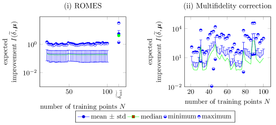
Figure 7. Expected improvement $I(\widetilde{\delta},{\bm{\mu}})$ for a varying number of training points $N$: (i) ROMES (GP kernel, compliant $\delta=\delta_{s}$, $\bm{\rho}=\log{{r}}$, $d=\log$) with uniform distribution based on reduced-basis error bounds $\widetilde{\delta_{\text{uni}}}$ and (ii) multifidelity correction (GP kernel, compliant $\delta=\delta_{s}$, $\bm{\rho}={{{\bm{\mu}}}}$, and $d=\mathrm{id}_{\mathbb{R}{}}$). ($1$: no improvement, $>1$: error worsened, ${}<1$: error improved).

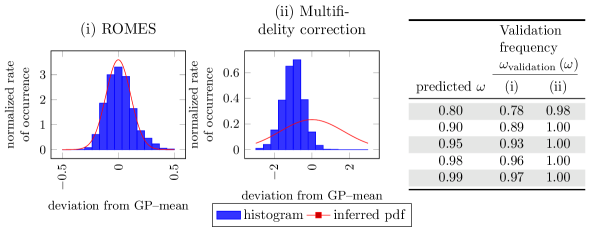
Figure 8. Gaussian-process validation for the ROMES surrogate (GP kernel, compliant $\delta=\delta_{s}$, $\bm{\rho}=\log{{r}}$, $d=\log$) and multifidelity-correction surrogate (GP kernel, compliant $\delta=\delta_{s}$, $\bm{\rho}={{{\bm{\mu}}}}$, and $d=\mathrm{id}_{\mathbb{R}{}}$) using $N=100$ training points The histogram corresponds to samples of $D({\bm{\mu}})$ and the red curve depicts the probability distribution function $\mathcal{N}(0,\sigma^{2})$. The table reports how often the actual error lies in the inferred confidence intervals. Clearly, this validation test fails for the multilfidelity-correction surrogate.

Again, we can validate the Gaussian-process assumptions underlying the error surrogates. For $N=100$ training points, Figure 8 compares a histogram of deviation of the true error from the surrogate mean to the inferred probability density function. The associated table reports how often the validation data lie in inferred confidence intervals. We observe that the confidence intervals are valid for the ROMES surrogate, but are not for the multifidelity-correction surrogate, as the bins do not align with the inferred distribution. Figure 9 depicts the convergence of these confidence-interval validation metrics as the number of training points increases. As expected (see Remark 4.1) the ROMES observed confidence intervals more closely align with the confidence intervals arising from the inherent uncertainty (i.e., $\sigma^{2}$) as the number of training points increases, as this effectively decreases the uncertainty due to a lack of training. In addition, only a moderate number of training points (around $20$) is required to generate a reasonably converged ROMES surrogate. On the other hand the multifidelity-correction surrogate exhibits no such convergence when fewer than 100 training points are used.

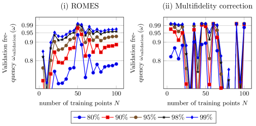
Figure 9. Gaussian-process validation for the ROMES surrogate (GP kernel, compliant $\delta=\delta_{s}$, $\bm{\rho}=\log{{r}}$, $d=\log$) and multifidelity-correction surrogate (GP kernel, compliant $\delta=\delta_{s}$, $\bm{\rho}={{{\bm{\mu}}}}$, and $d=\mathrm{id}_{\mathbb{R}{}}$) and a varying number of training points $N$. The plots depict how often the actual error lies in the inferred confidence intervals.

5.4. Reduced-basis error bounds

In this section, we compare the reduced-basis error bound $\Delta_{{\bm{u}}}^{{\bm{\mu}}}$ (64) with the probabilistically rigorous ROMES surrogates $\widetilde{{\left|\kern-1.07639pt\left|\kern-1.07639pt\left|{\bm{\delta}_{{\bm{u}}}}\right|\kern-1.07639pt\right|\kern-1.07639pt\right|}}^{c}$ (8) with rigor values of $c=0.5$ and $c=0.9$ as introduced Section 3.3. The ROMES surrogate is constructed with the GP kernel method and ingredients $\delta={\left|\kern-1.07639pt\left|\kern-1.07639pt\left|{\bm{\delta}_{{\bm{u}}}}\right|\kern-1.07639pt\right|\kern-1.07639pt\right|}$, $\bm{\rho}=\log{{r}}$, and $d=\log$. As discussed in Section 2.3 the error-bound effectivity (8) is important to quantify the performance of these bounds; a value of 1 is optimal, as it implies no over-estimation.

As the probabilistically rigorous ROMES surrogates $\widetilde{{\left|\kern-1.07639pt\left|\kern-1.07639pt\left|{\bm{\delta}_{{\bm{u}}}}\right|\kern-1.07639pt\right|\kern-1.07639pt\right|}}^{c}$ are stochastic processes, we can measure their (most common) effectivity as

(48) $$\eta(c,{\bm{\mu}})\vcentcolon={\frac{\mathrm{mode}\left(\widetilde{{\left|\kern-1.07639pt\left|\kern-1.07639pt\left|{\bm{\delta}_{{\bm{u}}}}\right|\kern-1.07639pt\right|\kern-1.07639pt\right|}}^{c}\left(\bm{\rho}({\bm{\mu}})\right)\right)}{{\left|\kern-1.07639pt\left|\kern-1.07639pt\left|{\bm{\delta}_{{\bm{u}}}}({\bm{\mu}})\right|\kern-1.07639pt\right|\kern-1.07639pt\right|}}}.$$

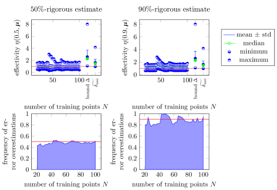
Figure 10. Validation of the probabilistically rigorous ROMES surrogates $\widetilde{{\left|\kern-1.07639pt\left|\kern-1.07639pt\left|{\bm{\delta}_{{\bm{u}}}}\right|\kern-1.07639pt\right|\kern-1.07639pt\right|}}^{c}$ (GP kernel, $\delta={\left|\kern-1.07639pt\left|\kern-1.07639pt\left|{\bm{\delta}_{{\bm{u}}}}\right|\kern-1.07639pt\right|\kern-1.07639pt\right|}$, $\bm{\rho}=\log{{r}}$, $d=\log$) and comparison with RB error upper bound $\Delta_{{\bm{u}}}^{{\bm{\mu}}}$ and uniform distribution based on reduced-basis error bounds $\widetilde{\delta_{\text{uni}}}$. The top plots compare statistics of the effectivities $\eta(c,{\bm{\mu}})$ with $c=0.5$ and $c=0.9$ of the probabilistically rigorous ROMES surrogates with the RB error-bound surrogates. The bottom plots compare the frequency of error overestimation $c_{\text{validation}}$ with the desired value $c$ (red line).

The top plots of Figure 10 report the mean, median, standard deviation, and extrema of the effectivities $\eta(0.5,{\bm{\mu}})$ and $\eta(0.9,{\bm{\mu}})$ for all validation points ${\bm{\mu}}\in{\mathcal{P}}_{\mathrm{validation}}$. Again, we compare with $\widetilde{\delta_{\text{uni}}}$, which is a uniform distribution on an interval whose endpoints correspond to the lower and upper bounds for the error ${\left|\kern-1.07639pt\left|\kern-1.07639pt\left|{\bm{\delta}_{{\bm{u}}}}({\bm{\mu}})\right|\kern-1.07639pt\right|\kern-1.07639pt\right|}$. We also compare with the corresponding statistics for the effectivity of the RB error bound $\Delta_{{\bm{u}}}^{{\bm{\mu}}}$. The lower bound for the coercivity constant that is needed in the RB error bound $\Delta_{{\bm{u}}}^{{\bm{\mu}}}$ is chosen as the minimum over all parameter components $\alpha_{\text{LB}}({\bm{\mu}})=\min_{i\in\{1,\ldots,9\}}\mu_{i}.$ This simple choice is effective because the example is affinely parameter dependent and linear [37, Ch. 4.2].

We observe that the ROMES surrogate yields better results than both the error bound $\Delta_{{\bm{u}}}^{{\bm{\mu}}}$ (which produces effectivities roughly between one and eight) and the uniform distribution $\widetilde{\delta_{\text{uni}}}$ (which produces mode effectivities roughly between one and four). The $50\%$-rigorous ROMES surrogate has an almost perfect mean effectivity of $1$ as desired. The $90\%$-rigorous surrogate has a higher mean effectivity as expected; however, it is only slightly higher. Furthermore, the effectivities of the ROMES surrogate exhibit a much smaller variance than both $\Delta_{{\bm{u}}}^{{\bm{\mu}}}$ and $\widetilde{\delta_{\text{uni}}}$. Finally, a moderate number (around 20) of training samples is sufficient to obtain well-converged surrogates.

The bottom plots of Figure 10 report the frequency of error overestimation

(49) $$c_{\text{validation}}\vcentcolon=\frac{\mathrm{card}\left(\{{\bm{\mu}}\in{\mathcal{P}}_{\mathrm{validation}}\ |\ \mathrm{median}\left(\tilde{m}\left(\bm{\rho}({\bm{\mu}})\right)\right)>d(\delta{({\bm{\mu}})})\}\right)}{\mathrm{card}\left({\mathcal{P}}_{\mathrm{validation}}\right)}$$

for the probabilistically rigorous ROMES surrogates (i.e., $\tilde{m}=\widetilde{{\left|\kern-1.07639pt\left|\kern-1.07639pt\left|{\bm{\delta}_{{\bm{u}}}}\right|\kern-1.07639pt\right|\kern-1.07639pt\right|}}^{c}$) as the number of training points increases to show that $c_{\text{validation}}\approx c$, which validates the rate of error overestimation (see Eq. (23)). Note that the overestimation frequency $c_{\text{validation}}$ converges to its predicted value $c$, which demonstrates that the rigor of the ROMES estimates can in fact be controlled.

5.5. Comparison of machine-learning algorithms

This section compares in detail the ROMES surrogates generated using the two machine-learning methods introduced in Section 4. Recall that Figure 4 visualizes both surrogates. We observe that both methods work well overall and generate well-converged surrogates with a modest number of training samples. As previously mentioned, the GP kernel leads to a smaller inferred variance due to more accurate and localized estimates of the mean. The RVM is characterized by global basis functions that preclude it from accurately resolving localized features of the mean and lead to large uncertainty about the mean (see Figure 4). On the other hand, the confidence intervals computed with the RVM are (slightly) better validated.

Figure 11. Gaussian-process validation for the ROMES surrogate using both the GP kernel method and the RVM ($\delta={\left|\kern-1.07639pt\left|\kern-1.07639pt\left|{\bm{\delta}_{{\bm{u}}}}\right|\kern-1.07639pt\right|\kern-1.07639pt\right|}$, $\bm{\rho}=\log{{r}}$, $d=\log$) using $N=80$ training points. The histogram corresponds to samples of $D({\bm{\mu}})$ and the red curve depicts the probability distribution function $\mathcal{N}(0,\sigma^{2})$. The table reports how often the actual error lies in the inferred confidence intervals.

Figure 11(i) and (ii) report the validation test, i.e., the frequency of deviations from the inferred mean $D({\bm{\mu}})$ (46) with a training sample containing $N=80$ training points. We observe a smaller inferred variance $\sigma^{2}$ for the GP kernel method, which implies that the mean is identified more accurately. In both cases, the validation samples align well with the probability density function of the inferred distribution ${\mathcal{N}}(0,\sigma^{2})$.

The confidence intervals of this inferred distribution can be validated, and they turn out to be (slightly) more realistic for the RVM method. The table within Figure 11 shows that the kernel method results are usually optimistic, i.e., the actual confidence intervals are smaller than predicted. This effect can be corrected, however, by adding $\Sigma(\bm{x}^{*})$ as an indicator of the uncertainty of the mean as discussed in Remark 4.1. However, doing so for the RVM prediction yields extremely wide confidence intervals due to the significant uncertainty about the RVM mean (see Figure 4).

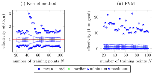
Figure 12. Comparison of the effectivity $\eta(0.5,{\bm{\mu}})$ of ROMES surrogates ($\delta={\left|\kern-1.07639pt\left|\kern-1.07639pt\left|{\bm{\delta}_{{\bm{u}}}}\right|\kern-1.07639pt\right|\kern-1.07639pt\right|}$, $\bm{\rho}=\log{{r}}$, $d=\log$) with the GP computed via (i) the GP kernel and (ii) the relevance vector machine method.

As the inferred variance is larger for the relevance vector machine, this also affects the performance of effectivity and improvement measures for the error surrogates. Figure 12 depicts statistics of $\eta(0.5,{\bm{\mu}})$ computed with both the methods, and we observe that all statistical measures are significantly better for the kernel method estimate.

We conclude that while both methods produce feasible ROMES surrogates, the GP kernel method produces consistently better results. In particular, the lower inferred variance implies that a lower amount of epistemic uncertainty is introduced by the error surrogate (See condition 2 from Section 3.1). This is critically important for many UQ tasks. Therefore, we recommend the GP kernel method to construct ROMES surrogates.

5.5.1. Dependence on reduced-basis size

To assess the generalizability of the ROMES method, we apply it to a ROM of higher fidelity, i.e., larger $p$. We construct two ROMES surrogates: one for the state-space error $\widetilde{{\left|\kern-1.07639pt\left|\kern-1.07639pt\left|{\bm{\delta}_{{\bm{u}}}}\right|\kern-1.07639pt\right|\kern-1.07639pt\right|}}$ (GP kernel, $\delta={\left|\kern-1.07639pt\left|\kern-1.07639pt\left|{\bm{\delta}_{{\bm{u}}}}\right|\kern-1.07639pt\right|\kern-1.07639pt\right|}$, $\bm{\rho}=\log{{r}}$, $d=\log$) and one for the compliant-output error $\widetilde{\delta_{s}}$ (GP kernel, $\delta=\delta_{s}$, $\bm{\rho}=\log{{r}}$, $d=\log$).

We increase the reduced-basis size by decreasing the maximum error over the training set from $1.0$ to $1.0\times 10^{-3}$ and applying the greedy method. The resulting reduced-basis dimension is $p=62$. Figure 13 reports the error data and ROMES surrogates. Comparing the leftmost plot of Figure 13 with Figure 4(i) and the rightmost plot of Figure 13 with Figure 6(i) reveals that while the errors are several orders of magnitude smaller for the current experiments, the data (and the resulting ROMES surrogates) exhibit roughly the same structure as before.

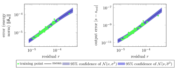
Figure 13. Visualization of ROMES surrogates ($\delta={\left|\kern-1.07639pt\left|\kern-1.07639pt\left|{\bm{\delta}_{{\bm{u}}}}\right|\kern-1.07639pt\right|\kern-1.07639pt\right|}$ and $\delta_{s}{}$, $\bm{\rho}=\log{{r}}$, $d=\log$), computed using $N=100$ training points and the GP kernel method for a higher dimensional ROM with $p=62$.

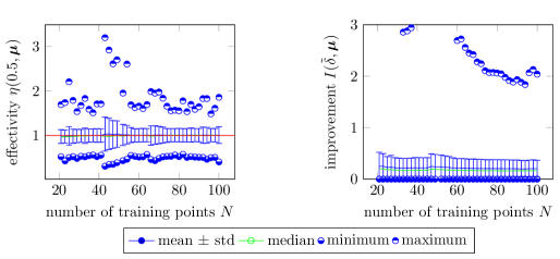
Figure 14. Effectivity $\eta(0.5,{\bm{\mu}})$ of ROMES surrogate ($\delta={\left|\kern-1.07639pt\left|\kern-1.07639pt\left|{\bm{\delta}_{{\bm{u}}}}\right|\kern-1.07639pt\right|\kern-1.07639pt\right|}$, $\bm{\rho}=\log{{r}}$, $d=\log$) and expected improvement $I(\widetilde{\delta},{\bm{\mu}})$ of ROMES surrogate (GP kernel, compliant $\delta=\delta_{s}$, $\bm{\rho}=\log{{r}}$, $d=\log$) for a higher dimensional ROM with $p=62$ and a varying number of training points $N$.

Figure 14 reports the performance of these surrogates. Comparing the leftmost plot of Figure 14 with Figure 12(i) shows that the state-space error surrogate exhibits nearly identical convergence for the larger- and smaller-dimension reduced-order models. As in the experiments of Section 5.4, the value of $\mathrm{mode}\left(\eta(0.5,{\bm{\mu}})\right)$ is close to $1$ in the mean. Comparing the rightmost plot of Figure 14 with Figure 7(i) shows that the expected improvement for the output-error correction with the surrogate $\widetilde{\delta_{s}}$ is around $0.2$ in the mean for both the larger- and smaller-dimension reduced-order models. However, for the larger-dimension reduced-order model, more training points are required to reduce the occurrence of improvement factors larger than $1$. This is an artifact of the low errors already produced by the larger-dimension ROM itself (i.e., small denominator in Eq. (47)).

We therefore conclude that the ROMES method is applicable to ROMs of different fidelity.

5.6. Multiple and non-compliant outputs

Finally, we assess the performance of ROMES on a model with multiple and non-compliant output functionals as discussed in Section 3.2.2. For this experiment, we set two outputs to be temperate measurements at points $x_{1}$ and $x_{2}$:

(50) $$s_{i}\left({\bm{\mu}}\right)\vcentcolon=g_{i}\left({\bm{u}}\left({\bm{\mu}}\right)\right)\vcentcolon=\bar{g}_{i}\left(u\left({\bm{\mu}}\right)\right)=\int_{\Omega}\delta_{\text{Dirac}}(x-x_{i})u\left(x_{i};{\bm{\mu}}\right)\text{d}x=u\left(x_{i};{\bm{\mu}}\right),\quad i=1,2.$$

where $\delta_{\text{Dirac}}$ denotes the Dirac delta function. In this case, we construct a separate ROMES surrogates for each output error $\widetilde{{\delta_{s_{1}}}}$ and $\widetilde{\delta_{s_{2}}}$. As previously discussed, we use dual-weighted residuals as indicators $\bm{\rho}_{i}({\bm{\mu}})=\bm{y}_{\text{red},i}({\bm{\mu}})^{t}\bm{r}\left({\bm{u}}_{\text{red}};{\bm{\mu}}\right)$, $i=1,2$ and no transformation $d\equiv\text{id}_{\mathbb{R}}$. This necessitates the computation of approximate dual solutions, for which dual reduced-basis spaces must be generated in the offline stage. The corresponding finite element problem can be found in Eq. (79), where Eq. (50) above provides the right-hand sides. The algebraic problems can be inferred from Eq. (80), where the discrete right-hand sides are canonical unit vectors because the points $x_{1}$ and $x_{2}$ coincide with nodes of the finite-element mesh.

Like the primal reduced basis, the dual counterpart can be generated with a greedy algorithm that minimizes the approximation error for the reduced dual solutions.

To assess the ability for uncertainty control with the dual-weighted-residual indicators (see Remark 3.2) we generate three dual reduced bases of increasing fidelity: 1) error tolerance of $1$ (basis sizes $p_{y}$ of 10 and 11), 2) error tolerance of $0.5$ (basis sizes $p_{y}$ of 15 and 17), 3) error tolerance of $0.1$ (basis sizes $p_{y}$ of 20 and 23).

To train the surrogates, we compute $\delta_{s_{1}}{({\bm{\mu}})}$, $\delta_{s_{2}}{({\bm{\mu}})}$, $\bm{\rho}_{1}({\bm{\mu}})$ (of varying fidelity), $\bm{\rho}_{2}({\bm{\mu}})$ (of varying fidelity), for ${\bm{\mu}}\in\bar{\mathcal{P}}\subset{\mathcal{P}}$ with $\mathrm{card}\left(\bar{\mathcal{P}}\right)=500$. The first $T=100$ points define the training set ${\mathcal{P}}_{\mathrm{learn}}\subset\bar{\mathcal{P}}$ and the following $400$ points constitute the validation set ${\mathcal{P}}_{\mathrm{validation}}\subset\bar{\mathcal{P}}$.

Figure 15 depicts the observed relationship between indicators $\bm{\rho}_{1}({\bm{\mu}})$ (of different fidelity) and the error in the first output $\delta_{s_{1}}({\bm{\mu}})$. Note that as the dual-basis size $p_{y}$ increases, the output error exhibits a nearly exact linear dependence on the dual-weighted residuals. This is expected, as the residual operator is linear in the state. Therefore, the RVM with a linear polynomial basis produces the best (i.e., minimum variance) results for the ROMES surrogates in this case.

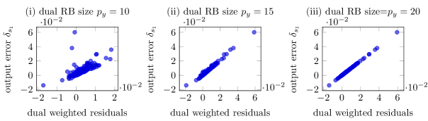
Figure 15. Relationship between between dual-weighted-residual indicators $\bm{\rho}_{1}=\bm{y}_{\text{red},1}({\bm{\mu}})^{t}\bm{r}\left({\bm{u}}_{\text{red}};{\bm{\mu}}\right)$ and errors in the (non-compliant) first output $\delta_{s_{1}}$.

Figure 16 reflects the necessity of employing a large enough dual reduced basis to compute the dual-weighted-residual error indicators. For a small dual reduced basis, there is almost no improvement in the mean, and only a slight improvement in the median; in some cases, the ‘corrected’ outputs are actually less accurate. However, the most accurate dual solutions yield a mean and median error improvement of two orders of magnitude. This illustrates the ability and utility of uncertainty control when dual-weighted residuals are used as error indicators.

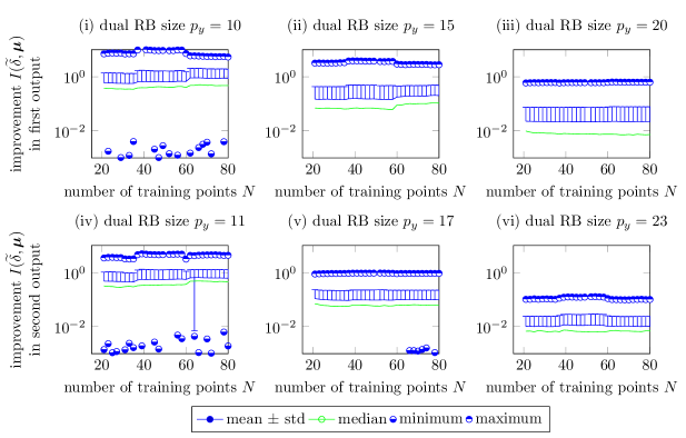
Figure 16. Expected improvement $I(\widetilde{\delta},{\bm{\mu}})$ for ROMES surrogate (RVM, $\delta=\delta_{s}$, $\bm{\rho}_{i}=\bm{y}_{\text{red},i}({\bm{\mu}})^{t}\bm{r}\left({\bm{u}}_{\text{red}};{\bm{\mu}}\right)$, $i=1,2$, $d=\text{id}_{\mathbb{R}}$) for a varying number of training points $T$ and different dual reduced-basis-space dimensions. Compare with Figure 7 (1: no improvement, $>1$: error worsened, $<1$: error improved).

Table 17 reports validation results for the inferred confidence intervals. While the validation results are quite good (and appear to be converging to the correct values), they are not as accurate as those obtained for the compliant output.

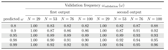
Figure 17. Gaussian-process validation for the ROMES surrogates (RVM, $\delta=\delta_{s}$, $\bm{\rho}_{i}=\bm{y}_{\text{red},i}({\bm{\mu}})^{t}\bm{r}\left({\bm{u}}_{\text{red}};{\bm{\mu}}\right)$, $i=1,2$, $d=\text{id}_{\mathbb{R}}$). The table reports how often the actual error lies in the inferred confidence intervals. The largest dual reduced-basis space dimensions ($p_{y}=20$ and $p_{y}=23$) are used to compute the error indicators. .

6. Conclusions and outlook

This work presented the ROMES method for statistically modeling reduced-order-model errors. In contrast to rigorous error bounds, such statistical models are useful for tasks in uncertainty quantification. The method employs supervised machine learning methods to construct a mapping from existing, cheaply computable ROM error indicators to a distribution over the true error. This distribution reflects the epistemic uncertainty introduced by the ROM. We proposed ROMES ingredients (supervised-learning method, error indicators, and transformation function) that yield low-variance, numerically validated models for different types of ROM errors.

For normed outputs, the ROMES surrogates led to effectivities with low variance and means close to the optimal value of one, as well as a notion of probabilistic rigor. This is in contrast to existing ROM error bounds, which exhibited mean effectivities close to ten; this improvement will likely be more pronounced for more complex (e.g., nonlinear, time dependent) problems. Further, the ROMES surrogates were computationally less expensive than the error bounds, as the coercivity-constant lower bound was not required.

For general outputs, the ROMES surrogate allowed the ROM output to be corrected, which yielded a near 10x accuracy improvement. Further, the uncertainty in this error could be controlled by modifying the dimension of the dual reduced basis. On the other hand, existing approaches (i.e., multifidelity correction) that employ system inputs (not error indicators) as inputs to the error model did not lead to improved output predictions. This demonstrated the ability of ROMES to mitigate the curse of dimensionality: although the problem was characterized by nine system inputs, only one error indicator was necessary to construct a low-variance, validated ROMES surrogate.

We foresee the combination of ROMs with ROMES error surrogates to be powerful in UQ applications, especially when the number of system inputs is large. Future work entails integrating and analyzing the ROM/ROMES combination for specific UQ problems, e.g., Bayesian inference, as well as automating the procedure for selecting ROMES ingredients for different problems. Future work will also involve integrating the ROMES surrogates into the greedy algorithm for the reduced-basis-space selection; this has the potential to improve ROM quality due to the near-optimal expected effectivities of the error surrogates.

Appendix A Reduced-basis method for parametric elliptic PDEs with affine parameter dependence

This section summarizes the reduced-basis method for generating a reduced-order model for parametric elliptic PDEs with affine parameter dependence. See Ref. [37] for additional details.

A.1. Parametric elliptic problem

We start with the discretized version of the elliptic problem, where the state resides in a function space $X_{\text{h}}\subset X$ of finite dimension $n\vcentcolon=\dim(X_{\text{h}})$, e.g., a finite-element space. For details on the derivation of such a finite element discretization from the analytical formulation of an elliptic PDE and its convergence properties, we refer to Ref. [9].

The problem reads as follows: For any point in the input space ${\bm{\mu}}\in{\mathcal{P}}$, compute a quantity of interest

(51) $$s({\bm{\mu}}) \vcentcolon=\bar{g}(u_{\text{h}}({\bm{\mu}}))$$

with $$u_{\text{h}}\in X_{\text{h}}$$ fulfilling

(52) $$a(u_{\text{h}}({\bm{\mu}}),v_{\text{h}};{\bm{\mu}}) =f(v_{\text{h}};{\bm{\mu}})\ \text{for all }v_{\text{h}}\in X_{\text{h}}.$$

Here, for all inputs ${\bm{\mu}}\in{\mathcal{P}}$, $a(\cdot,\cdot;{\bm{\mu}}):X_{\text{h}}\times X_{\text{h}}\to X_{\text{h}}$ is a bilinear form on a Hilbert space $X_{\text{h}}$ and is symmetric, continuous, and coercive, fulfilling

(53) $$\sup_{u\in X}\sup_{v\in X}\frac{a(u,v;{\bm{\mu}})}{\left\|u\right\|_{X}\left\|v\right\|_{X}}<\gamma({\bm{\mu}})<\infty\quad\text{ and }\inf_{u\in X,\left\|u\right\|_{X}=1}a(u,u;{\bm{\mu}})>\alpha({\bm{\mu}})$$

for constants $\gamma({\bm{\mu}})$ and $\alpha({\bm{\mu}})>0$. In addition, we have $f({\bm{\mu}})\in X^{*}_{\text{h}}$.

Given a basis $\left\{\varphi_{i}\right\}_{i=1}^{n}$ spanning $X_{\text{h}}$, the solution can be expressed as a linear combination $u_{\text{h}}({\bm{\mu}})=\sum_{i=1}^{n}{u}_{i}({\bm{\mu}})\varphi_{i}\in X_{\text{h}}$ with the state vector ${\bm{u}}\vcentcolon=\left[u_{1}\ \cdots\ u_{n}\right]^{t}:{\mathcal{P}}\rightarrow\mathbb{R}^{n}$ containing the solution degrees of freedom. Then, problem (52) can be solved algebraically by solving the system of linear equations

(54) $$\bm{r}({\bm{u}};{\bm{\mu}})\vcentcolon=\mathbf{A}({\bm{\mu}}){\bm{u}}({\bm{\mu}})-\mathbf{f}({\bm{\mu}})=0,$$

with $\mathbf{A}:{\mathcal{P}}\rightarrow\mathbb{R}^{n\times n}$ given by $\mathbf{A}_{ij}({\bm{\mu}})=a\left(\varphi_{i},\varphi_{j};{\bm{\mu}}\right)$ and $\mathbf{f}:{\mathcal{P}}\rightarrow\mathbb{R}^{n}$ given by $\mathbf{f}_{i}({\bm{\mu}})=f(\varphi_{i};{\bm{\mu}})$. Similarly, the output can be expressed as a function of the state degrees of freedom:

(55) $$g({\bm{u}}({\bm{\mu}}))\vcentcolon=\bar{g}\left(\sum_{i=1}^{n}{u}_{i}({\bm{\mu}})\varphi_{i}\right).$$

The key concept underlying projection-based model-reduction techniques is to find a lower dimensional subspace $X_{\text{red}}\subset X_{\text{h}}$ of dimension $p:=\dim(X_{\text{red}})\ll n$, such that (54) can be solved more efficiently. For the reduced-basis method, this problem-dependent reduced-basis space is obtained through identification of a few training points ${\mathcal{P}}_{\mathrm{train}}\vcentcolon=\left\{\tilde{\bm{\mu}}_{i}\right\}_{i=1}^{p}\subset{\mathcal{P}}$ for which the full-order equations (54) are solved. These functions then span the reduced basis space $X_{\text{red}}=\mathrm{span}\left\{u(\tilde{\bm{\mu}}_{i})\right\}_{i=1}^{p}$ from which we generate an orthonormal basis $\left\{\psi_{i}\right\}_{i=1}^{p}.$ We refer to subsection A.4 for more details on the selection process of these parameters. Then, these basis vectors can be expressed in terms of the original finite-element degrees of freedom, i.e.,

(56) $$\psi_{j}=\sum_{i=1}^{n}\varphi_{i}\bm{V}_{ij},\quad j=1,\ldots,p.$$

This transformation provides the entries of the trial basis $\bm{V}$. As we consider only Galerkin projection (due to the symmetric and coercive nature of the PDE), we set $\bm{W}=\bm{V}$, which leads to a reduced-order problem of the form (4):

(57) $$\bm{V}^{t}\bm{r}(\bm{V}\hat{\bm{u}};{\bm{\mu}})=\bm{V}^{t}\mathbf{A}({\bm{\mu}})\bm{V}\hat{\bm{u}}({\bm{\mu}})-\bm{V}^{t}\mathbf{f}({\bm{\mu}})\bm{V}=0.$$

The reduced quantity of interest is then given by $s_{\text{red}}{}=g(\bm{V}\hat{\bm{u}}).$

A.2. Offline–online decomposition

The low-dimensional operators in Eq. (57) can be computed efficiently assuming that the bilinear forms $a$ and the functional $f$ are affinely parameter dependent, i.e., they can be written as

(58) $$a(\cdot,\cdot;{\bm{\mu}})=\sum_{q=1}^{Q_{a}}\sigma_{a}^{q}({\bm{\mu}})a^{q}(\cdot,\cdot)\quad\text{and}\quad f(\cdot;{\bm{\mu}})=\sum_{q=1}^{Q_{f}}\sigma_{f}^{q}({\bm{\mu}})f^{q}(\cdot).$$

with parameter-independent bilinear forms $a^{q}:X_{h}\times X_{h}\to X_{h},q=1,\ldots,Q_{a}$ and functionals $f^{q}:X_{h}\to X_{h},q=1,\ldots,Q_{f}$, and coefficient functions $\sigma_{a}^{q}:{\mathcal{P}}\to\mathbb{R},q=1,\ldots,Q_{a}$ and $\sigma_{f}^{q}:{\mathcal{P}}\to\mathbb{R},q=1,\ldots,Q_{f}$.

In this affinely parameter dependent case, the parameter-dependent reduced quantities $\bm{V}^{t}\mathbf{A}({\bm{\mu}})\bm{V}$ and $\bm{V}^{t}\mathbf{f}({\bm{\mu}})\bm{V}$ can be quickly assembled via a linear combination of their parameter-independent components:

(59) $$\bm{V}^{t}\mathbf{A}({\bm{\mu}})\bm{V}=\sum_{q=1}^{Q_{a}}\sigma^{q}_{a}({\bm{\mu}})\bm{V}^{t}\mathbf{A}^{q}\bm{V}$$

(60) $$\bm{V}^{t}\mathbf{f}\bm{V}=\sum_{q=1}^{Q_{f}}\sigma^{q}_{f}({\bm{\mu}})\bm{V}^{t}\mathbf{f}^{q}\bm{V}.$$

Here the matrices $\mathbf{A}^{q}\in\mathbb{R}^{n\times n},q=1,\ldots,Q_{a}$ are given by $\mathbf{A}^{q}_{ij}=a^{q}(\varphi_{i},\varphi_{j})$ and the vectors $\mathbf{f}^{q}\in\mathbb{R}^{n},q=1,\ldots,Q_{f}$ are given by $\mathbf{f}^{q}_{i}=f(\varphi_{i})$.

The parameter-independent components

(61) $$\bm{V}^{t}\mathbf{A}^{q}\bm{V}\in\mathbb{R}^{p\times p},\ q=1,\ldots,Q_{a}\qquad\text{and}\qquad\bm{V}^{t}\mathbf{f}^{q}\bm{V}\in\mathbb{R}^{p},\ q=1,\ldots,Q_{f}$$

must be computed only once, during the so-called offline stage. All parameter-dependent computations are carried out in the online stage in an efficient manner, i.e., with computational complexities that only depend on the reduced-basis dimension $p$. We refer to Ref. [37] for more details on the offline/online decomposition. Note that in the non-affine case, low-dimensional operators can be approximated using the empirical interpolation method [6, 28, 16].

A.3. Error bounds

The state error can be measured either in the problem–dependent energy norm or in the norm given by the underlying Hilbert space $X_{\text{h}}$. The energy norm for the above problem is defined as

(62) $${\left|\kern-1.07639pt\left|\kern-1.07639pt\left|u\right|\kern-1.07639pt\right|\kern-1.07639pt\right|}\vcentcolon=a(u,u;{{{\bm{\mu}}}})$$

and is equivalent to the $X_{h}$-norm

(63) $$\alpha\left\|u\right\|_{X_{\text{h}}}^{2}\leq{\left|\kern-1.07639pt\left|\kern-1.07639pt\left|u\right|\kern-1.07639pt\right|\kern-1.07639pt\right|}^{2}\leq\gamma\left\|u\right\|_{X_{\text{h}}}^{2}.$$

The bounds for the state errors $\Delta_{{\bm{u}}}^{{\bm{\mu}}}$ and $\Delta_{{\bm{u}}}$ for the errors ${\left|\kern-1.07639pt\left|\kern-1.07639pt\left|{\bm{\delta}_{{\bm{u}}}}\right|\kern-1.07639pt\right|\kern-1.07639pt\right|}$ and $\left\|{\bm{\delta}_{{\bm{u}}}}\right\|_{X_{\text{h}}}$ are defined as follows:

(64) $$\Delta_{{\bm{u}}}^{{\bm{\mu}}}({\bm{\mu}}) \vcentcolon=\frac{r({\bm{\mu}})}{\sqrt{\alpha_{\text{LB}}({\bm{\mu}})}} \geq{\left|\kern-1.07639pt\left|\kern-1.07639pt\left|{\bm{\delta}_{{\bm{u}}}}({\bm{\mu}})\right|\kern-1.07639pt\right|\kern-1.07639pt\right|}\text{ and}$$

(65) $$\Delta_{{\bm{u}}}{({\bm{\mu}})} \vcentcolon=\frac{r({\bm{\mu}})}{\alpha_{\text{LB}}({\bm{\mu}})} \geq\left\|{\bm{\delta}_{{\bm{u}}}}({\bm{\mu}})\right\|_{X_{\text{h}}},$$

where $\alpha_{\text{LB}}({\bm{\mu}})\leq\alpha({\bm{\mu}})$ is a lower bound for the coercivity constant. This lower bound can easily computed if the bilinear form $a$ is symmetric and parametrically coercive as defined in [37, Ch.4.2], i.e., there is a point $\bar{{\bm{\mu}}}\in{\mathcal{P}}$, such that

(66) $$(u,v)_{X_{h}}=a(u,v;\bar{{\bm{\mu}}}),$$

the parameter independent bilinear forms are coercive

(67) $$a^{q}(w,w)\geq 0\qquad\forall{\bm{\mu}}\in{\mathcal{P}},q=1,\ldots,Q_{a}$$

and their coefficients strictly positive

(68) $$\sigma_{a}^{q}({\bm{\mu}})>0\qquad\forall{\bm{\mu}}\in{\mathcal{P}},q=1,\ldots,Q_{a}.$$

In this special case, the lower coercivity constant can be chosen as

(69) $$\alpha_{\text{LB}}=\min_{q=1,\ldots,Q_{a}}\frac{\sigma^{q}_{a}({\bm{\mu}})}{\sigma^{q}_{a}(\bar{{\bm{\mu}}})}.$$

A similar bound can be generated for errors in compliant output functionals $\bar{g}=f$ (and $a$ symmetric):

(70) $$\Delta_{s}{({\bm{\mu}})}\vcentcolon=\frac{r({\bm{\mu}})^{2}}{\alpha_{\text{LB}}({\bm{\mu}})}\geq\delta_{s}{({\bm{\mu}})}\vcentcolon=s({\bm{\mu}})-s_{\text{red}}{({\bm{\mu}})}>0.$$

Analogously to the upper bounds, lower bounds for the errors can be computed as

(71) $$\Delta_{{\bm{u}}}^{LB,{\bm{\mu}}}({\bm{\mu}}) \vcentcolon=\frac{r({\bm{\mu}})}{\sqrt{\gamma_{\text{UB}}({\bm{\mu}})}} \leq{\left|\kern-1.07639pt\left|\kern-1.07639pt\left|{\bm{\delta}_{{\bm{u}}}}({\bm{\mu}})\right|\kern-1.07639pt\right|\kern-1.07639pt\right|},$$

(72) $$\Delta^{\text{LB}}_{{\bm{u}}}{({\bm{\mu}})} \vcentcolon=\frac{r({\bm{\mu}})}{\gamma_{\text{UB}}({\bm{\mu}})} \leq\left\|{\bm{\delta}_{{\bm{u}}}}({\bm{\mu}})\right\|_{X_{\text{h}}}\text{ and}$$

(73) $$\Delta^{\text{LB}}_{s}{({\bm{\mu}})} \vcentcolon=\frac{r({\bm{\mu}})^{2}}{\gamma_{\text{UB}}({\bm{\mu}})} \leq\delta_{s}{({\bm{\mu}})}.$$

where $\gamma_{\text{UB}}\geq\gamma$ is an upper bound for the continuity constant $\gamma$.

A.3.1. Offline–online decomposition of the residual norm

In order to compute the error bounds efficiently, the residual norm

(74) $$r({\bm{\mu}})\vcentcolon=\left\|f(\cdot;{\bm{\mu}})-a(u_{\text{red}}({\bm{\mu}}),\cdot;{\bm{\mu}})\right\|_{X_{h}^{*}}$$

must be computed efficiently through an offline/online decomposition. Here, the reduced solution $u_{\text{red}}({\bm{\mu}})$ is given by $\sum_{i=0}^{p}\hat{u}_{i}\psi_{i}\in X_{\text{red}}\subset X_{\text{h}}$ with the reduced state vector $\hat{\bm{u}}=\left[\hat{u}_{1}\ \cdots\ u_{p}\right]^{t}:{\mathcal{P}}\rightarrow\mathbb{R}^{p}$ containing the reduced solution degrees of freedom. Algebraically the residual norm can be computed as

(75) $$\begin{gathered}\left(r({\bm{\mu}})\right)^{2}=(\mathbf{K}^{-1}\bm{r}{(\bm{V}\hat{\bm{u}}({{{\bm{\mu}}}});{{{\bm{\mu}}}}}))^{t}\bm{r}{(\bm{V}\hat{\bm{u}}({{{\bm{\mu}}}});{{{\bm{\mu}}}}})\\ =\sum_{1\leq q,q^{\prime}\leq Q_{a}}\sigma^{q}_{a}({\bm{\mu}})\sigma^{q^{\prime}}_{a}({\bm{\mu}})\;\;\hat{\bm{u}}({{{\bm{\mu}}}})\left(\left(\mathbf{K}^{-1}\mathbf{A}^{q}\bm{V}\right)^{t}\mathbf{A}^{q^{\prime}}\bm{V}\right)\hat{\bm{u}}({{{\bm{\mu}}}})\\ -2\sum_{q=1}^{Q_{f}}\sum_{q^{\prime}=1}^{Q_{a}}\sigma^{q}_{f}({\bm{\mu}})\sigma^{q^{\prime}}_{a}({\bm{\mu}})\;\;\left(\left(\mathbf{K}^{-1}\mathbf{f}^{q}\bm{V}\right)^{t}\mathbf{A}^{q^{\prime}}\bm{V}\right)\hat{\bm{u}}({{{\bm{\mu}}}})\\ +\sum_{1\leq q,q^{\prime}\leq Q_{f}}\sigma^{q}_{f}({\bm{\mu}})\sigma^{q^{\prime}}_{f}({\bm{\mu}})\;\;+\left(\left(\mathbf{K}^{-1}\mathbf{f}^{q}\bm{V}\right)^{t}\mathbf{f}^{q^{\prime}}\bm{V}\right)\end{gathered}$$

where the inner product matrix $\mathbf{K}\in\mathbb{R}^{n\times n}$ is given by $\mathbf{K}_{ij}=(\varphi_{i},\varphi_{j})_{X_{h}}$. It is used to identify the Riesz representation of the residual $f(\cdot;{\bm{\mu}})-a(u_{\text{red}}({\bm{\mu}}),\cdot;{\bm{\mu}})\in X_{\text{h}}^{*}$.

All low-dimensional and parameter-independent matrices

(76) $$\left(\left(\mathbf{K}^{-1}\mathbf{A}^{q}\bm{V}\right)^{t}\mathbf{A}^{q^{\prime}}\bm{V}\right)\in\mathbb{R}^{p\times p},\qquad 1\leq q,q^{\prime}\leq Q_{a}$$

(77) $$\left(\left(\mathbf{K}^{-1}\mathbf{f}^{q}\bm{V}\right)^{t}\mathbf{A}^{q^{\prime}}\bm{V}\right)\in\mathbb{R}^{p},\qquad 1\leq q,q^{\prime}\leq Q_{f},Q_{a}$$

(78) $$\left(\left(\mathbf{K}^{-1}\mathbf{f}^{q}\bm{V}\right)^{t}\mathbf{f}^{q^{\prime}}\bm{V}\right)\in\mathbb{R},\qquad 1\leq q,q^{\prime}\leq Q_{f}$$

can be pre-computed during the offline stage.

A.3.2. Dual weighted error estimates

As discussed in Section 3.2.2, the ROMES surrogate for modeling errors in general (non-compliant) outputs $\bar{g}$ requires a dual solution ${\bm{y}}({{{\bm{\mu}}}})\in\mathbb{R}^{n}$ . In the present context, the associated problem is: Find $y_{\text{h}}({\bm{\mu}})\in X_{h}$ fulfilling

(79) $$a(v_{\text{h}},y_{\text{h}}({\bm{\mu}});{\bm{\mu}})=-\bar{g}(v_{\text{h}})\qquad\text{for all }v_{\text{h}}\in X_{h}.$$

Analogously to the discussion for the primal problem, we require a reduced-basis space $X_{\text{red}}^{\bar{g}}\subset X_{h}$ for this dual problem. Algebraically, this leads to a reduced-basis matrix $\bm{Y}\in\mathbb{R}^{n\times p_{y}}$ associated for a reduced dual solution $\hat{\bm{y}}\in\mathbb{R}^{p_{y}}$ such that

(80) $$\bm{Y}^{T}\bm{r}_{g}(\bm{Y}\hat{\bm{y}}({{{\bm{\mu}}}});{{{\bm{\mu}}}})=0,\qquad\text{with}\qquad\bm{r}_{g}(\bm{y};{{{\bm{\mu}}}})\vcentcolon=\mathbf{A}({{{\bm{\mu}}}})\bm{y}+\mathbf{g}.$$

Here, $\mathbf{g}\in\mathbb{R}^{n}$ is given by $(\mathbf{g})_{i}=\bar{g}(\varphi_{i})$. Then, this error can be bounded as

(81) $$\Delta_{s}{({\bm{\mu}})}\vcentcolon=\frac{{r}({{{\bm{\mu}}}}){r}_{g}({{{\bm{\mu}}}})}{\alpha_{\text{LB}}({{{\bm{\mu}}}})}\geq|\delta_{s}{({\bm{\mu}})}|,$$

with the dual residual norm ${r}_{g}({{{\bm{\mu}}}})\vcentcolon=\left\|\bm{r}_{g}(\bm{Y}\hat{\bm{y}}({{{\bm{\mu}}}});{{{\bm{\mu}}}})\right\|_{2}$.

A.4. Basis generation with greedy algorithm

We have so far withheld the mechanism by which the reduced basis spaces $X_{\text{red}},X_{\text{red}}^{g}\subset X_{\text{h}}$ are constructed. This section provides a brief overview on this topic, and to ease exposition, we will focus on the generation of the primal reduced-basis space only. As previously mentioned, the reduced-basis space is constructed from $p$ chosen input-space points ${\mathcal{P}}_{\mathrm{train}}\subset{\mathcal{P}}$ with $\mathrm{card}\left({\mathcal{P}}_{\mathrm{train}}\right)=p$. As the reduced-basis solutions should provide accurate approximations for all points ${\bm{\mu}}\in{\mathcal{P}}$, the ultimate goal is to find a reduced-basis space of low dimension $p\ll n$ that minimizes some distance measure between itself and the manifold ${\mathcal{M}}\vcentcolon=\left\{u({\bm{\mu}})\ |\ {\bm{\mu}}\in{\mathcal{P}}\right\}$. Two possible candidates for such a distance measure are the maximum projection error

(82) $$\text{dist}_{1}(X_{\text{red}},{\mathcal{M}})\vcentcolon=\max_{u\in{\mathcal{M}}}\inf_{v\in X_{\text{red}}}\left\|u-v\right\|$$

and the maximum reduced state error

(83) $$\text{dist}_{2}(X_{\text{red}},{\mathcal{M}})\vcentcolon=\max_{u({\bm{\mu}})\in{\mathcal{M}}}\left\|u({\bm{\mu}})-u_{\text{red}}({\bm{\mu}})\right\|.$$

The optimally achievable distance of a reduced-basis space from the manifold ${\mathcal{M}}$ is known as the Kolmogorov $N$-width and is given by

(84) $$d_{N}({\mathcal{M}})\vcentcolon=\inf_{\tilde{X}\subset X,\dim(\tilde{X})=N}\text{dist}_{1}(\tilde{X},{\mathcal{M}}).$$

While the Kolmogorov $N$-width is a theoretical measure and is only known for a few simple manifolds, it is possible to construct a reduced-basis space with a myopic greedy algorithm that often comes close to this optimal value. The greedy algorithm works as follows: First, the manifold of ‘interesting solutions’ is discretized by defining a finite subset ${\mathcal{M}}_{\text{greedy}}\vcentcolon=\left\{u({{{\bm{\mu}}}})\,|\,{{{\bm{\mu}}}}\in{\mathcal{P}}_{\mathrm{greedy}}\right\}\subset{\mathcal{M}}$, with $\mathrm{card}\left({\mathcal{P}}_{\mathrm{greedy}}\right)\geq p$ for which the distance measures (82) and (83) can be computed in theory. However, as computing these distance measures exactly requires knowledge of the full-order solution $u$, the method substitutes these distance measures by error bounds $\max_{{\bm{\mu}}\in{\mathcal{P}}_{\mathrm{greedy}}}\Delta_{{\bm{u}}}{({\bm{\mu}})}$. This allows for the construction of a sequence of reduced-basis spaces $X_{1}\subset X_{2}\subset\cdots\subset X_{p}=:X_{\text{red}}$ by choosing the first subspace arbitrarily, as

(85) $$X_{1}=\mathrm{span}\left\{u({\bm{\mu}}_{1})\right\}$$

with a randomly chosen parameter ${\bm{\mu}}_{1}\in{\mathcal{P}}$. Then, the following spaces can be chosen iteratively by computing the parameter that maximizes the error bound

(86) $${\bm{\mu}}^{k}_{\max}\vcentcolon=\arg\max_{{\bm{\mu}}\in{\mathcal{P}}_{\mathrm{greedy}}}\Delta_{{\bm{u}}}^{k}{({\bm{\mu}})}$$

and adding the corresponding full-order solution to the reduced basis spaces

(87) $$X_{k+1}=X_{k}\cup\mathrm{span}\left\{u({\bm{\mu}}^{k}_{\max})\right\},$$

where $\Delta_{{\bm{u}}}^{k}{({\bm{\mu}})}$ denotes the bound for model-reduction errors $\left\|u({\bm{\mu}})-u_{\text{red}}({\bm{\mu}})\right\|$ computed using reduced-basis space $X_{k}$. This algorithm works well in practice and has recently been verified by theoretical convergence results: Refs. [8, 27] proved that the distances of these heuristically constructed reduced spaces converge at a rate similar to that of the theoretical Kolmogorov $N$-width if this $N$-width converges algebraically or exponentially fast.

In practice, the performance of this greedy algorithm depends strongly on both the effectivity and computational cost of the error bounds, as less expensive error bounds allow for a larger number of points in ${\mathcal{M}}_{\text{greedy}}$. Therefore, we expect that employing the ROMES surrogates in lieu of the rigorous bounds may lead to performance gains for the greedy algorithm; this constitutes an interesting area of future investigation.

References

- [1] M. Abramowitz and I.A. Stegun, editors. Handbook of mathematical functions, volume 55. National Bureau of Standards Applied Mathatics Series, 1972.
- [2] N.M. Alexandrov, R.M. Lewis, C.R. Gumbert, L.L. Green, and P.A. Newman. Approximation and model management in aerodynamic optimization with variable-fidelity models. AIAA Journal of Aircraft, 38(6):1093–1101, 2001.
- [3] P. Astrid, S. Weiland, K. Willcox, and T. Backx. Missing point estimation in models described by proper orthogonal decomposition. IEEE Transactions on Automatic Control, 53(10):2237–2251, 2008.
- [4] I Babuška and A Miller. The post-processing approach in the finite element method—part 1: Calculation of displacements, stresses and other higher derivatives of the displacements. International Journal for numerical methods in engineering, 20(6):1085–1109, 1984.
- [5] M. Barrault, Y. Maday, N. C. Nguyen, and A. T. Patera. An ‘empirical interpolation’ method: application to efficient reduced-basis discretization of partial differential equations. Comptes Rendus Mathématique Académie des Sciences, 339(9):667–672, 2004.
- [6] M. Barrault, Y. Maday, N.C. Nguyen, and A.T. Patera. An ‘empirical interpolation’ method: application to efficient reduced-basis discretization of partial differential equations. C. R. Math. Acad. Sci. Paris Series I, 339:667–672, 2004.
- [7] Roland Becker and Rolf Rannacher. Weighted a posteriori error control in finite element methods, volume preprint no. 96-1. Universitat Heidelberg, 1996.
- [8] Peter Binev, Albert Cohen, Wolfgang Dahmen, Ronald DeVore, Guergana Petrova, and Przemyslaw Wojtaszczyk. Convergence rates for greedy algorithms in reduced basis methods. SIAM J. Math. Anal., 43(3):1457–1472, 2011.
- [9] Dietrich Braess. Finite elements: Theory, fast solvers, and applications in solid mechanics. Cambridge University Press, 2007.
- [10] A. Buffa, Y. Maday, Anthony T. Patera, Christophe Prud’homme, and Gabriel Turinici. A priori convergence of the greedy algorithm for the parametrized reduced basis. ESAIM-Math. Model. Numer. Anal., 46(3):595–603, may 2012. Special Issue in honor of David Gottlieb.
- [11] C. Canuto, T. Tonn, and K. Urban. A-posteriori error analysis of the reduced basis method for non-affine parameterized nonlinear pde’s. SIAM J. Numer. Anal, 47(e):2001–2022, 2009.
- [12] K. Carlberg. Adaptive -refinement for reduced-order models. arXiv preprint 1404.0442, 2014.
- [13] K. Carlberg, C. Bou-Mosleh, and C. Farhat. Efficient non-linear model reduction via a least-squares Petrov–Galerkin projection and compressive tensor approximations. International Journal for Numerical Methods in Engineering, 86(2):155–181, April 2011.
- [14] K. Carlberg, C. Farhat, J. Cortial, and D. Amsallem. The GNAT method for nonlinear model reduction: effective implementation and application to computational fluid dynamics and turbulent flows. Journal of Computational Physics, 242:623–647, 2013.
- [15] S. Chaturantabut and D. C. Sorensen. Nonlinear model reduction via discrete empirical interpolation. SIAM Journal on Scientific Computing, 32(5):2737–2764, 2010.
- [16] S. Chaturantabut and D.C. Sorensen. Discrete empirical interpolation for nonlinear model reduction. SIAM J. Sci. Comp., 32(5):2737–2764, 2010.
- [17] M. Drohmann, B. Haasdonk, and M. Ohlberger. Reduced basis approximation for nonlinear parametrized evolution equations based on empirical operator interpolation. SIAM J. Sci Comp, 34:A937–A969, 2012.
- [18] M. Drohmann, B. Haasdonk, and M. Ohlberger. Reduced basis approximation for nonlinear parametrized evolution equations based on empirical operator interpolation. SIAM Journal on Scientific Computing, 34(2):A937–A969, 2012.
- [19] M. S. Eldred, A. A. Giunta, S. S. Collis, N. A. Alexandrov, and R. M. Lewis. Second-order corrections for surrogate-based optimization with model hierarchies. In In Proceedings of the 10th AIAA/ISSMO Multidisciplinary Analysis and Optimization Conference, Albany, NY, Aug 2004.
- [20] Donald Estep. A posteriori error bounds and global error control for approximation of ordinary differential equations. SIAM Journal on Numerical Analysis, 32(1):1–48, 1995.
- [21] Alexander I. J. Forrester, Andras Sobester, and Andy J. Keane. Engineering Design via Surrogate Modelling - A Practical Guide. Wiley, 2008.
- [22] D. Galbally, K. Fidkowski, K. Willcox, and O. Ghattas. Non-linear model reduction for uncertainty quantification in large-scale inverse problems. International Journal for Numerical Methods in Engineering, 81(12):1581–1608, published online September 2009.
- [23] Shawn E Gano, John E Renaud, and Brian Sanders. Hybrid variable fidelity optimization by using a kriging-based scaling function. AIAA Journal, 43(11):2422–2433, 2005.
- [24] M. A. Grepl, Y. Maday, N. C. Nguyen, and A. T. Patera. Efficient reduced-basis treatment of nonaffine and nonlinear partial differential equations. ESAIM-Mathematical Modelling and Numerical Analysis (M2AN), 41(3):575–605, 2007.
- [25] M.A. Grepl, Y. Maday, N.C. Nguyen, and A.T. Patera. Efficient reduced-basis treatment of nonaffine and nonlinear partial differential equations. M2AN, Math. Model. Numer. Anal., 41(3):575–605, 2007.
- [26] M.A. Grepl and A.T. Patera. A posteriori error bounds for reduced-basis approximations of parametrized parabolic partial differential equations. M2AN, Math. Model. Numer. Anal., 39(1):157–181, 2005.
- [27] B Haasdonk. Convergence rates of the POD-greedy method. Technical Report 23, SimTech Preprint 2011, University of Stuttgart, 2011.
- [28] B. Haasdonk, M. Ohlberger, and G. Rozza. A reduced basis method for evolution schemes with parameter-dependent explicit operators. Electronic Transactions on Numerical Analysis, 32:145–161, 2008.
- [29] Deng Huang, TT Allen, WI Notz, and RA Miller. Sequential kriging optimization using multiple-fidelity evaluations. Structural and Multidisciplinary Optimization, 32(5):369–382, 2006.
- [30] D.B.P. Huynh, G. Rozza, S. Sen, and A.T. Patera. A successive constraint linear optimization method for lower bounds of parametric coercivity and inf-sup stability constants. C. R. Math. Acad. Sci. Paris Series I, 345:473–478, 2007.
- [31] P. A. LeGresley. Application of Proper Orthogonal Decomposition (POD) to Design Decomposition Methods. PhD thesis, Stanford University, 2006.
- [32] James Ching-Chieh Lu. An a posteriori error control framework for adaptive precision optimization using discontinuous Galerkin finite element method. PhD thesis, Massachusetts Institute of Technology, 2005.
- [33] Andrew March and Karen Willcox. Provably convergent multifidelity optimization algorithm not requiring high-fidelity derivatives. AIAA journal, 50(5):1079–1089, 2012.
- [34] M. Meyer and H.G. Matthies. Efficient model reduction in non-linear dynamics using the Karhunen-Loève expansion and dual-weighted-residual methods. Computational Mechanics, 31(1):179–191, 2003.
- [35] Leo Wai-Tsun Ng and Michael Eldred. Multifidelity uncertainty quantification using non-intrusive polynomial chaos and stochastic collocation. In Structures, Structural Dynamics, and Materials and Co-located Conferences, pages –. American Institute of Aeronautics and Astronautics, April 2012.
- [36] N. C. Nguyen, G. Rozza, and A.T. Patera. Reduced basis approximation and a posteriori error estimation for the time-dependent viscous burgers’ equation. Calcolo, 46(3):157–185, 2009.
- [37] A.T. Patera and G. Rozza. Reduced Basis Approximation and a Posteriori Error Estimation for Parametrized Partial Differential Equations. MIT, 2007. Version 1.0, Copyright MIT 2006-2007, to appear in (tentative rubric) MIT Pappalardo Graduate Monographs in Mechanical Engineering.
- [38] C. Prud’homme, D.V. Rovas, K. Veroy, L. Machiels, Y. Maday, A.T. Patera, and G. Turinici. Reliable real-time solution of parametrized partial differential equations: Reduced-basis output bound methods. J. Fluids Engineering, 124:70–80, 2002.
- [39] Dev Rajnarayan, Alex Haas, and Ilan Kroo. A multifidelity gradient-free optimization method and application to aerodynamic design. In 12th AIAA/ISSMO multidisciplinary analysis and optimization conference, Victoria, British Columbia, AIAA, volume 6020, 2008.
- [40] Rolf Rannacher. The dual-weighted-residual method for error control and mesh adaptation in finite element methods. MAFELEAP, 99:97–115, 1999.
- [41] C.E. Rasmussen and C.K.I. Williams. Gaussian Processes for Machine Learning. Adaptative computation and machine learning series. University Press Group Limited, 2006.
- [42] G. Rozza, D.B.P. Huynh, and A.T. Patera. Reduced basis approximation and a posteriori error estimation for affinely parametrized elliptic coercive partial differential equations. Arch. Comput. Meth. Eng., 15(3):229–275, 2007.
- [43] D. Ryckelynck. A priori hyperreduction method: an adaptive approach. Journal of Computational Physics, 202(1):346–366, 2005.
- [44] Michael E. Tipping. Sparse bayesian learning and the relevance vector machine. J. Mach. Learn. Res., 1:211–244, Sep 2001.
- [45] K. Urban and A.T. Patera. An improved error bound for reduced basis approximation of linear parabolic problems. Math. Comp, 2013. (in print).
- [46] D.A. Venditti and D.L. Darmofal. Adjoint error estimation and grid adaptation for functional outputs: Application to quasi-one-dimensional flow. Journal of Computational Physics, 164(1):204–227, 2000.
- [47] D. Wirtz, D. Sorensen, and B. Haasdonk. A posteriori error estimation for deim reduced nonlinear dynamical systems. SIAM Journal on Scientific Computing, 36(2):A311–A338, 2014.
- [48] M. Yano and A.T. Patera. A space–time variational approach to hydrodynamic stability theory. Proceedings of the Royal Society A: Mathematical, Physical and Engineering Science, 469(2155), 2013.