A Novel Unified Approach to Invariance Conditions for a Linear Dynamical System

Abstract

In this paper, we propose a novel, simple, and unified approach to explore sufficient and necessary conditions, i.e., invariance conditions, under which four classic families of convex sets, namely, polyhedra, polyhedral cones, ellipsoids, and Lorenz cones, are invariant sets for a linear discrete or continuous dynamical system.

For discrete dynamical systems, we use the Theorems of Alternatives, i.e., Farkas lemma and S-lemma, to obtain simple and general proofs to derive invariance conditions. This novel method establishes a solid connection between optimization theory and dynamical system. Also, using the S-lemma allows us to extend invariance conditions to any set represented by a quadratic inequality. Such sets include nonconvex and unbounded sets.

For continuous dynamical systems, we use the forward or backward Euler method to obtain the corresponding discrete dynamical systems while preserves invariance. This enables us to develop a novel and elementary method to derive invariance conditions for continuous dynamical systems by using the ones for the corresponding discrete systems.

Finally, some numerical examples are presented to illustrate these invariance conditions.

1 Introduction

Positively invariant sets play a key role in the theory and applications of dynamical systems. Stability, control and preservation of constraints of dynamical systems can be formulated, somehow in a geometrical way, with the help of positively invariant sets. For a given dynamical system, both of continuous or discrete time, a subset of the state space is called positively invariant set for the dynamical system if containing the system state at a certain time then forward in time all the states remain within the positively invariant set. Geometrically, the trajectories cannot escape from a positively invariant set if the initial state belongs to the set. The dynamical system is often a controlled system of which the maximal (or minimal) positively invariant set is to be constructed.

It is well known, see e.g., Blanchini [9], Blanchini and Miani [12], and Polanski [42], that the Lyapunov stability theory is used as a powerful tool in obtaining many important results in control theory. The basic framework of the Lyapunov stability theory synthesizes the identification and computation of a Lyapunov function of a dynamical system. Usually positive definite quadratic functions serve as candidate Lyapunov functions. Sufficient and necessary conditions for positive invariance of a polyhedral set with respect to discrete dynamical systems were first proposed by Bitsoris [6, 7]. A novel positively invariant polyhedral cone was constructed by Horváth [32]. The Riccati equation was proved to be connected with ellipsoidal sets as invariant sets of linear dynamical systems, see e.g., Lin et al. [37] and Zhou et al. [61]. Birkhoff [5] proposed a necessary condition for positive invariance on a convex cone for linear discrete system. A sufficient and necessary condition for positive invariance on a nontrivial convex set for linear discrete systems was derived by Elsner [18]. Stern [49] studied the properties of positive invariance on a proper cone for linear continuous systems. For a more general case, the mapping from a polyhedral cone to another polyhedral cone was studied by Haynsworth, Fiedler and Pták [27], and the mapping from a convex cone to another convex cone in finite-dimensional spaces was studied by Tam [52, 53]. Here we note that when the two cones are the same, then this is equivalent to positive invariance for discrete system. The concept of cross positive matrices, which was introduced by Schneider and Vidyasagar [46], are used as tools to prove positive invariance of a Lorenz cone by Loewy and Schneider [38]. According to Nagumo’s theorem [41] and the theory of cross positive matrices, Stern and Wolkowicz [50] presented sufficient and necessary conditions for a Lorenz cone to be positively invariant with respect to a linear continuous system. A novel proof of the spectral characterization of real matrices that leave a polyhedral cone invariant was proposed by Valcher and Farina [56]. The spectral properties of the matrices, e.g., theorems of Perron-Frobenius type, were connected to set positive invariance by Vandergraft [46]. Recently, the discrete system has been extended to the case when the state variable belongs to the tangent bundle of a Riemannian manifold or a Lie algebra by Fiori, see, [20, 21]. The problem of the unconditional invariance is posed for the first time in the history of control theory by Shipanov [47]. Gusev and Likhtarnikov [26] present a survey of the history of two fundamental results of the mathematical system theory - the Kalman-Popov-Yakubovich lemma and the theorem of losslessness of the S-procedure. For an excellent book about the S-procedure the reader is referred to [1] by Aizerman and Gantmacher. An extension of invariance conditions to nonlinear dynamical system can be found in [36].

Mathematical modeling of many problems from the real world often leads to differential equations in continuous form. When we solve these differential equations numerically, we not only need to obtain a good approximation of the differential equations, but also hope to preserve the basic characteristics of these mathematical variables and models. Invariance preserving is one of the latter type requirements. In fact, there are various characteristics preserving topics, e.g., positivity preserving, strong stability preserving, area preserving, etc, which are extensively studied in recent decades. 1). Positivity Preserving: Positivity preserving is an important topic in the numerical analysis community, see, e.g., [32, 33, 58, 59, 60]. Positivity preserving is equivalent to invariance preserving in the positive orthant, i.e., consider the positive orthant, which is a polyhedral cone. Let us assume that the positive orthant is an invariant set for a continuous system, and assume that it is also an invariant set for the discrete system which is obtained by using a discretization method with a certain steplength. In practice, many variables, e.g., energy, density, mass, etc, are nonnegative. When these variables are used in some mathematical models in a continuous form, e.g., in the heat equation, one should choose appropriate discretization method with appropriate steplength such that solution of the the discretized systems are also nonnegative. 2). Strong Stability Preserving (SSP): Strong stability preserving (SSP) numerical methods are developed to solve ordinary differential equations, see, e.g., [23, 24], etc. Particularly, SSP numerical method are used for the time integration of semi-discretizations of hyperbolic conservation laws. It is well known that the exact solutions of scalar conservation laws holds the property that total variation does not increase in time, see, e.g., [24]. SSP methods are also referred to as total variation diminishing methods. These are higher order numerical methods that also preserve this property. 3). Area Preserving-Symplectic Methods: Intuitively, a map from the phase-plane to itself is said to be symplectic if it preserves areas. In mathematics, a matrix $M\in\mathbb{R}^{2n\times 2n}$ is called symplectic if it satisfies the condition $M^{T}\Omega M=\Omega,$ where $\Omega=\begin{bmatrix}0&I_{n}\\ -I_{n}&0\\ \end{bmatrix}.$ A symplectic map is a real-linear map $T$ that preserves a symplectic form $f$, i.e., $f(Tx,Ty)=f(x,y)$ for all $x,y$, see, e.g., [40]. A numerical one-step method $x_{n+1}=D_{\Delta t}(x_{n})$ is called symplectic if, when applied to a Hamiltonian system, the discrete flow $x\rightarrow D_{\Delta t}(x)$ is a symplectic map for all sufficiently small step sizes, see, e.g., [19, 39], etc. There is one compelling example that shows symplectic methods are the right way to solve planetary trajectories. If we solve the trajectory of the earth using forward Euler method, then the discrete trajectory will spiral away from the sun. If we use backward Euler method, then the discrete trajectory will sink into the sun. If we use symplectic methods, then the discrete trajectory will stay on the original continuous trajectory.

In many applications, the models are represented as a partial differential equation (PDE), e.g., heat equation, then certain numerical methods, e.g., finite difference methods, finite element methods, etc., may be first applied to the spatial variable to obtain a ODE (dynamical system). The numerical methods for ODE are then used to obtain the discrete form of the model. Therefore, invariance condition for a ODE (dynamical system) is crucial for models even within a PDE form. We point out that the invariance condition for the numerical methods for the spatial variable of the PDE is an important research topic but out of the scope of this paper.

In this paper we deal with dynamical systems in finite dimensional spaces and introduce a novel and unified method for the determination of whether a set is a positively invariant set for a linear dynamical system. Here the sets are ellipsoids, polyhedral sets or - not necessarily convex - second order sets including Lorenz cones. In addition, we formulate optimization methods to check the resulting equivalent conditions.

The main tool in the continuous time case consists of the explicit computation of the tangent cones of the positively invariant sets and their application along the lines of the Nagumo theorem [41]. This theorem says that a set is positively invariant, under some conditions on solvability of the underlying differential equation, if and only if at each point of the set, the vector field of the differential equation points toward the tangent cone at that point. The resulting conditions are constructive in the sense that they can be checked by well established optimization methods. Our unified approach is based on optimization methodology. The analysis in the discrete case is based on the theorems of alternatives of optimization, namely on the Farkas lemma [44] and the S-lemma [43, 57]. The name S-lemma is due to the name of a Lagrange function that corresponds to the constrained optimization in [26]. Lagrange multipliers method as a penalty method of constrained nonlinear optimization can refer to [22]. Let us mention that the technique with the tangent cones in the continuous time case and the theorem of alternatives of optimization in the discrete case show common features.

First, in the paper, we consider various sets as candidates for positively invariant sets with respect to a discrete system. Sufficient and necessary conditions for the four types of sets are derived using the Farkas lemma [44] and the S-lemma [43, 57], respectively. The Farkas lemma and the S-lemma are frequently referred to as Theorems of the Alternatives in the optimization literature. Note that the approach based on the Farkas lemma is originally due to Hennet [28]. Our approach, based on the S-lemma for ellipsoids and Lorenz cones, is not only simpler compared to the traditional Lyapunov theory based approach, but also highlights the strong relationship between control and optimization theories. It also enables us to extend invariance conditions to any set represented by a quadratic inequality. Such sets include nonconvex and unbounded sets. Positively invariant sets for continuous systems are linked to the ones for discrete systems by applying Euler method. The forward Euler method or backward Euler method is used to discretize a continuous system to a discrete system. According to [11, 13, 34], we have that both the continuous and discrete systems can share the same set as a positively invariant set when forward or backward Euler methods are used and when the discretization steplength is bounded by a certain value. In [34], we prove that there exists a uniform upper bound of the steplength for both the forward and backward Euler methods such that the discrete and continuous systems can share a polyhedron or a polyhedral cone as a positively invariant set (for an ellipsoid or a Lorenz cone, there exists a uniform upper bound of the steplength for the backward Euler method). An efficient algorithm to derive the uniform steplength threshold for invariance preserving for certain discretization methods on a polyhedron is presented in [35]. Then, sufficient and necessary conditions under which the four types of convex sets are positively invariant sets for the continuous systems are derived by using Euler methods and the corresponding sufficient and necessary conditions for the discrete systems.

The main novelty of this paper is that we propose a simple, novel, unified approach to derive invariance conditions for the four types of sets to be positively invariant sets with respect to discrete systems. Our approach is based on the so-called Theorems of Alternatives, i.e., Farkas lemma and S-lemma. For discrete systems, the Farkas lemma is used for polyhedral sets, while the S-lemma is used for ellipsoids and Lorenz cones. We also establish a framework according to Euler methods to derive invariance conditions for the four types of sets with respect to the continuous systems to be positively invariant. Although some theorems presented in this paper are known, there is no existing paper considering invariance conditions for the four types of sets, and both for discrete and continuous dynamical systems together in a unified framework. We also strengthen the power of Euler methods as a tool to study invariance conditions to build connection between continuous and discrete dynamical systems.

Notation and Conventions. To avoid unnecessary repetitions, the following notations and conventions are used in this paper. A dynamical system, positively invariant, and sufficient and necessary condition for positive invariance are called a system, invariant, and invariance condition, respectively. The sets considered in this paper are non-empty, closed, and convex sets if not specified otherwise. The interior and the boundary of a set $\mathcal{S}$ is denoted by int$(\mathcal{S})$ and $\partial\mathcal{S}$, respectively. A symmetric positive definite, positive semidefinite, negative definite, or negative semidefinite matrix $Q$ is denoted by $Q\succ 0$, $Q\succeq 0,Q\prec 0,$ or $Q\preceq 0$, respectively. The $i$-th row of a matrix $G$ is denoted by $G_{i}^{T}.$ The eigenvalues of a real symmetric matrix $Q$, whose eigenvalues are always real, are ordered as $\lambda_{1}\geq\lambda_{2}\geq...\geq\lambda_{n},$ and the corresponding orthonormal set of eigenvectors is denoted by $\{u_{1},u_{2},...,u_{n}\}$. The spectral radius of $Q$ is represented by $\lambda(Q)=\max\{|\lambda_{i}(Q)|\}$, and inertia$\{Q\}=\{\alpha,\beta,\gamma\}$ indicates that the number of positive, zero, and negative eigenvalues of $Q$ are $\alpha,\beta$, and $\gamma$, respectively. The index set $\{1,2,...,n\}$ is denoted by $\mathcal{I}(n).$ The inner product of vectors $x,y\in\mathbb{R}^{n}$ is represented by $x^{T}y$.

This paper is organized as follows: in Section 2, the related basic concepts and theorems are introduced. Our main results are shown in Section 3, in which invariance conditions of polyhedral sets, ellipsoids, and Lorenz cones for continuous and discrete systems are presented. In Section 4, some numerical examples are given to illustrate the invariance conditions presented in Section 3. Finally, our conclusions are summarized in Section 5.

2 Basic Concepts and Theorems

In this section, the basic concepts and theorems related to invariant sets for dynamical systems are introduced.

2.1 Linear Dynamical System

In this paper, we consider discrete and continuous linear dynamical systems, respectively described by the following equations:

$$x_{k+1}=B_{k}x_{k},$$ (1)

$$\dot{x}(t)=Ax(t),$$ (2)

where $B_{k},A\in\mathbb{R}^{n\times n}$ are constant real matrice, $x_{k},x(t)\in\mathbb{R}^{n}$ are the state variables, $t\in\mathbb{R}$, and $k\in\mathbb{N}$. We may assume, without loss of generality, that $B_{k}$ and $A$ are not the zero matrix. The study of invariant sets is the main subject of this paper, thus now we introduce invariant sets for both discrete and continuous linear systems. Note that equations (1) and (2) can be treated as autonomous systems or as controlled systems. In the latter case, the coefficient matrix $B_{k}$ and $A$ in (1) or (2) can be represented in the form of $C+DF$, where $C$ is the open-loop state matrix, $D$ is the control matrix, and $F$ is the gain matrix.

Definition 2.1.

A set $\mathcal{S}\subseteq\mathbb{R}^{n}$ is an invariant set for the discrete system (1) if $x_{k}\in\mathcal{S}$ implies $x_{k+1}\in\mathcal{S}$, for all $k\in\mathbb{N}$.

Definition 2.2.

A set $\mathcal{S}\subseteq\mathbb{R}^{n}$ is an invariant set for the continuous system (2) if $x(0)\in\mathcal{S}$ implies $x(t)\in\mathcal{S}$, for all $t\geq 0$.

In fact, the sets given in Definition 2.1 and 2.2 are conventionally referred to as positively invariant sets. Considering that only positively invariant sets are studied in this paper, we simply call them invariant sets. One can prove the following properties: the operators $B_{k}$ (or for all $t\geq 0,$ $e^{At}$) leave $\mathcal{S}$ invariant if $\mathcal{S}$ is an invariant set for the discrete (or continuous) systems.

Proposition 2.3.

[3, 14] The set $\mathcal{S}$ is an invariant set for the discrete system (1) if and only if $B_{k}\mathcal{S}\subseteq\mathcal{S}$. Similarly, the set $S$ is an invariant set for the continuous system (2) if and only if for all $t\geq 0$, $e^{At}\mathcal{S}\subseteq\mathcal{S}$.

2.2 Convex Sets

In this paper, we investigate invariance conditions for some classical convex sets, namely polyhedral sets, ellipsoids, and Lorenz cones.

A polyhedron, denoted by $\mathcal{P}\subseteq\mathbb{R}^{n}$, can be defined as the intersection of a finite number of half-spaces:

$$\mathcal{P}=\{x\in\mathbb{R}^{n}\,|\,Gx\leq b\},$$ (3)

where $G\in\mathbb{R}^{m\times n}$, $b\in\mathbb{R}^{m}$, or equivalently, as the sum of the convex combination of a finite number of points and the conic combination of a finite number of vectors:

$$\mathcal{P}=\Big{\{}x\in\mathbb{R}^{n}\,|\,x=\sum_{i=1}^{\ell_{1}}\theta_{i}x^{i}+\sum_{j=1}^{\ell_{2}}\hat{\theta}_{j}\hat{x}^{j},~{}\sum_{i=1}^{\ell_{1}}\theta_{i}=1,\theta_{i}\geq 0,\hat{\theta}_{j}\geq 0\Big{\}},$$ (4)

where $x^{1},...,x^{\ell_{1}},\hat{x}^{1},...,\hat{x}^{\ell_{2}}\in\mathbb{R}^{n}$. The vertices of $\mathcal{P}$ form a subset of $x^{i},i\in\mathcal{I}(\ell_{1})$, and the extreme rays of $\mathcal{P}$ are represented as $x^{i}+\alpha\hat{x}^{j},\alpha>0,$ for some $i\in\mathcal{I}(\ell_{1})$ and $j\in\mathcal{I}(\ell_{2}).$ We highlight that a bounded polyhedron, i.e., $\ell_{2}=0$ in (4), is called a polytope.

A polyhedral cone, denoted by $\mathcal{C_{P}}\subseteq\mathbb{R}^{n}$, can be also considered as a special class of polyhedra, and it can be defined as:

$$\mathcal{C_{P}}=\{x\in\mathbb{R}^{n}\,|\,Gx\leq 0\},$$ (5)

or equivalently,

$$\mathcal{C_{P}}=\Big{\{}x\in\mathbb{R}^{n}\,|\,x=\sum_{j=1}^{\ell}\hat{\theta}_{j}\hat{x}^{j},~{}\hat{\theta}_{j}\geq 0\Big{\}},$$ (6)

where $G\in\mathbb{R}^{m\times n}$, and $\hat{x}^{1},...,\hat{x}^{\ell}\in\mathbb{R}^{n}$.

An ellipsoid, denoted by $\mathcal{E}\subseteq\mathbb{R}^{n}$, centered at the origin, is defined as:

$$\mathcal{E}=\{x\in\mathbb{R}^{n}\,|\,x^{T}Qx\leq 1\},$$ (7)

where $Q\in\mathbb{R}^{n\times n}$ and $Q\succ 0$. Any ellipsoid with nonzero center can be transformed to an ellipsoid centered at the origin.

A Lorenz cone, denoted by $\mathcal{C_{L}}\subseteq\mathbb{R}^{n}$, with vertex at the origin, is defined as:

$$\mathcal{C_{L}}=\{x\in\mathbb{R}^{n}\,|\,x^{T}Qx\leq 0,~{}x^{T}u_{n}\geq 0\},$$ (8)

where $Q\in\mathbb{R}^{n\times n}$ is a symmetric nonsingular matrix with one negative eigenvalue $\lambda_{n}$, i.e., ${\rm inertia}\{Q\}=\{n-1,0,1\}$, and $u_{n}$ is the eigenvector corresponding to the only negative eigenvalue $\lambda_{n}$. Similar to ellipsoids, any Lorenz cone with nonzero vertex can be transformed to a Lorenz cone with vertex at the origin. For every Lorenz cone given as in (8), there exists an orthonormal basis $\{u_{1},u_{2},...,u_{n}\}$, i.e., $u_{i}^{T}u_{j}=\delta_{ij}$, where $u_{i}$ is the eigenvector corresponding to the eigenvalue, $\lambda_{i}$, of $Q$, and $\delta_{ij}$ is the Kronecker delta function, such that $Q=U\Lambda^{\frac{1}{2}}\tilde{I}\Lambda^{\frac{1}{2}}U^{T},$ where $\Lambda^{\frac{1}{2}}=\text{{diag}}\{\sqrt{\lambda_{1}},...,\sqrt{\lambda_{n-1}},\sqrt{-\lambda_{n}}\}$ and $\tilde{I}=\text{{diag}}\{1,...,1,-1\}$. In particular, the Lorenz cone with $Q=\tilde{I}$ is denoted by $\mathcal{K}_{n}$, then we have $\mathcal{K}_{n}=\{x\in\mathbb{R}^{n}\,|\,x^{T}\tilde{I}x\leq 0,x^{T}e_{n}\geq 0\},$ where $e_{n}=(0,...,0,1)^{T}.$ We call $\mathcal{K}_{n}$ the standard Lorenz cone.

2.3 Basic Theorems

The Farkas lemma [44] and the S-lemma [43, 57], both of which are also called the Theorem of Alternatives, are fundamental tools to derive invariance conditions for discrete systems in our study. The S-lemma proved by Yakubovich [57] is somewhat analogous to a special case of the nonlinear Farkas lemma, see Pólik and Terlaky [43].

Theorem 2.4.

(Farkas lemma [44]) Let $P\in\mathbb{R}^{m\times n},$ $d\in\mathbb{R}^{m},c\in\mathbb{R}^{n},$ and $\beta\in\mathbb{R}$. Then the following two statements are equivalent:

1. There is no $y\in\mathbb{R}^{m}$, such that $P^{T}y\leq c$ and $d^{T}y>\beta$;

2. There exists a vector $z\in\mathbb{R}^{n}$, such that $z\geq 0,Pz=d,$ and $c^{T}z\leq\beta$.

Theorem 2.5.

(S-lemma [43, 57]) Let $g(y),r(y):\mathbb{R}^{n}\rightarrow\mathbb{R}$ be quadratic functions, and suppose that there is a $\hat{y}\in\mathbb{R}^{n}$ such that $r(\hat{y})<0$. Then the following two statements are equivalent:

1. There exists no $y\in\mathbb{R}^{n}$, such that $g(y)<0,r(y)\leq 0.$

2. There exists a scalar $\rho\geq 0$, such that $g(y)+\rho r(y)\geq 0,$ for all $y\in\mathbb{R}^{n}.$

Proposition 2.3 allows us to use the Theorems of Alternatives 2.4 and 2.5 to derive invariance conditions for discrete systems. According to Proposition 2.3, to prove that a set $\mathcal{S}$ is an invariant set for a discrete system, we need to prove $A\mathcal{S}\subseteq\mathcal{S}$, which is equivalent to $(\mathbb{R}^{n}\setminus\mathcal{S})\cap(A\mathcal{S})=\emptyset.$ Since we assume that $\mathcal{S}$ is a closed set, we have that $\mathbb{R}^{n}\setminus\mathcal{S}$ is an open set. Open sets are usually represented by strict inequalities. As the Theorems of Alternatives include strict inequalities, they provide the proper tools to characterize invariance conditions for continuous and discrete systems. This is one of the statements in the Theorems of Alternatives 2.4 or 2.5.

For invariance conditions for continuous systems, the concept of tangent cone plays an important role in our analysis.

Definition 2.6.

Let $\mathcal{S}\subseteq\mathbb{R}^{n}$ be a closed convex set, and $x\in\mathcal{S}$. The tangent cone of $\mathcal{S}$ at $x$, denoted by $\mathcal{T}_{\mathcal{S}}(x)$, is given as

$$\mathcal{T}_{\mathcal{S}}(x)=\Big{\{}y\in\mathbb{R}^{n}\;\Big{|}\;\underset{t\rightarrow 0^{+}}{\lim\inf}\frac{{\emph{dist}}(x+ty,\mathcal{S})}{t}=0\Big{\}},$$ (9)

where $\emph{dist}(x,\mathcal{S})=\inf_{s\in\mathcal{S}}\|x-s\|.$

A geometrical interpretation of tangent cones is given by the left side picture of Figure 1. The tangent cone at vertex $c_{1}$ is the red colored NW-SE shaded cone, and the tangent cone at extreme point $c_{2}$ is the green color SW-NE shade half space, which is also a cone.

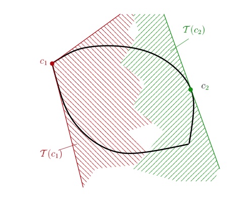
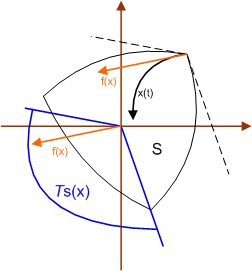
Figure 1: Tangent Cone (left) and Nagumo Theorem (right).

The following classic result proposed by Nagumo [41] provides a general criterion to determine whether a closed convex set is an invariant set for a continuous system. This theorem, however, is not valid for discrete systems, for which one can find a counterexample in [10].

Theorem 2.7.

(Nagumo [10, 41]) Let $\mathcal{S}\subseteq\mathbb{R}^{n}$ be a closed convex set, and assume that the system $\dot{x}(t)=f(x(t))$, where $f:\mathbb{R}^{n}\rightarrow\mathbb{R}^{m}$ is a continuous mapping, admits a globally unique solution for every initial point $x(0)\in\mathcal{S}$. Then $\mathcal{S}$ is an invariant set for this system if and only if

$$f(x)\in\mathcal{T}_{\mathcal{S}}(x),\text{ for all }x\in\partial\mathcal{S},$$ (10)

where $\mathcal{T}_{\mathcal{S}}(x)$ is the tangent cone of $\mathcal{S}$ at $x.$

Nagumo’s Theorem 2.7 has an intuitive geometrical interpretation as follows: for any trajectory that starts in $\mathcal{S}$, it has to go through $\partial\mathcal{S}$ if it goes out of $\mathcal{S}$. Then one needs only to consider the property of this trajectory on $\partial\mathcal{S}$. Note that $f(x)$ is the derivative of the trajectory, thus (10) ensures that the trajectory will point inside $\mathcal{S}$ on the boundary, which means $\mathcal{S}$ is an invariant set. The disadvantage of Theorem 2.7, however, is that it may be difficult to verify whether (10) holds for all points on the boundary of a given set. According to Nagumo’s Theorem 2.7, the key is to derive the formula of the tangent cone on the boundary of the set. An intuitive interpretation is given in the right side subfigure of Figure 1.

We use Euler methods to discretize continuous system (2) to derive a discrete system, because for sufficiently small step size they preserve the invariance of a set, i.e., a set, which is an invariant set for a continuous system, is also an invariant set for the corresponding derived discrete system. Here we formally present these results as follows. The first statement can be found in [8, 10, 11, 34], and the second statement can be found in [34].

Theorem 2.8.

Assume a polyhedron $\mathcal{P}$, polyhedral cone $\mathcal{C_{P}}$, ellipsoid $\mathcal{E}$ or Lorenz cone $\mathcal{C_{L}}$ is an invariant set for the continuous system (2). Then

• there exists a $\hat{\tau}>0$, such that $\mathcal{P}$ (or $\mathcal{C_{P}}$) is also an invariant set for the discrete system $x_{k+1}=(I+A\Delta t)x_{k}$ for all $0\leq\Delta t\leq\hat{\tau}$, and

• there exists a $\tilde{\tau}>0$, such that $\mathcal{P}$ ($\mathcal{C_{P}},\mathcal{E}$ or $\mathcal{C_{L}}$) is also an invariant set for the discrete system $x_{k+1}=(I-A\Delta t)^{-1}x_{k}$ for all $0\leq\Delta t\leq\tilde{\tau}$.

Remark 2.9.

The first statement in Theorem 2.8 means that the forward Euler method preserves the invariance of polyhedral set, while the second statement means that the backward Euler method preserves the invariance of polyhedral set, ellipsoid, and Lorenz cone.

3 Invariance Conditions

In this section, we present the invariance conditions, i.e., sufficient and necessary conditions under which polyhedral sets, ellipsoids, and Lorenz cones are invariant sets for discrete and continuous systems. For each convex set, the invariance conditions for discrete systems are first derived by using the Theorems of Alternatives, i.e., the Farkas lemma or the $S$-lemma. Then the invariance conditions for continuous systems are derived by using a discretization method to discretize the continuous system and applying the invariance conditions for the obtained discrete systems.

3.1 Polyhedral Sets

Since every polyhedral set has two different representations as shown in Section 2.2, we present the invariance conditions for both forms, respectively. Nonnegative and essentially nonnegative matrices are used in the invariance conditions.

Definition 3.1.

A matrix $H$ is called a nonnegative matrix, denoted by $H\geq 0$, if $H_{ij}\geq 0$ for all $i,j$. A matrix $L$ is called an essentially nonnegative matrix, denoted by $L{\geq}_{o}0$, if $L_{ij}\geq 0$ for $i\neq j$.

3.1.1 Invariance Conditions for Discrete Systems

The invariance condition of a polyhedral sets given as in (3) for a discrete system is presented in Theorem 3.2. The study of invariance condition of polyhedral sets for discrete system can be traced back to Bitsoris in [6, 7], which consider a special class of polyhedral sets that is symmetric with respect to the origin. We give a more straightforward proof here by using the Farkas lemma for the polyhedral set in the form of (3). It was brought to our attention recently that the result is the same as the one presented by Hennet [28], which also uses the Farkas lemma. To keep the integration of the paper, we also present the proof explicitly.

Theorem 3.2.

(Hennet [28]) A polyhedron $\mathcal{P}$ given as in (3) is an invariant set for the discrete system (1) if and only if there exists a matrix $H\in\mathbb{R}^{m\times m}$, such that $H\geq 0,HG=GB_{k}$ and $Hb\leq b.$

Proof.

We have that $\mathcal{P}$ is an invariant set for the discrete system (1) if and only if $B_{k}\mathcal{P}\subseteq\mathcal{P},$ which is the same as $\mathcal{P}\subseteq\mathcal{P}^{\prime}=\{x\;|\;GB_{k}x\leq b\}.$ Note that $\mathcal{P}\subseteq\mathcal{P}^{\prime}$ if and only if for every $i\in\mathcal{I}(m)$, we have

$$\{x\,|\,Gx\leq b\}\cap\{x\,|\,(GB_{k})_{i}^{T}x>b_{i}\}=\emptyset,$$

i.e., the inequality system $Gx\leq b$ and $(GB_{k})_{i}^{T}x>b_{i}$ has no solution. According to the Farkas lemma 2.4, this is equivalent to that there exists a vector $h_{i}\geq 0$, such that $G^{T}h_{i}=(GB_{k})_{i},$ and $b^{T}h_{i}\leq b_{i}.$ We let $H=[h_{1},h_{2},...,h_{m}],$ then we have $H\geq 0,HG=GB_{k}$ and $Hb\leq b$. The proof is complete. ∎

We highlight that Castelan and Hennet [16] present an algebraic characterization of the matrix $G$ satisfying the conditions in Theorem 3.2. They prove that given $B_{k}$ and $G$, there exists a matrix $H$ satisfying $HG=GB_{k}$ if and only if the kernel of $G$ is an $B_{k}$-invariant subspace.

The invariance condition of a polyhedral set given as in (4) for discrete systems is provided in Theorem 3.3. Note that a similar result is presented in [10], which considers only the case when the set is a polytope. Invariance condition of a polytope is presented in [10], while invariance condition of a polyhedral cone is presented in [54]. Here we integrate these two results in one theorem.

Theorem 3.3.

A polyhedron $\mathcal{P}$ given as in (4) is an invariant set for the discrete system (1) if and only if there exists a matrix $L\in\mathbb{R}^{(\ell_{1}+\ell_{2})\times(\ell_{1}+\ell_{2})}$, such that $L\geq 0,XL=B_{k}X$ and $\bar{1}^{T}L=\bar{1}^{T},$ where $X=[x^{1},...,x^{\ell_{1}},\hat{x}^{1},...,\hat{x}^{\ell_{2}}]$, $\bar{1}^{T}=(1_{\ell_{1}}^{T},0_{\ell_{2}}^{T})$.

Proof.

Note that $\mathcal{P}$ given as in (4) is an invariant set for the discrete system if and only if $B_{k}x^{i}\in\mathcal{P},$ for all $i\in\mathcal{I}(\ell_{1})$, and $B_{k}(O^{+}\mathcal{P})\subseteq O^{+}\mathcal{P}$, where $O^{+}\mathcal{P}$ denotes the recession cone of $\mathcal{P}$. Clearly, $B_{k}x^{i}\in\mathcal{P}$ for all $i\in\mathcal{I}(\ell_{1})$ is equivalent to that there exist ${\theta}_{p_{1}}^{i},\hat{\theta}_{p_{2}}^{i}\geq 0$, $p_{1}\in\mathcal{I}(\ell_{1}),p_{2}\in\mathcal{I}(\ell_{2}),$ with $\sum_{p_{1}=1}^{\ell_{1}}\theta_{p_{1}}^{i}=1$, such that $B_{k}x^{i}=\sum_{p_{1}=1}^{\ell_{1}}\theta_{p_{1}}^{i}x^{p_{1}}+\sum_{p_{2}=1}^{\ell_{2}}\hat{\theta}_{p_{2}}^{i}\hat{x}^{p_{2}}.$ Since $O^{+}\mathcal{P}$ is generated by $\hat{x}^{j}$, where $j\in\mathcal{I}(\ell_{2})$, we have that $B_{k}(O^{+}\mathcal{P})\subseteq O^{+}\mathcal{P}$ can be rewritten as $B_{k}\hat{x}^{j}\in O^{+}\mathcal{P},$ for all $j\in\mathcal{I}(\ell_{2})$. Then $B_{k}(O^{+}\mathcal{P})\subseteq O^{+}\mathcal{P}$ is equivalent to that there exist ${\theta}_{p_{2}}^{j}\geq 0,p_{2}\in\mathcal{I}(\ell_{2}),$ such that $B_{k}\hat{x}^{j}=\sum_{p_{2}=1}^{\ell_{2}}\hat{\theta}_{p_{2}}^{j}\hat{x}^{p_{2}}.$ Let $L=[\theta^{1},..,.\theta^{\ell_{1}},\hat{\theta}^{1},...,\hat{\theta}^{\ell_{2}}]$, then the theorem is immediate. ∎

A polyhedral cone is a special polyhedral set, thus we have the following invariance condition of a polyhedral cone for discrete systems.

Corollary 3.4.

1). A polyhedral cone $\mathcal{C_{P}}$ given as in (5) is an invariant set for the discrete system (1) if and only if there exists a matrix $H\in\mathbb{R}^{m\times m}$, such that $H\geq 0$ and $HG=GB_{k}$.

2). A polyhedral cone $\mathcal{C_{P}}$ given as in (6) is an invariant set for the discrete system (1) if and only if there exists a matrix $L\in\mathbb{R}^{\ell\times\ell}$, such that $L\geq 0$ and $XL=B_{k}X$, where $X=[\hat{x}^{1},...,\hat{x}^{\ell}]$.

For a given polyhedral set and a discrete system, according to Theorem 3.2 (Theorem 3.3, or Corollary 3.4), to determine whether the set is an invariant set for the system is equivalent to verify the existence of a nonnegative matrix $H$ (or $L$), which is actually a linear optimization problem. Rather than computing $H$ (or $L$) directly, it is more efficient to sequentially solve some small subproblems. Let us choose polyhedron $\mathcal{P}$ as given in (3) and Theorem 3.2 as an example to illustrate this idea. We can sequentially examine the feasibility of the subproblems. Find $h_{i}\in\mathbb{R}^{n}$, such that $h_{i}^{T}G=G_{i}^{T}B_{k},\,h_{i}\geq 0,$ and $h_{i}^{T}b\leq b_{i}$, for all $i\in\mathcal{I}(n)$. Clearly, these are linear feasibility problems which can be considered as a special case of linear optimization problems, see, e.g., [29]. A linear optimization problem can be solved in polynomial time, e.g., by using interior point methods [44]. If all of these linear optimization problems are feasible, then their solutions forms such a nonnegative matrix $H$. Otherwise, we can conclude that the set is not an invariant set for the system, and the computation is terminated at the first infeasible subproblem.

3.1.2 Invariance Conditions for Continuous Systems

According to [34], we have that both the forward and backward Euler methods are invariance preserving for a polyhedral set. Blanchini [8, 10] presents the connection between invariant sets for continuous and discrete systems by using the forward Euler method. The discrete system obtained by using the forward Euler method is refereed to as Euler Approximating System [8, 10]. We first present the following invariance condition which is obtained by using Nagumo’s Theorem 2.7. For $x\in\mathcal{P},$ let $\mathcal{I}_{x}$ denote the set of indices of the constraints which are active at $x$, i.e., the corresponding linear inequality holds as equality at $x$. Clearly, we have $x\in\partial\mathcal{P}$ if and only if $\mathcal{I}_{x}\neq\emptyset.$

Lemma 3.5.

Let a polyhedron $\mathcal{P}$ be given as in (3), and $\mathcal{I}_{x}\neq\emptyset$ for all $x\in\mathcal{P}$. Then $\mathcal{P}$ is an invariant set for the continuous system (2) if and only if for every $x\in\partial{\mathcal{P}}$, i.e., $G_{i}^{T}x=b_{i}$, we have

$$G_{i}^{T}Ax\leq 0,~{}~{}~{}\text{ for all }i\in\mathcal{I}_{x}.$$ (11)

Proof.

For all $x\in\partial\mathcal{P}$, the tangent cone at $x$ is $\mathcal{T}_{\mathcal{P}}(x)=\{y\,|\,G_{i}^{T}y\leq 0,i\in\mathcal{I}_{x}\}$ for all $i\in\mathcal{I}_{x}$ (see [30, p.138]). Then the lemma immediately follows from Nagumo’s Theorem 2.7. ∎

We now present another invariance condition of a polyhedron in the form of (3) for the continuous system (2). The following theorem also refers to Castelan and Hennet [16, Proposition 1].

Theorem 3.6.

A polyhedron $\mathcal{P}$ given as in (3) is an invariant set for the continuous system (2) if and only if there exists a matrix $\tilde{H}\in\mathbb{R}^{m\times m}$, such that $\tilde{H}\geq_{o}0,\tilde{H}G=GA$ and $\tilde{H}b\leq 0.$

Proof.

We first consider the “if” part. Noting that $\tilde{H}G=GA$, we have $\tilde{H}_{i}^{T}Gx=G_{i}^{T}Ax,$ for every $i\in\mathcal{I}(n)$. Since $\tilde{H}{\geq}_{o}0$ and $x\in\partial\mathcal{P}$,

$$\begin{array}[]{rl}\text{when }j=i,&\text{we have }\tilde{h}_{ii}\in\mathbb{R}\text{ and }G_{i}^{T}x=b_{i},\\ \text{when }j\neq i,&\text{we have }\tilde{h}_{ij}\geq 0\text{ and }G_{j}^{T}x\leq b_{j},\end{array}$$ (12)

where $\tilde{h}_{ij}$ is the $(i,j)$-th entry of $\tilde{H}.$ According to (12), we have $\sum_{j=1}^{m}\tilde{h}_{ij}(G_{j}^{T}x-b_{j})\leq 0,$ i.e., $\tilde{H}_{i}^{T}Gx\leq\tilde{H}_{i}^{T}b$. Since $\tilde{H}b\leq 0,$ we have $\tilde{H}_{i}^{T}b\leq 0.$ Then, we have $G_{i}^{T}Ax=\tilde{H}_{i}^{T}Gx\leq\tilde{H}_{i}^{T}b\leq 0.$ According to Lemma 3.5, we have that $\mathcal{P}$ is an invariant set for the continuous system.

Now we consider the “only if” part. According to Theorem 2.8, we have that there exists a $\hat{\tau}>0$, such that $\mathcal{P}$ is also an invariant set for the discrete system $x_{k+1}=(I+A\Delta t)x_{k},$ for every $0\leq\Delta t\leq\hat{\tau}.$ Then, according to Theorem 3.2, there exists a matrix $H(\Delta t)\geq 0$, such that $H(\Delta t)G=G(I+A\Delta t),\text{ and }H(\Delta t)b\leq b$, i.e.,

$$\frac{H(\Delta t)-I}{\Delta t}G=GA,\text{ and }\frac{H(\Delta t)-I}{\Delta t}b\leq 0.$$ (13)

Clearly $\tilde{H}=\frac{H(\Delta t)-I}{\Delta t}$ for $\Delta t>0$ satisfies this theorem. ∎

We consider the invariance condition of the polyhedron in the form of (4) for the continuous system (2). For an arbitrary convex set in $\mathbb{R}^{n}$, we have the following conclusion.

Lemma 3.7.

Let $\mathcal{S}$ be a convex set in $\mathbb{R}^{n}$. For any $\ell\in\mathbb{N}$ and $x,y^{1},y^{2},...,y^{\ell}\in\mathcal{S}$ satisfying $x=\sum_{i=1}^{\ell}\beta_{i}y^{i},$ where $\sum_{i=1}^{\ell}\beta_{i}=1$ and $\beta_{i}>0$ for every $i\in\mathcal{I}(\ell),$ we have $\mathcal{T}_{\mathcal{S}}(y^{i})\subseteq\mathcal{T}_{\mathcal{S}}(x)$ for every $i\in\mathcal{I}(\ell).$

Proof.

We denote cone$(x,\mathcal{S})=\{\alpha(y-x)\,|\,y\in\mathcal{S},\alpha\geq 0\}$, then we have that $\mathcal{T_{S}}(x)$ is the same as the topological closure of cone$(x,S)$. Let $\Phi(x)$ denote the face of $\mathcal{S}$ generated by $x$, i.e., the set $\{y\in\mathcal{S}\,|\,\mu x+(1-\mu)y\in\mathcal{S}\text{ for some }\mu>1\}.$ We first show that for any $x,u\in\mathcal{S}$, if $u\in\Phi(x)$, then $\mathcal{T_{S}}(u)\subseteq\mathcal{T_{S}}(x)$. In fact, by definition of $\Phi(x)$ there exists $\mu>1$, such that $v:=\mu x+(1-\mu)u\in\mathcal{S}.$ Then we have $x=(1-\alpha)u+\alpha v$ for some $\alpha,0<\alpha<1.$ Note that for any $y\in\mathcal{S}$, we have $(1-\alpha)y+\alpha v\in\mathcal{S}$ and $[(1-\alpha)y+\alpha v]-x=(1-\alpha)(y-u).$ It follows that cone$(u,\mathcal{S})\subseteq$cone$(x,\mathcal{S})$. By taking the closure of both sides, we have $\mathcal{T_{S}}(u)\subseteq\mathcal{T_{S}}(x)$. Since $\sum_{i=1}^{\ell}\beta_{i}=1$ and $\beta_{i}>0$ for every $i\in\mathcal{I}(\ell)$, $y^{i}\in\Phi(x)$, for every $i\in\mathcal{I}(\ell)$ we have $y^{i}\in\Phi(x)$, the lemma follows immediately. ∎

For the polyhedron $\mathcal{P}$ given as in (4), a vertex of $\mathcal{P}$ is given as $x^{i},$ for some $i\in\mathcal{I}(\ell_{1})$, and an extreme ray of $\mathcal{P}$ is represented as $x^{i}+\alpha\hat{x}^{j},\alpha>0,$ for some $i\in\mathcal{I}(\ell_{1})$ and $j\in\mathcal{I}(\ell_{2}).$ Applying Lemma 3.7 to $\mathcal{P}$, we have the following Corollary 3.8 about the relationship between tangent cones at a vector and the vertices and extreme rays of $\mathcal{P}$. Note that $\mathcal{T_{P}}(x)=\mathbb{R}^{n}$ for every $x\in\text{int}(\mathcal{S})$, thus Corollary 3.8 is only nontrivial for $x\in\partial\mathcal{P}.$

Corollary 3.8.

Let a polyhedron $\mathcal{P}$ be given as in (4), and $x\in\mathcal{P}$ be a point in $\mathcal{P}$ given as in formula (4). Let $\mathcal{I}_{1}=\{i\in\mathcal{I}(\ell_{1})\,|\,\theta_{i}>0\}$ and $\mathcal{I}_{2}=\{j\in\mathcal{I}(\ell_{2})\,|\,\hat{\theta}_{j}>0\}$. Then $\mathcal{T_{P}}(x^{i})\subseteq\mathcal{T_{P}}(x)$ and $\mathcal{T_{P}}(x^{i}+\alpha\hat{x}^{j})=\mathcal{T_{P}}(x^{i}+\hat{x}^{j})\subseteq\mathcal{T_{P}}(x)$ for $i\in\mathcal{I}_{1},j\in\mathcal{I}_{2}$, and $\alpha>0$, where $x^{i}+\alpha\hat{x}^{j}$ is an extreme ray of $\mathcal{P}$.

Let us consider a polytope $\mathcal{\tilde{P}}$ generated by $\{x^{1},x^{2},...,x^{\ell_{1}}\}$ as its vertices. Then, according to [8], we have that $\mathcal{T_{\mathcal{\tilde{P}}}}(x^{i})$ can be generated as a conic combination of $x^{p}-x^{i}$ for all $p\in\mathcal{I}(\ell_{1})$, i.e., $\mathcal{T_{\mathcal{\tilde{P}}}}(x^{i})=\{y|y=\sum_{p=1,p\neq i}^{\ell_{1}}\alpha_{p}(x^{p}-x^{i}),\alpha_{p}\geq 0\}.$ Let $\alpha_{i}=\sum_{p=1,p\neq i}^{\ell_{1}}\alpha_{p}.$ Then we have

$$\mathcal{T_{\mathcal{\tilde{P}}}}(x^{i})=\Big{\{}y|y=\sum_{p=1}^{\ell_{1}}\alpha_{p}x^{p},\alpha_{p}\geq 0,p\neq i,\sum_{p=1}^{\ell_{1}}\alpha_{p}=0\Big{\}}.$$

By a similar argument, we have that the exact representations of the tangent cones at vertices or extreme rays of $\mathcal{P}$ given as in (4) are presented in Lemma 3.9 below.

Lemma 3.9.

Let a polyhedron $\mathcal{P}$ be given as in (4), and $\mathcal{I}_{1}^{\prime}=\{i\in\mathcal{I}(\ell_{1})\,|\,$ for any $j\in\mathcal{I}(\ell_{2}),x^{i}+\hat{x}^{j}\text{ is not an extreme ray.}\}$, $\mathcal{I}_{1}^{\prime\prime}=\mathcal{I}(\ell_{1})\backslash\mathcal{I}_{1}^{\prime},$ then

1). For every $i\in\mathcal{I}_{1}^{\prime},$ we have $\mathcal{T}_{\mathcal{P}}(x^{i})=\{y\in\mathbb{R}^{n}\,|\,y=\sum_{p=1}^{\ell_{1}}\alpha_{p}x^{p},\alpha_{p}\geq 0,p\neq i,\sum_{p=1}^{\ell_{1}}\alpha_{p}=0\}.$

2). For every $i\in\mathcal{I}_{1}^{\prime\prime},$ we have $\mathcal{T}_{\mathcal{P}}(x^{i})=\{y\in\mathbb{R}^{n}\,|\,y=\sum_{p=1}^{\ell_{1}}\alpha_{p}x^{p}+\sum_{q=1}^{\ell_{2}}\hat{\alpha}_{q}\hat{x}^{q},\alpha_{p},\hat{\alpha}_{q}\geq 0,p\neq i,\sum_{p=1}^{\ell_{1}}\alpha_{p}=0\}.$

3). For every $i\in\mathcal{I}_{1}^{\prime\prime}$ and $j\in\mathcal{I}(\ell_{2})$ such that $x^{i}+\hat{x}^{j}$ is an extreme ray, we have $\mathcal{T}_{\mathcal{P}}(x^{i}+\hat{x}^{j})=\{y\in\mathbb{R}^{n}\,|\,y=\sum_{q=1}^{\ell_{2}}\hat{\alpha}_{q}\hat{x}^{q},\hat{\alpha}_{q}\geq 0,j\neq q\}.$

Lemma 3.10.

Let $\mathcal{C}$ be a closed convex cone. If $x+\alpha y\in\mathcal{C}$ for all $\alpha>0,$ then $x,y\in\mathcal{C}.$

The following lemma presents an invariance condition for a polyhedron in the form of (4) for the continuous system (2).

Lemma 3.11.

Let a polyhedron $\mathcal{P}$ be given as in (4). Then $\mathcal{P}$ is an invariant set for the continuous system (2) if and only if $Ax^{i}\in\mathcal{T}_{\mathcal{P}}(x^{i})$ and $A\hat{x}^{j}\in\mathcal{T}_{\mathcal{P}}(x^{i}+\hat{x}^{j})$ for $i\in\mathcal{I}(\ell_{1})$ and $j\in\mathcal{I}(\ell_{2})$, where $x^{i}+\alpha\hat{x}^{j}$ for $\alpha\geq 0$ is an extreme ray of $\mathcal{P}.$

Proof.

We first consider the “only if” part. According to Nagumo’s Theorem 2.7, for any $i\in\mathcal{I}(\ell_{1})$ and $j\in\mathcal{I}(\ell_{2})$ when $x^{i}+\alpha\hat{x}^{j}$ for $\alpha\geq 0$ is an extreme ray, we have $Ax^{i}\in\mathcal{T}_{\mathcal{P}}(x^{i})$ and $A(x^{i}+\alpha\hat{x}^{j})\in\mathcal{T}_{\mathcal{P}}(x^{i}+\hat{x}^{j})$. By Lemma 3.10, this implies that $A\hat{x}^{j}\in\mathcal{T}_{\mathcal{P}}(x^{i}+\hat{x}^{j})$.

For the “if” part, we choose $x\in\mathcal{P}.$ We represent $x$ as $x=\sum_{i\in\mathcal{I}_{1}}\theta_{i}x^{i}+\sum_{j\in\mathcal{I}_{2}}\hat{\theta}_{j}\hat{x}^{j},$ where $\mathcal{I}_{1}=\{i\in\mathcal{I}(\ell_{1})\,|\,\theta_{i}>0\}$ and $\mathcal{I}_{2}=\{j\in\mathcal{I}(\ell_{2})\,|\,\hat{\theta}_{j}>0\}.$ Then according to Corollary 3.8, we have $Ax=\sum_{i\in\mathcal{I}_{1}}\theta_{i}Ax^{i}+\sum_{j\in\mathcal{I}_{2}}\hat{\theta}_{j}A\hat{x}^{j}$. Note that $Ax^{i}\in\mathcal{T}_{\mathcal{P}}(x^{i})\subseteq\mathcal{T}_{\mathcal{P}}(x)$ and $A\hat{x}^{j}\in\mathcal{T}_{\mathcal{P}}(x^{i}+\hat{x}^{j})\subseteq\mathcal{T}_{\mathcal{P}}(x)$. Since $\mathcal{T}_{\mathcal{P}}$ is a convex cone, it is closed under vector addition. So we have $Ax\in\mathcal{T}_{\mathcal{P}}(x).$ Finally, the “if” part follows by Nagumo’s Theorem 2.7. ∎

By Lemma 3.9 and Lemma 3.11, the following corollary is immediate.

Corollary 3.12.

Let a polyhedron $\mathcal{P}$ be given as in (4). Then $\mathcal{P}$ is an invariant set for the continuous system (2) if and only if for $x^{i}$, $i\in\mathcal{I}(\ell_{1})$, there exist $\alpha_{p}^{i},\hat{\alpha}_{q}^{i}\geq 0$ for $p\neq i$, $\alpha_{i}^{i}\leq 0$, such that

$$Ax^{i}=\sum_{p=1}^{\ell_{1}}\alpha_{p}^{i}x^{p}+\sum_{q=1}^{\ell_{2}}\hat{\alpha}_{q}^{i}\hat{x}^{q},\text{ and }\sum_{p=1}^{\ell_{1}}\alpha_{p}^{i}=0,$$ (14)

for $\hat{x}^{j}$, $j\in\mathcal{I}(\ell_{2})$, there exist $\hat{\alpha}_{q}^{j}\geq 0$ for $q\neq j$, and $\hat{\alpha}_{j}^{j}\in\mathbb{R},$ such that $A\hat{x}^{j}=\sum_{q=1}^{\ell_{2}}\hat{\alpha}_{q}^{j}\hat{x}^{q}.$

Theorem 3.13.

A polyhedron $\mathcal{P}$ given as in (4) is an invariant set for the continuous system (2) if and only if there exists a matrix $\tilde{L}\in\mathbb{R}^{(\ell_{1}+\ell_{2})\times(\ell_{1}+\ell_{2})}$, such that $\tilde{L}{\geq}_{o}0$, $X\tilde{L}=AX$, and $\bar{1}\tilde{L}=\bar{0},$ where $X=[x^{1},...,x^{\ell_{1}},\hat{x}^{1},...,\hat{x}^{\ell_{2}}]$, $\bar{1}=[1_{\ell_{1}},0_{\ell_{2}}].$

Proof.

This proof is similar to the one given in Theorem 3.6. We denote the $i$-th column of $\tilde{L}$ by $(l_{1,i},...,l_{\ell_{1}+\ell_{2},i})^{T}$.

For the “if” part, we consider $x^{i}$ with $i\in\mathcal{I}(\ell_{1})$. Since $\tilde{L}{\geq}_{o}0$, $X\tilde{L}=AX$, and $\bar{1}\tilde{L}=\bar{0}$, we have $Ax^{i}=\sum_{p=1}^{\ell_{1}}l_{p,i}x^{i}+\sum_{q=1}^{\ell_{2}}l_{\ell_{1}+q,i}\hat{x}^{q},\text{ with }\sum_{p=1}^{\ell_{1}}l_{p,i}=0,\text{ and }l_{p,i}\geq 0,\text{ for }p\neq i.$ The argument for $\hat{x}^{j}$ with $j\in\mathcal{I}(\ell_{2})$ is similar. Then, according to Corollary 3.12, we have that $\mathcal{P}$ is an invariant set for the continuous system.

For the “only if” part, the proof is similar to the one in Theorem 3.6. According to Theorem 2.8 and Theorem 3.3, we know that there exists a nonnegative matrix $L(\Delta t)$ and a scalar $\hat{\tau}>0$, such that $XL(\Delta t)=(I+\Delta tA)X,~{}~{}\bar{1}L(\Delta t)=\bar{1},\text{ for }0\leq\Delta t\leq\hat{\tau},$ i.e.,

$$X\frac{L(\Delta t)-I}{\Delta t}=AX,~{}~{}\bar{1}\frac{L(\Delta t)-I}{\Delta t}=\bar{0}.$$

Let $\tilde{L}=\frac{L(\Delta t)-I}{\Delta t}$, the theorem is immediate. ∎

Since the invariance conditions for a polyhedral cone given in the two different forms can be obtained by similar discussions as above, we only present these invariance conditions without providing the proofs.

Corollary 3.14.

1). A polyhedral cone $\mathcal{C_{P}}$ given as in (5) is an invariant set for the continuous system (2) if and only if there exists a matrix $\tilde{H}\in\mathbb{R}^{m\times m}$, such that $\tilde{H}\geq_{o}0$ and $\tilde{H}G=GA$.

2).A polyhedral cone $\mathcal{C_{P}}$ given as in (6) is an invariant set for the continuous system (2) if and only if there exists a matrix $\tilde{L}\in\mathbb{R}^{\ell\times\ell}$, such that $\tilde{L}\geq_{o}0$ and $X\tilde{L}=AX$, where $X=[\hat{x}^{1},...,\hat{x}^{\ell}]$.

According to Theorem 3.13 and Corollary 3.14, verifying if a polyhedron given as in (4) or polyhedral cone given as in (6) is an invariant set for the continuous system (2) can be done by solving a series of linear optimization problems.

3.2 Ellipsoids

In this section, we consider the invariance condition for ellipsoids which are represented by a quadratic inequality.

3.2.1 Invariance Conditions for Discrete Systems

The S-lemma and Proposition 2.3 are our main tools to obtain the invariance condition of an ellipsoid for a discrete system. First, we present a technical lemma.

Lemma 3.15.

Let $Q$ be an $n\times n$ real symmetric matrix and let $\alpha$ be a given real number. Then $x^{T}Qx\geq\alpha$ for all $x\in\mathbb{R}^{n}$ if and only if $Q\succeq 0$, and $\alpha\leq 0.$

Theorem 3.16.

An ellipsoid $\mathcal{E}$ given as in (7) is an invariant set for the discrete system (1) if and only if

$$\exists\,\mu\in[0,1],\text{ such that }B_{k}^{T}QB_{k}-\mu Q\preceq 0.$$ (15)

Proof.

According to Proposition 2.3, to prove this theorem is equivalent to prove $\mathcal{E}\subseteq\mathcal{E}^{\prime}$, where $\mathcal{E}=\{x\,|\,x^{T}Qx\leq 1\}$ and $\mathcal{E}^{\prime}=\{x\,|\,x^{T}B_{k}^{T}QB_{k}x\leq 1\}.$ Clearly, $\mathcal{E}\subseteq\mathcal{E}^{\prime}$ holds if and only if the following inequality system has no solution:

$$-x^{T}B_{k}^{T}QB_{k}x+1<0,~{}~{}x^{T}Qx-1\leq 0.$$ (16)

Note that the left sides of the two inequalities in (16) are both quadratic functions, thus, according to the S-lemma, we have that (16) has no solution is equivalent to that there exists $\mu\geq 0$, such that $-x^{T}B_{k}^{T}QB_{k}x+1+\mu(x^{T}Qx-1)\geq 0,$ or equivalently,

$$x^{T}(\mu Q-B_{k}^{T}QB_{k})x\geq\mu-1,~{}~{}\text{ for all }x\in\mathbb{R}^{n}.$$ (17)

The theorem follows by applying Lemma 3.15 to (17). ∎

We can also consider an ellipsoid as an invariant set for a system in the following perspective. Invariance of a bounded set for a system is possible only if the system is non-expansive, which means that for discrete system (1), all eigenvalues of $B_{k}$ are in a closed unit disc of the complex plane. Then it becomes clear that (15) has a solution only if (1) is non-expansive, i.e., the trajectory of (1) is non-expansive. One can conclude from this that there is an invariant ellipsoid for (1) if and only if (15) has a solution for a positive definite $Q$.

Moreover, we can also observe that the smallest $\mu$ solving (15) is the largest eigenvalue of $WA^{T}QAW$, where $W$ is the symmetric positive definite square root of $Q^{-1}$, i.e., $W^{2}=Q^{-1}.$

We now present two examples such that condition (15) does not hold for $\mu\not\in[0,1]$. First, let $Q$ be positive definite and $\mu<0$, then $B_{k}^{T}QB_{k}-\mu Q$ is always a positive definite matrix. Thus condition (15) does not hold. Second, let $Q$ be positive definite and $\mu>1$, consider the discrete system $x_{k+1}=-x_{k}.$ One can prove that $\{x\,|\,x^{T}Qx\leq 1\}$ is an invariant set for this discrete system. However, in this case, we have $B_{k}^{T}QB_{k}-\mu Q=(1-\mu)Q$, which is always a negative definite matrix. Thus condition (15) does not hold either.

Apart from the simplicity, another advantage of the approach given in the proof of Theorem 3.16 is that it obtains a sufficient and necessary condition. Also, this approach highlights the close relationship between the theory of invariant sets and the Theorem of Alternatives, which is a fundamental result in optimization community.

Corollary 3.17.

Condition (15) holds if and only if

$$\exists\,\nu\in[0,1],\text{ such that }\tilde{Q}=\left(\begin{array}[]{cc}Q^{-1}&B_{k}\\ B_{k}^{T}&\nu Q\\ \end{array}\right)\succeq 0.$$ (18)

Proof.

First, $Q\succ 0$ yields $Q^{-1}\succ 0$. By Schur’s lemma [15], $\tilde{Q}\succeq 0$ if and only if its Schur complement $\nu Q-B_{k}^{T}(Q^{-1})^{-1}B_{k}=\nu Q-B_{k}^{T}QB_{k}\succeq 0$, i.e., (15) holds. ∎

Corollary 3.18.

Condition (15) holds if and only if

$$B_{k}^{T}QB_{k}-Q\preceq 0.$$ (19)

Proof.

The “if” part is immediate by letting $\mu=1$ in (15). For the “only if” part, we let $\nu=1-\mu$, which, by reformulating (15), yields $B_{k}^{T}QB_{k}-Q\preceq-\nu Q\preceq 0,\text{ for }\nu\in[0,1],$ where the second $``\preceq$” holds due to the fact that $\nu\geq 0$ and $Q\succ 0$. ∎

The left side of (19) is called the Lyapunov operator [14] in discrete form or Stein transformation [48] in dynamical system. Corollary 3.18 is consistent with the invariance condition of an ellipsoid for discrete system given in [10, 14]. The invariance condition presented in [10] is the same as (19) without the equality. This is since contractivity rather than invariance of a set for a system is analyzed in [10]. Lyapunov method is used to derive condition (19) in [14]. Apparently, condition (19) is easier to apply than condition (15), since the former one involves only about the ellipsoid and the system.

The attentive reader may observe that the positive definiteness assumption for matrix Q is never used in the proof of Theorem 3.16. That assumption was only needed to ensure that the set $\mathcal{S}$ is convex. Recall that the quadratic functions in the S-lemma are not necessarily convex, thus we can extend Theorem 3.16 to general sets which are represented by a quadratic inequality.

Theorem 3.19.

A set $\mathcal{S}=\{x\in\mathbb{R}^{n}\,|\,x^{T}Qx\leq 1\}$, where $Q\in\mathbb{R}^{n\times n},$ is an invariant set for the discrete system (1) if and only if

$$\exists\,\mu\in[0,1],\text{ such that }B_{k}^{T}QB_{k}-\mu Q\preceq 0.$$ (20)

The proof of Theorem 3.19 is the same as that of Theorem 3.16, so we do not duplicate that proof here. A trivial example that satisfy the condition in is given by choosing $Q$ to be any indefinite matrix, $B_{k}=I$, and we choose $\mu=1$. It is easy to see that for this choice condition (24) holds. Further exploring the implications of possibly using nonconvex and unbounded invariant sets is far from the main focus of our paper, so this topic remains the subject of further research.

3.2.2 Invariance Conditions for Continuous Systems

We first present an interesting result about the solution of continuous system.

Proposition 3.20.

The solution of the continuous system (2) is on the boundary of the ellipsoid $\mathcal{E}$ given as in (7) (or the Lorenz cone $\mathcal{C_{L}}$ given as in (8)) whenever $x_{0}\in\partial\mathcal{E}$(or $x_{0}\in\partial\mathcal{C_{L}}$) if and only if

$$\sum_{i=0}^{k-1}\frac{1}{(k-1)!}\binom{k-1}{i}(A^{i})^{T}QA^{k-i-1}=0,\text{ for }k=2,3,....$$ (21)

Proof.

We consider only ellipsoids, and the proof for Lorenz cones is similar. The solution of (2) is given as $x(t)=e^{At}x_{0},$ thus $x(t)\in\partial\mathcal{E}$ if and only if $x_{0}^{T}(e^{At})^{T}Qe^{At}x_{0}=1,$ which can be expanded, by substituting $e^{At}=\sum_{i=0}^{\infty}\frac{A^{i}}{i!}t^{i}$, as

$$\sum_{k=1}^{\infty}t^{k-1}x_{0}^{T}\tilde{Q}_{k-1}x_{0}=1,\text{ where }\tilde{Q}_{k-1}=\sum_{i=0}^{k-1}\frac{1}{(i)!(k-i-1)!}(A^{i})^{T}QA^{k-i-1},$$

for any $x_{0}^{T}Qx_{0}=1$ and $t\geq 0.$ Thus, $\tilde{Q}_{k-1}=0,$ for $k\geq 2.$ Also, note that $\frac{1}{(k-1)!}\binom{k-1}{i}=\frac{1}{(i)!(k-i-1)!}$, condition (21) is immediate. ∎

In particular, when $k=2$, condition (21) yields $A^{T}Q+QA=0$. The left hand side of this equation is called Lyapunov operator in continuous form. The following invariance conditions is first given by Stern and Wolkowicz [50], where they consider only Lorenz cones and their proof is using the concept of cross-positivity. Here we present a simple proof.

Lemma 3.21.

[50] An ellipsoid $\mathcal{E}$ given in the form of (7) (or a Lorenz cone $\mathcal{C_{L}}$ given in the form of (8)) is an invariant set for the continuous system (2) if and only if

$$(Ax)^{T}Qx\leq 0,\text{ for all }x\in\partial\mathcal{E}~{}(\text{ or }x\in\partial\mathcal{C_{L}}).$$ (22)

Proof.

We consider only ellipsoids, and the proof is analogous for Lorenz cones. Note that $\partial\mathcal{E}=\{x\,|\,x^{T}Qx=1\}$, thus the outer normal vector of $\mathcal{E}$ at $x\in\partial\mathcal{E}$ is $Qx$. Then we have $\mathcal{T}_{\mathcal{E}}(x)=\{y\,|\,y^{T}Qx\leq 0\}$, thus this theorem follows by Theorem 2.7. ∎

We now present a sufficient and necessary condition that an ellipsoid is invariant for the continuous system.

Theorem 3.22.

An ellipsoid $\mathcal{E}$ given as in (7) is an invariant set for the continuous system (2) if and only if

$$A^{T}Q+QA\preceq 0.$$ (23)

Proof.

According to Lemma 3.21, we have that condition (22) holds, i.e., $\mathcal{E}$ is an invariant set for the continuous system if and only if

$$x^{T}(A^{T}Q+QA)x\leq 0,\text{ for all }x\in\partial\mathcal{E}.$$ (24)

Clearly (23) implies (24). Now assume (24) holds. Then for all nonzero $y\in\mathbb{R}^{n},$ there exists an $x\in\partial\mathcal{E}$ and $\gamma>0$, such that $y=\gamma x.$ Then $y^{T}(A^{T}Q+QA)y=\frac{1}{\gamma^{2}}x^{T}(A^{T}Q+QA)x\leq 0,$ which yields condition (23). ∎

The presented method in the proof of Theorem 3.22 is simpler than the traditional Lyapunov method to derive the invariance condition. However, the approach in the proof cannot be used for Lorenz cones, since the origin is not in the interior of Lorenz cones.

3.3 Lorenz Cones

A Lorenz cone $\mathcal{C_{L}}$ given as in (8) also has a quadratic form, but the way to obtain the invariance condition of a Lorenz cone for discrete system is much more complicated than that for an ellipsoid. The difficulty is mainly due to the existence of the second constraint in (8).

3.3.1 Invariance Conditions for Discrete Systems

The representation of the nonconvex set $\mathcal{C_{L}}\cup(-\mathcal{C_{L}})=\{x\,|\,x^{T}Qx\leq 0\}$ involves only the quadratic form, which is almost the same as an ellipsoid. We can first derive the invariance condition of this set for discrete system. Recall that the S-lemma does not require that the quadratic functions have to be convex, thus the S-lemma is still valid for the nonconvex set.

Theorem 3.23.

The nonconvex set $\mathcal{C_{L}}\cup(-\mathcal{C_{L}})$ is an invariant set for the discrete system (1) if and only if

$$\exists\,\mu\geq 0,\text{ such that }B_{k}^{T}QB_{k}-\mu Q\preceq 0.$$ (25)

Proof.

The proof is closely following the ideas in the proof of Theorem 3.16. The only difference is that the right side in (17) is 0 rather than $1-\mu$, which is why the condition $\mu\leq 1$ is absent in this case. ∎

The invariance condition for $\mathcal{C_{L}}\cup(-\mathcal{C_{L}})$ shown in (25) is similar to the one proposed by Loewy and Schneider in [38]. They proved by contradiction using the properties of copositive matrices that when the rank of $A$ is greater than 1, $B_{k}\mathcal{C_{L}}\subseteq\mathcal{C_{L}}$ or $-B_{k}\mathcal{C_{L}}\subseteq\mathcal{C_{L}}$ if and only if (25) holds. They also concluded (see [38, Lemma 3.1]) that when the rank of $B_{k}$ is 1, $B_{k}\mathcal{C_{L}}\subseteq\mathcal{C_{L}}$ if and only if there exist two vectors $x,y\in\mathcal{C_{L}}$, such that $B_{k}=xy^{T}$.

The following example shows that for the given $B_{k}$ and $Q$, only $\mu=1$ satisfies condition (25). Let $B_{k}=Q=\text{{diag}}\{1,...,1,-1\}$. Then the Lorenz cone is an invariant set for the system, since such a Lorenz cone is a self-dual cone. The left hand side in (25) is, however, now simplified to $(1-\mu)Q$ which is negative semidefinite only for $\mu=1,$ because inertia$\{Q\}=\{n-1,0,1\}$.

In the case of ellipsoids, we used Schur’s lemma, see, e.g., [44], to simplify invariance condition (15) to (18), which was further simplified to the parameter free invariance condition (19). Although conditions (15) and (25) are similar, it seems to be impossible to develop a parameter free condition analogous to (19) for Lorenz cone. This is since matrix $Q$ for a Lorenz cone is neither positive nor negative semidefinite.

To find the scalar $\mu$ in (25) is essentially a semidefinite optimization (SDO) problem. Various celebrated SDO solvers, e.g., SeDuMi [51], CVX [25], and SDPT3 [55] have been shown robust performance in solving a SDO problems numerically.

Corollary 3.24.

If $\lambda_{1}(B_{k}^{T}QB_{k})\leq 0$, then the Lorenz cone $\mathcal{C_{L}}$ given as in (8) is an invariant set for the discrete system (1).

Corollary 3.24 gives a simple sufficient condition such that a Lorenz cone is an invariant set. However, one must note that this result is valid only if matrix $B_{k}$ is singular. Let $\text{dim}(M)$ represent the dimension of a matrix $M$. In fact, if $B_{k}$ is nonsingular, then by Sylvester’s law of inertia [31], we have that $\lambda_{1}(B_{k}^{T}QB_{k})>0$. When $\lambda_{1}(B_{k}^{T}QB_{k})\leq 0$, we have that the rank of $B_{k}$ is at most 1. This is because, if the rank is larger than 1, then range$(B_{k})\cap\text{span}\{u_{1},u_{2},...,u_{n-1}\}$ must be a nonzero subspace. This is since the sum of $\text{dim}(\text{range}(B_{k}))$ and $\text{dim}(\text{span}\{u_{1},u_{2},...,u_{n-1}\})$ is greater than or equal to $2+(n-1)=n+1>n,$ and $\text{dim}(\text{range}(B_{k}))\cap\text{span}\{u_{1},u_{2},...,u_{n-1}\})$ is greater than or equal to 1. Then let $0\neq x\in$ range$(B_{k})\cap\text{span}\{u_{1},u_{2},...,u_{n-1}\}$, we have $x^{T}(B_{k}^{T}QB_{k})x>0$, which contradicts to $\lambda_{1}(B_{k}^{T}QB_{k})\leq 0.$ Also, note that the rank of $B_{k}^{T}QB_{k}$ is less than or equal to the minimum of the rank of $B_{k}$ and the rank of $Q$, so if $B_{k}^{T}QB_{k}$ is not zero matrix and $\lambda_{1}(B_{k}^{T}QB_{k})\leq 0$, then the rank of $B_{k}$ is equal to 1.

The interval of the scalar $\mu$ in (25) can be tightened by incorporating the eigenvalues and eigenvectors of $Q$. Such a tighter condition is presented in Corollary 3.25.

Corollary 3.25.

If $\mu$ satisfies $B_{k}^{T}QB_{k}-\mu Q\preceq 0$, then

$$\max\Big{\{}0,\max_{1\leq i\leq n-1}\Big{\{}\frac{u_{i}^{T}B_{k}^{T}QB_{k}u_{i}}{\lambda_{i}}\Big{\}}\Big{\}}\leq\mu\leq\frac{u_{n}^{T}B_{k}^{T}QB_{k}u_{n}}{\lambda_{n}}.$$ (26)

Proof.

Multiplying condition (25) by $u_{i}^{T}$ from the left and $u_{i}$ from the right, we have $u_{i}^{T}B_{k}^{T}QB_{k}u_{i}-\mu u_{i}^{T}Qu_{i}\leq 0$. Since $u_{i}^{T}Qu_{i}=\lambda_{i}u_{i}^{T}u_{i}=\lambda_{i}>0$, for $i\in\mathcal{I}(n-1)$, and $u_{n}^{T}Qu_{n}=\lambda_{n}<0$, condition (26) follows immediately. ∎

Corollary 3.25 presents tighter bounds for the scalar $\mu$ in (26) in terms of an algebraic form. The existence of a scalar $\mu$ implies that the upper bound should be no less than the lower bound in (26). However, this is not always true. We now present a geometrical interpretation of the interval of the scalar $\mu$, that can be directly derived from Corollary 3.25.

Corollary 3.26.

The relationship between the vector $B_{k}u_{i},$ and the scalars $u_{i}^{T}B_{k}^{T}QB_{k}u_{i}$, and $\mu$ are as follows:

• If $B_{k}u_{n}\notin\mathcal{C_{L}}\cup(-\mathcal{C_{L}})$, then $\mu$ satisfying (26) does not exist.

• If $B_{k}u_{i}\in\mathcal{C_{L}}\cup(-\mathcal{C_{L}})$ for all $i\in\mathcal{I}(n-1)$, then

  • if $B_{k}u_{n}\in\partial\mathcal{C_{L}}\cup(-\partial\mathcal{C_{L}})$ and (26) holds, then $\mu=0$.

  • if $B_{k}u_{n}\in\emph{int }\mathcal{C_{L}}\cup(-\emph{int }\mathcal{C_{L}})$ and (26) holds, then $\mu\in\Big{[}0,\frac{u_{n}^{T}B_{k}^{T}QB_{k}u_{n}}{\lambda_{n}}\Big{]}.$

• Let $\mathcal{I}=\{i\;|\;B_{k}u_{i}\notin\mathcal{C_{L}}\cup(-\mathcal{C_{L}})\}$. If the set $\mathcal{I}\subseteq\mathcal{I}(n-1)$ is nonempty, then

  • if $B_{k}u_{n}\in\partial\mathcal{C_{L}}\cup(-\partial\mathcal{C_{L}})$, then $\mu$ satisfying (26) does not exist.

  • if $B_{k}u_{n}\in\emph{int }(\mathcal{C_{L}})\cup(-\emph{int}(\mathcal{C_{L}}))$, then

    • if there exist $i^{*}\in\mathcal{I}$, such that $\frac{u_{i^{*}}^{T}B_{k}^{T}QB_{k}u_{i^{*}}}{\lambda_{i^{*}}}>\frac{u_{n}^{T}B_{k}^{T}QB_{k}u_{n}}{\lambda_{n}}$, then $\mu$ satisfying (26) does not exist.

    • otherwise, if (26) holds, then
      $\mu\in\Big{[}\max_{i\in\mathcal{I}}\Big{\{}\frac{u_{i}^{T}B_{k}^{T}QB_{k}u_{i}}{\lambda_{i}}\Big{\}},\frac{u_{n}^{T}B_{k}^{T}QB_{k}u_{n}}{\lambda_{n}}\Big{]}$.

We now consider the invariance condition of a Lorenz cone $\mathcal{C_{L}}$ given as in (8), which is a convex set and can handle expansive systems.

Lemma 3.27.

[50] A Lorenz cone $\mathcal{C_{L}}$ given as in (8) can be written as $T\mathcal{K}_{n}$, where $\mathcal{K}_{n}$ is the standard Lorenz cone and $T$ is the nonsingular matrix,

$$T=\Big{[}\frac{u_{1}}{\sqrt{\lambda_{1}}},...,\frac{u_{n-1}}{\sqrt{\lambda_{n-1}}},\frac{u_{n}}{\sqrt{-\lambda_{n}}}\Big{]}.$$ (27)

Lemma 3.28.

A Lorenz cone $\mathcal{C_{L}}$ given as in (8) is an invariant set for the discrete system (1) if and only if the standard Lorenz cone $\mathcal{K}_{n}$ is an invariant set for the following discrete system

$$x_{k+1}=T^{-1}B_{k}Tx_{k},$$ (28)

where $T$ is defined as (27).

Proof.

The Lorenz cone $\mathcal{C_{L}}$ is an invariant set for (1) if and only if $B_{k}\mathcal{C_{L}}\subseteq\mathcal{C_{L}}$. This holds if and only if $B_{k}T\mathcal{K}_{n}\subseteq T\mathcal{K}_{n}$, which is equivalent to $T^{-1}B_{k}T\mathcal{K}_{n}\subseteq\mathcal{K}_{n}$. ∎

The invariance condition of a Lorenz cone for discrete systems is presented in Theorem 3.29. Although we have developed such invariance condition independently, it was brought to our attention recently that the invariance condition is the same as the one proposed by Aliluiko and Mazko in [2]. But our proof is more straightforward.

Theorem 3.29.

A Lorenz cone $\mathcal{C_{L}}$ (or $-\mathcal{C_{L}}$) given as in (8) is an invariant set for the discrete system (1) if and only if

$$\exists\,\mu\geq 0,\text{ such that }B_{k}^{T}QB_{k}-\mu Q\preceq 0,~{}u_{n}^{T}B_{k}u_{n}\geq 0,~{}u_{n}^{T}B_{k}Q^{-1}B_{k}^{T}u_{n}\leq 0,$$ (29)

where $u_{n}$ is the eigenvector corresponding to the unique negative eigenvalue $\lambda_{n}$ of $Q.$

Proof.

Since $B_{k}\mathcal{C_{L}}\subseteq\mathcal{C_{L}}$ if and only $B_{k}(-\mathcal{C_{L}})\subseteq-\mathcal{C_{L}},$ we only present the proof for $\mathcal{C_{L}}$. For an arbitrary $x\in\mathcal{C_{L}}$, by Theorem 3.23, we have that $B_{k}x\in\mathcal{C_{L}}$ or $B_{k}x\in-\mathcal{C_{L}}$ if and only if condition (25) is satisfied. To ensure that only $B_{k}x\in\mathcal{C_{L}}$ holds, some additional conditions should be added.

According to Lemma 3.28, we may consider $\mathcal{K}_{n}$ and the discrete system (28), where the coefficient matrix, denoted by $\tilde{A}$, can be explicitly written as

$$\tilde{A}=T^{-1}B_{k}T=\left[\begin{array}[]{ccc}u_{1}^{T}B_{k}u_{1}&\cdots&\sqrt{-\frac{\lambda_{1}}{\lambda_{n}}}u_{1}^{T}B_{k}u_{n}\\ \vdots&\ddots&\vdots\\ \sqrt{-\frac{\lambda_{n}}{\lambda_{1}}}u_{n}^{T}B_{k}u_{1}&\cdots&u_{n}^{T}B_{k}u_{n}\\ \end{array}\right].$$

Then, according to Theorem 3.23, condition (25) is equivalent to

$$\exists\,\mu\geq 0,\text{ such that }(T^{-1}B_{k}T)^{T}\tilde{I}T^{-1}B_{k}T-\mu\tilde{I}\preceq 0,$$ (30)

where $\tilde{I}=\text{{diag}}\{1,...,1,-1\}$. Note that $T^{T}QT=\tilde{I}$, condition (30) is equivalent to

$$\exists\,\mu\geq 0,\text{ such that }B_{k}^{T}QB_{k}-\mu Q\preceq 0.$$

Recall that we denote the $i$-th row of a matrix $M$ by $M_{i}^{T}.$ Also, the second constraint in the formulae of $\mathcal{K}_{n}$ requires that for every $x\in\mathcal{K}_{n}$ the last coordinate in $x$ is nonnegative. Since $\tilde{A}\mathcal{K}_{n}\subseteq\mathcal{K}_{n}$, we have $\tilde{A}_{n}^{T}x\geq 0,\text{ for all }x\in\mathcal{K}_{n}.$ Note that $\mathcal{K}_{n}$ is a self-dual cone, we have $\tilde{A}_{n}^{T}x\geq 0,\text{ for all }x\in\mathcal{K}_{n}$ if and only if $\tilde{A}_{n}\in\mathcal{K}_{n}$. Now we have

$$\tilde{A}_{n}^{T}=\sqrt{-\lambda_{n}}\Big{(}\frac{1}{\sqrt{\lambda_{1}}}u_{n}^{T}B_{k}u_{1},\frac{1}{\sqrt{\lambda_{2}}}u_{n}^{T}B_{k}u_{2},...,\frac{1}{\sqrt{-\lambda_{n}}}u_{n}^{T}B_{k}u_{n}\Big{)}=\sqrt{-\lambda_{n}}u_{n}^{T}B_{k}T.$$ (31)

Substituting the value of $\tilde{A}_{n}^{T}$ given by the right side of (31) into the first inequality in the formulae of $\mathcal{K}_{n}$, we have

$$-\lambda_{n}(T^{T}B_{k}^{T}u_{n})^{T}\tilde{I}(T^{T}B_{k}^{T}u_{n})\leq 0.$$ (32)

Since $\lambda_{n}<0$ and $T\tilde{I}T^{T}=\sum_{i=1}^{n}\frac{u_{i}u_{i}^{T}}{\lambda_{i}}=Q^{-1}$, where the second equality is due to the spectral decomposition of $Q^{-1}$, we have that (32) is equivalent to $u_{n}^{T}B_{k}Q^{-1}B_{k}^{T}u_{n}\leq 0.$ Also, substituting (31) into the second inequality in the formulae of $\mathcal{K}_{n}$ yields $u_{n}^{T}B_{k}u_{n}\geq 0.$ The proof is complete. ∎

Remark 3.30.

The inequality system $u_{n}^{T}B_{k}Q^{-1}B_{k}^{T}u_{n}\leq 0$ and $u_{n}^{T}B_{k}u_{n}\geq 0$ holds if and only if $u_{n}^{T}B_{k}x\geq 0$, for all $x\in\mathcal{C_{L}}.$

Proof.

Since $x^{T}Qx\leq 0$ can be written as $x^{T}U\Lambda^{\frac{1}{2}}\tilde{I}\Lambda^{\frac{1}{2}}U^{T}x\leq 0$, we have $x\in\mathcal{C_{L}}$ if and only if $\Lambda^{\frac{1}{2}}U^{T}x\in\mathcal{K}_{n}.$ Similarly, since $Q^{-1}=U\Lambda^{-\frac{1}{2}}\tilde{I}\Lambda^{-\frac{1}{2}}U^{T},$ we have $u_{n}^{T}B_{k}Q^{-1}B_{k}^{T}u_{n}\leq 0$ can be written as $u_{n}^{T}B_{k}U\Lambda^{-\frac{1}{2}}\tilde{I}\Lambda^{-\frac{1}{2}}U^{T}B_{k}^{T}u_{n}\leq 0$, which yields $\Lambda^{-\frac{1}{2}}U^{T}B_{k}^{T}u_{n}\in\mathcal{K}_{n}\cup(-\mathcal{K}_{n}).$ Since the set $\mathcal{K}_{n}$ is a self-dual cone, we have $(\Lambda^{-\frac{1}{2}}U^{T}B_{k}^{T}u_{n})^{T}(\Lambda^{\frac{1}{2}}U^{T}x)\geq 0$, which can be simplified to $u_{n}^{T}B_{k}x\geq 0$, for all $x\in\mathcal{C_{L}}.$ ∎

The normal plane of the eigenvector $u_{n}$ that contains the origin separates $\mathbb{R}^{n}$ into two half spaces. Corollary 3.30 presents a geometrical interpretation that $A$ transforms the Lorenz cone $\mathcal{C_{L}}$ to the half space that contains eigenvector $u_{n}$, i.e., $B_{k}\mathcal{C_{L}}\subseteq\{y\,|~{}u_{n}^{T}y\geq 0\}$. Moreover, note that $u_{n}^{T}B_{k}x=(B_{k}^{T}u_{n})^{T}x,$ which shows that the vector $B_{k}^{T}u_{n}$ is in the dual cone of $\mathcal{C_{L}}.$

Corollary 3.31.

If condition (29) holds, then

$$0\leq\mu\leq\frac{u_{n}^{T}B_{k}^{T}QB_{k}u_{n}}{\lambda_{n}}.$$ (33)

Proof.

The proof is analogous to the one given in the proof of Corollary 3.25. ∎

The interval for the scalar $\mu$ in condition (33) is wider but simpler than the one presented in Corollary 3.25. Analogous to Corollary 3.26, we present an intuitive geometrical interpretation of $\mu$ for Lorenz cones.

Corollary 3.32.

The relationship between the vector $B_{k}u_{n},$ and the scalars $u_{n}^{T}B_{k}^{T}QB_{k}u_{n}$, and $\mu$ are as follows:

• If $B_{k}u_{n}\notin\mathcal{C_{L}}\cup(-\mathcal{C_{L}})$, then $\mu$ satisfying (33) does not exist.

• If $B_{k}u_{n}\in\partial\mathcal{C_{L}}\cup(-\partial\mathcal{C_{L}})$ and (33) holds, then $\mu=0$.

• If $B_{k}u_{n}\in\emph{int }(\mathcal{C_{L}})\cup(-\emph{int }(\mathcal{C_{L}}))$ and (33) holds, then $\mu\in\Big{[}0,\frac{u_{n}^{T}B_{k}^{T}QB_{k}u_{n}}{\lambda_{n}}\Big{]}.$

3.3.2 Invariance Conditions for Continuous Systems

Now we consider the invariance condition of Lorenz cones for the continuous system. We also need to analyze the eigenvalue of a sum of two symmetric matrices for the invariance conditions for continuous systems. The following lemma is a useful tool in our analysis. It shows a fact that the spectrum of a matrix is stable under a small perturbation by another matrix. Since the statement is obvious, we omit the proof.

Lemma 3.33.

Let $M$ and $N$ be two symmetric matrices. Then

• if there exists a $\hat{\tau}>0$, such that $M+\tau N\preceq 0,$ for $0<\tau\leq\hat{\tau}$, then $M\preceq 0.$

• if $M\prec 0$, then there exists a $\hat{\tau}>0$, such that $M+\tau N\preceq 0,$ for $0<\tau\leq\hat{\tau}$.

Similar to the case for discrete system, we first consider the invariance condition of the nonconvex set $\mathcal{C_{L}}\cup(-\mathcal{C_{L}})$ for the continuous system.

Theorem 3.34.

The nonconvex set $\mathcal{C_{L}}\cup(-\mathcal{C_{L}})$ is an invariant set for the continuous system (2) if and only if

$$\exists\,\eta\in\mathbb{R},\text{ such that }A^{T}Q+QA-\eta Q\preceq 0.$$ (34)

Proof.

For the “if” part, i.e., condition (34) holds, then for every $x\in\partial\mathcal{C_{L}}\cup(-\partial\mathcal{C_{L}})$, we have $(Ax)^{T}Qx=(Ax)^{T}Qx-\frac{\eta}{2}x^{T}Qx=\frac{1}{2}x^{T}(A^{T}Q+QA-\eta Q)x\leq 0.$ Thus, by Lemma 3.21, the set $\mathcal{C_{L}}\cup(-\mathcal{C_{L}})$ is an invariant set for continuous system.

Next, we prove the “only if” part. According to Theorem 2.8, there exists a $\hat{\tau}>0$, such that for every $0\leq\Delta t\leq\hat{\tau}$, $\mathcal{C_{L}}\cup(-\mathcal{C_{L}})$ is also an invariant set for $x_{k+1}=(I-A\Delta t)^{-1}x_{k}$. By Theorem 3.23 and $(I-A\Delta t)^{-1}=I+A\Delta t+A^{2}\Delta t^{2}+\cdots$, we have $\exists~{}\mu(\Delta t)\geq 0,$ such that

$$\frac{1-\mu(\Delta t)}{\Delta t}Q+(A^{T}Q+QA)+\Delta tK(\Delta t)\preceq 0,$$ (35)

where $K(\Delta t)=(A^{T}QA+(A^{2})^{T}Q+QA^{2})+\Delta t((A^{2})^{T}QA+A^{T}QA^{2}+(A^{3})^{T}Q+QA^{3})+\mathcal{O}((\Delta t)^{2})$. Since $Q$ and $A$ are constant matrices, and applying the fact that $\|M\|=\|M^{T}\|$, $\|M+N\|\leq\|M\|+\|N\|$ and $\|MN\|\leq\|M\|\|N\|$, we have

$$\begin{split}\|K(\Delta t)\|&\leq\sum_{i=3}^{\infty}i\|Q\|\|A\|^{i-1}(\Delta t)^{i-3}=\|Q\|\|A\|^{2}\sum_{i=0}^{\infty}(i+3)(\Delta t\|A\|)^{i}\\ &=\|Q\|\|A\|^{2}\frac{3-2\Delta t\|A\|}{(1-\Delta t\|A\|)^{2}}\leq 8\|Q\|\|A\|^{2},\end{split}$$

where $\Delta t\leq\frac{5}{4}\|A\|^{-1}$ such that $(3-2\Delta t\|A\|)/(1-\Delta t\|A\|)^{2}\leq 8$. Also, applying the relationship between spectral radius $\rho(A)$ and its induced norm, $\rho(A)\leq\|A\|$ (see [17]), to $K(\Delta t)$, we have

$$|\lambda_{i}(K(\Delta t))|\leq\rho(K(\Delta t))\leq\|K(\Delta t)\|\leq 8\|Q\|\|A\|^{2},\text{ for }i\in\mathcal{I}(n),$$

i.e., the eigenvalues of $K(\Delta t)$ are bounded. Let us denote $\eta(\Delta t)=\frac{\mu(\Delta t)-1}{\Delta t}$. Then (35) is rewritten as

$$-\eta(\Delta t)Q+A^{T}Q+QA+K(\Delta t)\Delta t\preceq 0.$$ (36)

By multiplying both sides of (36) by $u_{n}$, where $u_{n}$ is the eigenvector corresponding to the negative eigenvalue $\lambda_{n}$, we have

$$u_{n}^{T}(A^{T}Q+QA)u_{n}+\Delta tu_{n}^{T}K(\Delta t)u_{n}\leq\eta(\Delta t)\lambda_{n}.$$ (37)

Since $K(\Delta t)$ is bounded, we have $\Delta tu_{n}^{T}K(\Delta t)u_{n}\rightarrow 0$ as $\Delta t\rightarrow 0$. This implies that $\eta(\Delta t)$ is bounded for $0\leq\Delta t\leq\hat{\tau}$ for some $\hat{\tau}>0.$ Therefore, we can take a subsequence $\{\Delta t_{\ell}\}$ such that $\eta(\Delta t_{\ell})\rightarrow\eta$ as $\Delta t_{\ell}\rightarrow 0$, which yields (34). The proof is complete. ∎

The approach in the proof of Theorem 3.34 can be also used to prove Theorem 3.22. The only remaining invariance condition is the one of a Lorenz cone for continuous system.

Theorem 3.35.

A Lorenz cone $\mathcal{C_{L}}$ (or $-\mathcal{C_{L}}$) is an invariant set for the continuous system (2) if and only if (34) holds.

Proof.

Consider the continuous system with $x_{0}\in\mathcal{C_{L}}$, according to Theorem 3.34, the trajectory $x(t)$ will stay in $\mathcal{C_{L}}\cup(-\mathcal{C_{L}})$ if condition (34) is satisfied. If $x(t)$ would move over to $-\mathcal{C_{L}}$, then $x(t)$ must go through the origin, i.e., $x(t^{*})=0$ for some $t^{*}\geq 0.$ Note that $x(t)=e^{A(t-t^{*})}x(t^{*})=0$ for any $t>t^{*},$ i.e., the origin is an equilibrium point, which means $\mathcal{C_{L}}$ is an invariant set for the continuous system. Thus the theorem is immediate. ∎

In fact, a direct proof of Theorem 3.35 can be given as follows: one can also prove that the second and third conditions in (29) hold by choosing sufficiently small $\Delta t$. To be specific, for the second condition in (29), we have

$$u_{n}^{T}(I-\Delta tA)^{-1}u_{n}\geq 0,\text{ if and only if }\|u_{n}\|^{2}+\sum_{i=1}^{\infty}(\Delta t)^{i}u_{n}^{T}A^{i}u_{n}\geq 0,$$ (38)

where the second term, when $\Delta t<\|A\|^{-1},$ can be bounded as follows: $\left|\sum_{i=1}^{\infty}(\Delta t)^{i}u_{n}^{T}A^{i}u_{n}\right|\leq\|u_{n}\|^{2}\frac{\Delta t\|A\|}{(1-\Delta t\|A\|)}.$ Thus, we can choose the time step less than the half of reciprocal of the norm of $A$, i.e., $\Delta t<0.5\|A\|^{-1}$, such that condition (38) holds. Similarly, the third condition in (29) can be transformed to

$$u_{n}^{T}(I-\Delta tA)^{-1}Q^{-1}(I-\Delta tA)^{-T}u_{n}\leq 0,\text{ if and only if }\frac{1}{\lambda_{n}}\|u_{n}\|^{2}+K(\Delta t)\leq 0,$$ (39)

where we use the fact that $u_{n}$ is the eigenvector corresponding to the eigenvalue $\lambda_{n}^{-1}$ of $Q^{-1}$, and $K(\Delta t)=\Delta tu_{n}^{T}(AQ^{-1}+Q^{-1}A^{T})u_{n}+(\Delta t)^{2}u_{n}^{T}(AQ^{-1}A+A^{2}Q^{-1}+Q^{-1}A^{2T})u_{n}+\cdots.$ We note that inertia$\{Q\}=\{n-1,0,1\}$ implies inertia$\{Q^{-1})\}=\{n-1,0,1\},$ then we have that $Q^{-1}$ exists, which yields the following: $|K(\Delta t)|\leq\|u\|^{2}(2\Delta t\|A\|\|Q^{-1}\|+3\Delta t^{2}\|A\|^{2}\|Q^{-1}\|+\cdots)=\|u\|^{2}\|Q^{-1}\|\tfrac{2\Delta t\|A\|-(\Delta t\|A\|)^{2}}{(1-\Delta t\|A\|)^{2}}.$ We can choose $\Delta t\leq\min\{0.5\|A\|^{-1},(\|A\|(1-4\lambda_{n}\|Q^{-1}\|)^{-1}\},$ such that (39) holds. In fact,

$$\begin{split}\frac{1}{\lambda_{n}}\|u_{n}\|^{2}+K(\Delta t)&\leq\|u_{k}\|^{2}\Big{(}\frac{1}{\lambda_{n}}+\|Q^{-1}\|\frac{2\Delta t\|A\|-(\Delta t\|A\|)^{2}}{(1-\Delta t\|A\|)^{2}}\Big{)}\\ &\leq\|u\|^{2}\Big{(}\frac{1}{\lambda_{n}}+\|Q^{-1}\|\frac{4\Delta t\|A\|}{1-\Delta t\|A\|}\Big{)}\leq 0.\end{split}$$

Condition (34) is the same as the one presented in [50], whose proof is much more complicated than ours. Finding the value of $\eta$ in Theorem 3.34 and 3.35 is essentially a semidefinite optimization problem. For example, we can use the following semidefinite optimization problem:

$$\max\{\eta\in\mathbb{R}~{}|~{}A^{T}Q+QA-\eta Q\preceq 0\}.$$ (40)

When the optimal solution $\eta^{*}$ of (40) exists, then by Theorem 3.35 we can claim that the Lorenz cone is an invariant set for the continuous system. Various celebrated SDO solvers, e.g., SeDuMi, CVX, and SDPT3, can be used to solve SDO problem (40).

Corollary 3.36.

If condition (34) holds, then

$$\max_{1\leq i\leq n-1}\left\{{u_{i}^{T}(A^{T}+A)u_{i}}\right\}\leq\eta\leq u_{n}^{T}(A^{T}+A)u_{n}.$$ (41)

Proof.

The proof is similar to the one presented in the proof of Corollary 3.25 by noting that $u_{i}^{T}(A^{T}Q+QA)u_{i}=2(Au_{i})^{T}Qu_{i}$, and $Qu_{i}=\lambda_{i}u_{i}$. ∎

4 Examples

In this section, we present some simple examples to illustrate the invariance conditions presented in Section 3. Since it is straightforward for discrete systems, we only present examples for continuous systems. The following two examples consider polyhedral sets for continuous systems.

Example 4.1.

Consider the polyhedron $\mathcal{P}=\{(\xi,\eta)\,|\,\xi+\eta\leq 1,-\xi+\eta\leq 1,\xi-\eta\leq 1,-\xi-\eta\leq 1\}$, and the continuous system $\dot{\xi}=-\xi,\dot{\eta}=-\eta.$

The solution of the system is $\xi(t)=\xi_{0}e^{-t},\eta(t)=\eta_{0}e^{-t}$, so $(\xi(t),\eta(t))\in\mathcal{P}$ for all $t\geq 0,$ i.e., the polyhedron is an invariant set for the continuous system provided that $(\xi_{0},\eta_{0})\in\mathcal{P}$. This can also be verified by Theorem 3.6. We have

$$H=-I_{4},~{}~{}G=\left[\begin{array}[]{rr}1&1\\ -1&1\\ 1&-1\\ -1&-1\\ \end{array}\right],~{}~{}b=\left[\begin{array}[]{c}1\\ 1\\ 1\\ 1\\ \end{array}\right],~{}~{}A=-I_{2},$$

which satisfy $HG=GA$ and $Hb\leq 0$. Thus Theorem 3.6 yields that $\mathcal{P}$ is an invariant set for this continuous system.

Example 4.2.

Consider the polyhedral cone $\mathcal{C_{P}}$ generated by the extreme rays $x^{1}=(1,1,1)^{T},x^{2}=(-1,1,1)^{T},x^{3}=(1,-1,1)^{T},$ and $x^{4}=(-1,-1,1)^{T},$ and the continuous system $\dot{\xi}=\xi,\dot{\eta}=\eta,\dot{\zeta}=\zeta.$

The solution of the system is $\xi(t)=\xi_{0}e^{t},~{}\eta(t)=\eta_{0}e^{t},~{}\zeta(t)=\zeta_{0}e^{t},$ thus one can easily verify that the polyhedral cone is an invariant set for this continuous system provided that $(\xi_{0},\eta_{0},\zeta_{0})\in\mathcal{C_{P}}$. This can also be verified by Corollary 3.14. We have

$$X=\left[\begin{array}[]{rrrr}1&-1&1&-1\\ 1&1&-1&-1\\ 1&1&1&1\\ \end{array}\right],~{}\tilde{L}=I_{4},~{}A=I_{3},$$

which satisfy that $X\tilde{L}=AX$. Thus Corollary 3.14 yields that $\mathcal{C_{P}}$ is an invariance set for this continuous system.

The following two examples consider ellipsoids and Lorenz cones for continuous systems.

Example 4.3.

Consider the ellipsoid $\mathcal{E}=\{(\xi,\eta)\;|\;\xi^{2}+\eta^{2}\leq 1\}$, and the system $\dot{\xi}=-\eta,\dot{\eta}=\xi.$

The solution of the system is $\xi(t)=\alpha\cos t+\beta\sin t$ and $\eta(t)=\alpha\sin t-\beta\cos t$, where $\alpha,\beta$ are two parameters depending on the initial condition. The solution trajectory is a circle, thus the system is invariant on this ellipsoid. Also, we have

$$A=\left[\begin{array}[]{cc}0&-1\\ 1&0\\ \end{array}\right],~{}~{}Q=I_{2},~{}~{}~{}A^{T}Q+QA=\left[\begin{array}[]{cc}0&0\\ 0&0\\ \end{array}\right]\preceq 0,$$

which shows that, according to Theorem 3.22, the ellipsoid is an invariant set for this continuous system.

Example 4.4.

Consider the Lorenz cone $\mathcal{C_{L}}=\{(\xi,\eta,\zeta)\;|\;\xi^{2}+\eta^{2}\leq\zeta^{2},\zeta\geq 0\}$, and the system $\dot{\xi}=\xi-\eta,\dot{\eta}=\xi+\eta,\dot{\zeta}=\zeta.$

The solution is $\xi(t)=e^{t}(\alpha\cos t+\beta\sin t),$ $\eta(t)=e^{t}(\alpha\sin t-\beta\cos t)$ and $\zeta(t)=\gamma e^{t},$ where $\alpha,\beta,\gamma$ are three parameters depending on the initial condition. It is easy to verify that this Lorenz cone is an invariant set for the continuous system. Also, by letting $\eta\leq-2,$ we have

$$A=\left[\begin{array}[]{ccc}1&-1&0\\ 1&1&0\\ 0&0&1\\ \end{array}\right],~{}~{}Q=I_{3},~{}~{}A^{T}Q+QA+\eta Q=\left[\begin{array}[]{ccc}\eta+2&0&0\\ 0&\eta+2&0\\ 0&0&\eta+2\\ \end{array}\right]\preceq 0,$$

which shows that, according to Theorem 3.35, the Lorenz cone is an invariant set for this continuous system.

5 Conclusions

Invariant sets are important both in the theory and for computational practice of dynamical systems. In this paper, we explore invariance conditions for four classic convex sets, for both linear discrete and continuous systems. In particular, these four convex sets are polyhedra, polyhedral cones, ellipsoids, and Lorenz cones, all of which have a wide range of applications in control theory.

In this paper, we present a novel, simple and unified method to derive invariance conditions for linear dynamical systems. We first consider discrete systems, followed by continuous systems, since invariance conditions of the latter one are derived by using invariance condition of the former one. For discrete systems, we introduce the Theorems of Alternatives, i.e., Farkas lemma and S-lemma, to derive invariance conditions. We also show that by applying the S-lemma one can extend invariance conditions to any set represented by a quadratic inequality. The connection between discrete systems and continuous systems is built by using the forward or backward Euler methods, while the invariance is preserved with sufficiently small step size. Then we use elementary methods to derive invariance conditions for continuous systems. This paper not only presents invariance conditions of the four convex sets for continuous and discrete systems by using simple proofs, but also establishes a framework, which may be used for other convex sets as invariant sets, to derive invariance conditions for both continuous and discrete systems.

Future research interests mainly focus on four directions. The first one is extending the results of this paper to nonlinear dynamical systems and more general sets. Some results on the extension to nonlinear system, one may refer to [36]. The second one is extending the study of invariant sets for discrete system on smooth manifold and on Lie groups, because discrete dynamical system has been extended to these more general settings [20, 21]. The third one is exploring the applications of the results in our paper in control and related fields. The fourth one is extending the invariance condition for partial differential equation and using other numerical methods, e.g., finite element method, finite difference method, adaptive time step methods, etc.

References

References

• Aizerman and Gantmacher [1964] Aizerman, M., Gantmacher, F., 1964. Absolute stability of regulator systems. Holden-Day, Inc., San Francisco, California-London-Amsterdam.
• Aliluiko and Mazko [2006] Aliluiko, A., Mazko, O., 2006. Invariant cones and stability of linear dynamical systems. Ukrainian Mathematical Journal 58 (11), 1635–1655.
• Bellman [1987] Bellman, R., 1987. Introduction to Matrix Analysis, 2nd Edition. SIAM Studies in Applied Mathematics, SIAM, Philadelphia, PA.
• Berman and Plemmons [1994] Berman, A., Plemmons, R., 1994. Nonnegative Matrices in the Mathematical Sciences. SIAM Studies in Applied Mathematics, SIAM, Philadelphia, PA.
• Birkhoff [1967] Birkhoff, G., 1967. Linear transformations with invariant cones. The American Mathematical Monthly 74 (3), 274–276.
• Bitsoris [1988a] Bitsoris, G., 1988a. On the positive invariance of polyhedral sets for discrete-time systems. System and Control Letters 11 (3), 243–248.
• Bitsoris [1988b] Bitsoris, G., 1988b. Positively invariant polyhedral sets of discrete-time linear systems. International Journal of Control 47 (6), 1713–1726.
• Blanchini [1991] Blanchini, F., 1991. Constrained control for uncertain linear systems. Journal of Optimization Theory and Applications 71 (3), 465–484.
• Blanchini [1995] Blanchini, F., 1995. Nonquadratic Lyapunov functions for robust control. Automatica 31 (3), 451–461.
• Blanchini [1999] Blanchini, F., 1999. Set invariance in control. Automatica 35 (11), 1747–1767.
• Blanchini and Miani [1996] Blanchini, F., Miani, S., 1996. Constrained stabilization of continuous-time linear systems. Systems & Control Letters 28 (2), 95 – 102.
• Blanchini and Miani [1998] Blanchini, F., Miani, S., 1998. Constrained stabilization via smooth Lyapunov functions. Systems and Control Letters 35 (3), 155–163.
• Blanco and De Moor [2007] Blanco, T.-B., De Moor, B., 2007. Polytopic invariant sets for continuous-time systems. In: European Control Conference. pp. 5087–5093.
• Boyd et al. [1994] Boyd, S., Ghaoui, L., Feron, E., Balakrishnan, V., 1994. Linear Matrix Inequalities in System and Control Theory. SIAM Studies in Applied Mathematics, SIAM, Philadelphia, PA.
• Boyd and Vandenberghe [2004] Boyd, S., Vandenberghe, L., 2004. Convex Optimization. Cambridge University Press, New York, NY.
• Castelan and Hennet [1993] Castelan, E., Hennet, J., 1993. On invariant polyhedra of continuous-time linear systems. IEEE Transactions on Automatic Control 38 (11), 1680–1685.
• Derzko and Pfeffer [1965] Derzko, N., Pfeffer, A., 1965. Bounds for the spectral radius of a matrix. Mathematics of Computation 19 (89), 62–67.
• Elsner [1982] Elsner, L., 1982. On matrices leaving invariant a nontrivial convex set. Linear Algebra and Its Applications 42, 103–107.
• Feng [1985] Feng, K., 1985. On difference schemes and symplectic geometry. Proceedings of the 5th International Symposium on Differential Geometry and Differential Equations, 42–58.
• Fiori [2014a] Fiori, S., 2014a. Auto-regressive moving-average discrete-time dynamical systems and autocorrelation functions on real-valued Riemannian matrix manifolds. Discrete and Continuous Dynamical Systems - Series B 19 (9), 2785–2808.
• Fiori [2014b] Fiori, S., 2014b. Auto-regressive moving average models on complex-valued matrix Lie groups. Circuits, Systems, and Signal Processing 33 (8), 2449–2473.
• Fletcher [1983] Fletcher, R., 1983. Penalty Functions: In: Mathematical Programming, The State of the Art: Bonn 1982. Eds: Bachem, A. Grötschel, M., and Korte, B. Springer Verlag, Berlin, Heidelberg, pp. 87–114.
• Gottlieb et al. [2011] Gottlieb, S., Ketcheson, D., Shu, C.-W., 2011. Strong Stability Preserving Runge–Kutta and Multistep Time Discretizations. World Scientific, Hackensack, NJ.
• Gottlieb et al. [2001] Gottlieb, S., Shu, C.-W., Tadmor, E., 2001. Strong stability-preserving high-order time discretization methods. SIAM Review 43 (1), 89–112.
• Grant and Boyd [Nov., 2012] Grant, M., Boyd, S., Nov., 2012. CVX Research. http://cvxr.com/cvx/.
• Gusev and Likhtarnikov [2006] Gusev, S.-V., Likhtarnikov, A.-L., 2006. Kalman-Popov-Yakubovich lemma and the S-procedure: A historical essay. Automation and Remote Control 67 (11), 1768–1810.
• Haynsworth et al. [1976] Haynsworth, E., Fiedler, M., Pták, V., 1976. Extreme operators on polyhedral cones. Linear Algebra and Its Applications 13, 163–172.
• Hennet [1995] Hennet, J.-C., 1995. Discrete-time constrained linear systems. Control and Dynamical Systems 71, 157–213.
• Hillier and Lieberman [1986] Hillier, F., Lieberman, G., 1986. Introduction to Operations Research, 4th Edition. Holden-Day, Inc., San Francisco, CA.
• Hiriart-Urruty and Lemaréchal [1993] Hiriart-Urruty, J.-B., Lemaréchal, C., 1993. Convex Analysis and Minimization Algorithms I. Springer-Verlag, New York, NY.
• Horn and Johnson [1990] Horn, R., Johnson, C., 1990. Matrix Analysis. Cambridge University Press, Cambridge, MA.
• Horváth [2004] Horváth, Z., 2004. On the positivity of matrix-vector products. Linear Algebra and Its Applications 393, 253–258.
• Horváth [2005] Horváth, Z., 2005. On the positivity step size threshold of Runge-Kutta methods. Applied Numerical Mathematics 53, 341–356.
• Horváth et al. [2014] Horváth, Z., Song, Y., Terlaky, T., 2014. Invariance preserving discretization methods of dynamical systems. Technical Report 14T-013, Department of Industrial and Systems Engineering, Lehigh University, Bethlehem, PA.
• Horváth et al. [2015] Horváth, Z., Song, Y., Terlaky, T., 2015. Steplength thresholds for invariance preserving of discretization methods of dynamical systems on a polyhedron. Discrete and Continuous Dynamical Systems - Series A 35 (7), 2997 – 3013.
• Horváth et al. [2016] Horváth, Z., Song, Y., Terlaky, T., 2016. Invariance Conditions for Nonlinear Dynamical Systems. Optimization and Applications in Control and Data Science, Optimization and Its Applications. Springer.
• Lin et al. [1996] Lin, Z., Saberi, A., Stoorvogel, A., 1996. Semi-global stabilization of linear discrete-time systems subject to input saturation via linear feedback - An ARE-based approach. IEEE Transactions on Automatical Control 41 (8), 1203–1207.
• Loewy and Schneider [1975] Loewy, R., Schneider, H., 1975. Positive operators on the $n$-dimensional ice cream cone. Journal of Mathematical Analysis and Applications 49 (2), 375–392.
• Markiewicz [1999] Markiewicz, D., 1999. Survey on symplectic integrators. Tech. rep., University of California at Berlekey.
• Meyer et al. [2009] Meyer, K., Hall, G., Offin, D., 2009. Symplectic transformations. Introduction to Hamiltonian Dynamical Systems and the N-Body Problem 90, 133–145.
• Nagumo [1942] Nagumo, M., 1942. Über die Lage der Integralkurven gewöhnlicher Differentialgleichungen. Proceeding of the Physical-Mathematical Society, Japan 24 (3), 551–559.
• Polanski [1995] Polanski, A., 1995. On infinity norm as Lyapunov functions for linear systems. IEEE Transactions on Automatic Control 40 (7), 1270–1274.
• Pólik and Terlaky [2007] Pólik, I., Terlaky, T., 2007. A survey of the S-lemma. SIAM Review 49 (3), 371–418.
• Roos et al. [2006] Roos, C., Terlaky, T., Vial, J.-P., 2006. Interior Point Methods for Linear Optimization. Springer Science, Boston, MA.
• Rudin [1976] Rudin, W., 1976. Principles of Mathematical Analysis, 3rd Edition. McGraw-Hill Book Co., New York, NY.
• Schneider and Vidyasagar [1970] Schneider, H., Vidyasagar, M., 1970. Cross-positive matrices. SIAM Journal on Numerical Analysis 7 (4), 508–519.
• Shipanov [1939] Shipanov, G., 1939. Theory of Methods of Controller Designing. Automatics and Telecommunication (1). pp. 4–37.
• Stein [1952] Stein, P., 1952. Some general theorems on iterants. Journal of Research of National Bureau of Standards 48 (1), 82–83.
• Stern [1982] Stern, R., 1982. On strictly positively invariant cones. Linear Algebra and Its Applications 48, 13–24.
• Stern and Wolkowicz [1991] Stern, R., Wolkowicz, H., 1991. Exponential nonnegativity on the ice cream cone. SIAM Journal on Matrix Analysis and Applications 12 (1), 160–165.
• Sturm et al. [Apr., 2010] Sturm, J., Pólik, I., Terlaky, T., Apr., 2010. SeDuMi. http://sedumi.ie.lehigh.edu.
• Tam [1995] Tam, B.-S., 1995. Extreme positive operators on convex cones. Five Decades as a Mathematician and Educator: On the 80th Birthday of Prof. Yung-Chow Wong, (Eds. K.Y. Chan and M.C. Liu). World Scientific Publishing Company.
• Tam [2001] Tam, B.-S., 2001. A cone-theoretic approach to the spectral theory of positive linear operators: the finite-dimensional case. Taiwanes Journal of Mathematics 5 (2), 207–277.
• Tiwari et al. [2004] Tiwari, A., Fung, J., Bhattacharya, R., Murray, R. M., 2004. Polyhedral cone invariance applied to rendezvous of multiple agents. In: 43rd IEEE Conference on Decision and Control. pp. 165–170.
• Toh et al. [Feb., 2009] Toh, K., Todd, M., Tütüncü, R., Feb., 2009. SDPT3 version 4.0 – a MATLAB software for semidefinite-quadratic-linear programming. http://www.math.nus.edu.sg/~mattohkc/sdpt3.html.
• Valcher and Farina [2000] Valcher, M. E., Farina, L., 2000. An algebraic approach to the construction of polyhedral invariant cones. SIAM Journal on Matrix Analysis and Applications 22 (2), 453–471.
• Yakubovich [1971] Yakubovich, V., 1971. S-procedure in nonlinear control theory. Vestnik Leningrad University (1), 62–77.
• Zhang and Shu [2010] Zhang, X., Shu, C.-W., 2010. On positivity preserving high order discontinuous Galerkin schemes for compressible Euler equations on rectangular meshes. Journal of Computational Physics 229, 8918–8934.
• Zhang and Shu [2011] Zhang, X., Shu, C.-W., 2011. Positivity-preserving high order discontinuous Galerkin schemes for compressible euler equations with source terms. Journal of Computational Physics 230, 1238–1248.
• Zhang and Shu [2012] Zhang, X., Shu, C.-W., 2012. Positivity-preserving high order finite difference WENO schemes for compressible euler equations. Journal of Computational Physics 231, 2245–2258.
• Zhou et al. [1995] Zhou, K., Doyle, J., Glover, K., 1995. Robust and Optimal Control, 1st Edition. Prentice Hall, New Jersey, NJ.