WU-HEP-14-06 EPHOU-14-012 Gaussian Froggatt-Nielsen mechanism
on magnetized orbifolds

1 Introduction

The standard model (SM) is a successful theory describing all the elementary particles discovered so far. However, it is still mysterious why it has such a complicated structure, e.g., the product gauge group, the three generations and the hierarchical Yukawa couplings required by observational results. Extra dimensional space would give an origin of the flavor structures, and that has been studied with a great variety. In particular, we focus on toroidal compactifications of higher-dimensional supersymmetric Yang-Mills (SYM) theories with magnetic fluxes on the torus, which induce the four-dimensional (4D) chiral spectra, like the SM [1, 2].

So far, some phenomenological studies of the higher-dimensional SYM theories with magnetized extra dimensions have been done. In the works, we constructed a phenomenological model [3] starting from the ten-dimensional (10D) SYM theory with a certain flux configuration, in which the magnetic fluxes on three factorizable two-dimensional (2D) tori give the semi-realistic flavor structures of the SM. Magnetic fluxes in extra dimensional space break the supersymmetry (SUSY) in general. The flux configuration studied in Ref. [3] preserves a $\mathcal{N}=1$ SUSY as a part of the $\mathcal{N}=4$ SUSY possessed by the 10D SYM theory with respect to the 4D supercharges, and we constructed the model within a framework of the low-scale SUSY breaking scenario. We have also searched the other flux configurations [4] and found that any other choice of factorizable magnetic fluxes would not induce plausible three generation structures even if we abandon preserving the $\mathcal{N}=1$ SUSY. Therefore the realistic three generation spectrum is uniquely determined to the one given in Ref. [3] from the 10D magnetized SYM on factorizable tori.

The situation changes if the chirality projections due to Yang-Mills fluxes are combined with those of the background geometry. The most simple but illustrating example to realize such a situation is magnetized orbifold models [5, 6, 7, 8]. The orbifold projections alter the relation between the magnitude of magnetic fluxes and the number of degenerate zero-modes identified with the number of generations. That is attractive because it provides a rich variety of phenomenological models obtained from the magnetized SYM theories. However, we found that any flux configurations on orbifolds yielding three generations of quarks and leptons do not preserve 4D $\mathcal{N}=1$ SUSY [4]. That is, the magnetic fluxes on orbifold backgrounds break the SUSY corresponding to that of the MSSM at the compactification scale as far as those trigger the SM flavor structure. We think these facts are strong phenomenological predictions derived from the toroidal compactifications of 10D SYM theory. Therefore it would be important to study such a non-SUSY orbifold background, which can generate Yukawa structures different from those shown in Ref. [3].

In this paper, we construct a magnetized orbifold model with a high-scale SUSY breaking caused by the magnetic fluxes on orbifolds. First, we focus on the structure of 2D orbifold because all the three generation structures of the SM should arise on a single 2D tori to get full rank Yukawa matrices [6] and that is adequate to discuss the Yukawa structures. We will identify a flux configuration whose predicted values of the quark and charged lepton masses and the CKM mixing angles [9] are consistent with the experimental data. The resultant model is quite interesting and attractive because it has a smaller number of continuous free parameters (more strictly not parameters but vacuum expectation values(VEV) ) tunable to fit the experimental data, because the orbifold background does not allow nonvanishing continuous Wilson-lines.

Furthermore, we will find that the Yukawa matrices in this model have a reasonable structure to produce suitable hierarchies favored by the experimental data in wide parameter regions without fine-tuning. Finally, we give an example of embedding the six-dimensional (6D) model into the full 10D spacetime.

2 10D SYM with magnetized orbifolds

2.1 Zero-modes and Yukawa couplings

We give a brief review of the 10D SYM theory with the magnetized and orbifold backgrounds. We start from the 10D $U(N)$ SYM theory,

$$S=\int d^{10}x\sqrt{-G}\left\{-\frac{1}{4g^{2}}{\rm tr}\left(F^{MN}F_{MN}\right)+\frac{i}{2g^{2}}{\rm tr}\left(\bar{\lambda}\Gamma^{M}D_{M}\lambda\right)\right\},$$

compactified on a product of 4D Minkowski space and three factorizable tori, $R^{3,1}\times(T^{2})^{3}$. The covariant derivative $D_{M}$ and the field strength $F_{MN}$ contain the 10D vector field $A_{M}$ with $M,N=0,1,\cdots,9$ and $\lambda$ is the 10D Majorana-Weyl spinor field. The 10D metric $G_{MN}$ whose determinant is denoted by $G$ contains three torus metrics,

$$g^{(i)}=\left(2\pi R^{(i)}\right)\begin{pmatrix}1&{\rm Re}\,\tau^{(i)}\\ {\rm Re}\,\tau^{(i)}&\left|\tau^{(i)}\right|^{2}\end{pmatrix},$$

for $i=1,2,3$, where real parameters $R^{(i)}$ and complex parameters $\tau^{(i)}$ correspond to the sizes and shapes of the $i$-th torus $T^{2}$, respectively. The 10D fields are decomposed as

$$\lambda\left(x^{\mu},y^{k}\right) = \sum_{l,m,n}\chi_{lmn}\left(x^{\mu}\right)\otimes\psi^{(1)}_{l}\left(y^{4},y^{5}\right)\otimes\psi^{(2)}_{m}\left(y^{6},y^{7}\right)\otimes\psi^{(3)}_{n}\left(y^{8},y^{9}\right),$$

$$A_{M}\left(x^{\mu},y^{k}\right) = \sum_{l,m,n}\varphi_{lmn,M}\left(x^{\mu}\right)\otimes\phi^{(1)}_{l,M}\left(y^{4},y^{5}\right)\otimes\phi^{(2)}_{m,M}\left(y^{6},y^{7}\right)\otimes\phi^{(3)}_{n,M}\left(y^{8},y^{9}\right),$$

where $\psi^{(i)}_{l}\left(y^{2+2i},y^{3+2i}\right)$ is a 2D spinor corresponding to the $l$-th mode on the $i$-th $T^{2}$. We concentrate on the zero modes $l=0$ in the following and denote them as

$$\psi^{(i)}_{0}=\begin{pmatrix}\psi^{(i)}_{+}\\ \psi^{(i)}_{-}\end{pmatrix}.$$

We introduce factorizable (Abelian) magnetic fluxes $F_{4,5}$, $F_{6,7}$ and $F_{8,9}$ on the tori, which have typically the following forms,

$$F_{2+2i,3+2i}=\pi\begin{pmatrix}M_{1}{\bm{1}}_{N_{1}}&&\\ &\ddots&\\ &&M_{n}{\bm{1}}_{N_{n}}\end{pmatrix},$$

where $M_{k}\in\mathbb{Z}$ because of the Dirac’s quantization condition and ${\bm{1}}_{N_{k}}$ denotes the $(N_{k}\times N_{k})$ unit matrix. These fluxes break the $U(N)$ symmetry down to $U(N_{1})\times\cdots\times U(N_{n})$. Then, we denote matter fields with the bifundamental representation $(N_{a},\bar{N}_{b})$ under the unbroken gauge group $U(N_{a})\times U(N_{b})$ as ${\psi^{(i)}_{\pm}}^{ab}$. Using the gamma matrices

$$\Gamma^{2+2i}=\begin{pmatrix}0&1\\ 1&0\end{pmatrix},\hskip 30.00005pt\Gamma^{3+2i}=\begin{pmatrix}0&-i\\ i&0\end{pmatrix},$$

the Dirac equations for ${\psi^{(i)}_{\pm}}^{ab}$ on the $i$-th $T^{2}$ are given by

$$\left[\bar{\partial}_{i}+\frac{\pi M_{ab}^{(i)}}{2{\rm Im}\tau^{(i)}}z_{i}\right]{\psi^{(i)}_{+}}^{ab} = 0,$$ (1)

$$\left[\partial_{i}-\frac{\pi M_{ba}^{(i)}}{2{\rm Im}\tau^{(i)}}\bar{z}_{i}\right]{\psi^{(i)}_{-}}^{ab} = 0,$$ (2)

where $M_{ab}^{(i)}=M_{a}^{(i)}-M_{b}^{(i)}$, $z_{i}=y_{2+2i}+\tau^{(i)}y_{3+2i}$ and $\partial_{i}=\partial/\partial z_{i}$.

In Eq. (1), degenerate zero-modes can be obtained with the number of degeneracy $M_{ab}^{(i)}$ if $M_{ab}^{(i)}>0$ , and their wavefunctions are given by [2]

$${\psi^{(i)}_{+}}^{ab,I} = \Theta^{I,M^{(i)}_{ab}}\left(z_{i},\tau^{(i)}\right),$$ (3)

where

$$\Theta^{I,M}\left(z,\tau\right) = \mathcal{N}_{I}\cdot e^{i\pi Mz\mathrm{Im}\,z/\mathrm{Im}\,\tau}\cdot\vartheta\begin{bmatrix}I/M\\[5.0pt] 0\end{bmatrix}(Mz,M\tau),$$

$$\vartheta\begin{bmatrix}a\\[5.0pt] b\end{bmatrix}(\nu,\tau) = \sum_{l\in\mathbb{Z}}e^{\pi i(a+l)^{2}\tau}e^{2\pi i(a+l)(\nu+b)},$$

and normalization factors $\mathcal{N}_{I}$ are determined as

$$\int_{T^{2}}d^{2}z~{}\Theta^{I,M}\left(\Theta^{J,M}\right)^{*}=\delta_{IJ}.$$ (4)

The index $I$ in Eq. (3) labels degenerate zero-modes, $I=0,~{}1,~{}\cdots,M_{ab}^{(i)}-1$. In this case, the conjugate field, ${\psi_{+}^{(i)}}^{ba}$, has no zero-modes because of the negative fluxes, $M_{ba}^{(i)}<0$. As for the other equation (2), ${\psi_{-}^{(i)}}^{ab}$ has $|M_{ab}^{(i)}|$ degenerate zero-modes and their wavefunctions are given by $\left(\Theta^{I,M}\right)^{*}$ if $M_{ab}^{(i)}<0$, and then ${\psi_{-}^{(i)}}^{ba}$ has no zero-modes. Note that, in the case with $M_{ab}^{(i)}=0$, each of ${\psi_{+}^{(i)}}^{ab}$, ${\psi_{+}^{(i)}}^{ba}$, ${\psi_{-}^{(i)}}^{ab}$ and ${\psi_{-}^{(i)}}^{ba}$ has a single zero-mode and their wavefunctions are constant on the torus. The total degeneracy is given by

$$\prod_{k=1}^{3}\left|M_{ab}^{(k)}\right|,$$

except for the case with $M_{ab}^{(k)}=0$ and such degenerate zero-modes can be identified as the generations of the SM particles. The magnetic fluxes can give a three generation structure.

Furthermore, each wavefunction of degenerate zero-modes is localized at a different point from each other by magnetic fluxes and overlap integrals of them on the torus give their Yukawa coupling constants. The Yukawa matrices can be hierarchical depending on the flux configurations.

We show them up to complex phases and global factors including the 10D gauge coupling $g$ as

$$Y_{\mathcal{IJK}} = \lambda^{(1)}_{I_{1}J_{1}K_{1}}\lambda^{(2)}_{I_{2}J_{2}K_{2}}\lambda^{(3)}_{I_{3}J_{3}K_{3}},$$ (5)

$$\lambda_{I_{i}J_{i}K_{i}}^{(i)} = \int_{T^{2}}d^{2}z_{i}~{}~{}\Theta^{I_{i},M_{ab}^{(i)}}(z_{i},\tau^{(i)})\Theta^{J_{i},M_{bc}^{(i)}}(z_{i},\tau^{(i)})\left(\Theta^{K_{i},M_{ac}^{(i)}}(z_{i},\tau^{(i)})\right)^{*},$$ (6)

where $\mathcal{I}=\left(I_{1},I_{2},I_{3}\right)$, $\mathcal{J}=\left(J_{1},J_{2},J_{3}\right)$, and $\mathcal{K}=\left(K_{1},K_{2},K_{3}\right)$. Thus the Yukawa couplings are given by the overlaps of three Jacobi-theta functions $\vartheta$. Hereafter we often omit the index $i$ for the $i$-th torus, when it is clear that we concentrate on one $T^{2}$.

This overlap integral (6) can be performed analytically by using the decomposition,

$$\Theta^{I,M_{ab}}(z,\tau)\Theta^{J,M_{bc}}(z,\tau)$$

$$~{}~{}~{}~{}~{}=\frac{\mathcal{N}_{I}\mathcal{N}_{J}}{\mathcal{N}_{K}}\sum_{m\in\mathbb{Z}_{M_{ac}}}\Theta^{I+J+M_{ab}m,~{}M_{ac}}(z,\tau)\times\vartheta\begin{bmatrix}\frac{M_{bc}I-M_{ab}J+M_{ab}M_{bc}m}{M_{ab}M_{bc}M_{ac}}\\[5.0pt] 0\end{bmatrix}(0,\tau M_{ab}M_{bc}M_{ac}),$$

with the normalization (4), and we obtain

$$\lambda_{IJK}=\frac{\mathcal{N}_{I}\mathcal{N}_{J}}{\mathcal{N}_{K}}\sum_{m\in\mathbb{Z}_{M_{ac}}}\vartheta\begin{bmatrix}\frac{M_{bc}I-M_{ab}J+M_{ab}M_{bc}m}{M_{ab}M_{bc}M_{ac}}\\[5.0pt] 0\end{bmatrix}(0,\tau M_{ab}M_{bc}M_{ac})\times\delta_{I+J+M_{ab}m,K}~{}~{},$$ (7)

where $K$ is defined up to ${\rm mod}M_{ac}$.

Next, we consider $Z_{2}$ projections on the magnetized tori. For instance, we take the orbifold $T^{2}/Z_{2}$ with coordinates $(y_{4},y_{5})$ identified as $(y_{4},y_{5})\rightarrow(-y_{4},-y_{5})$ under the $Z_{2}$ transformation, and the fields contained in the higher-dimensional SYM theory are projected as

$$A_{m}(-y_{4},-y_{5}) = -PA_{m}(y_{4},y_{5})P\hskip 10.0pt{\rm for}\,\,m=4,5,$$

$$A_{m}(-y_{4},-y_{5}) = +PA_{m}(y_{4},y_{5})P\hskip 10.0pt{\rm for}\,\,m\neq 4,5,$$

$$\psi_{\pm}(-y_{4},-y_{5}) = \pm P\psi_{\pm}(y_{4},y_{5})P,$$ (8)

where $P$ is a projection operator ($P^{2}={\bm{1}}$). On such an orbifold background, either even or odd zero-modes remain and the number of zero-modes generated by magnetic fluxes are reduced (or vanish). Even and odd wavefunctions on the magnetized background are found as follows [5]

$$\Theta_{\rm even}^{I,M}(z,\tau) = \frac{1}{\sqrt{2}}\left(\Theta^{I,M}(z,\tau)+\Theta^{M-I,M}(z,\tau)\right),$$

$$\Theta_{\rm odd}^{I,M}(z,\tau) = \frac{1}{\sqrt{2}}\left(\Theta^{I,M}(z,\tau)-\Theta^{M-I,M}(z,\tau)\right),$$

where we use the relation, $\Theta^{I,M}(-z)=\Theta^{M-I,M}(z)$. The number of surviving zero-modes can be counted and that is shown in Table 1.

$M$	0	1	2	3	4	5	6	7	8	9	10
even	1	1	2	2	3	3	4	4	5	5	6
odd	0	0	0	1	1	2	2	3	3	4	4

Table 1: The numbers of degenerate zero-modes for even and odd wavefunctions.

From the table, we find that several magnitudes of magnetic fluxes yield three degenerate zero-modes and then three generations, while only the number of flux $M=3$ could give three generations without orbifoldings.

2.2 Supersymmetry

10D SYM theories have the $\mathcal{N}=4$ SUSY counted by 4D supercharges and that can be broken by magnetic fluxes. However, flux configurations satisfying a certain condition can preserve a part of that, the 4D $\mathcal{N}=1$ SUSY, and then we can derive the MSSM-like models from the 10D SYM theory. One of the relevant SUSY preserving conditions is satisfied in the following $D$-flat direction of the fluxed $U(1)$,

$$\frac{1}{\mathcal{A}^{(1)}}F_{45}+\frac{1}{\mathcal{A}^{(2)}}F_{67}+\frac{1}{\mathcal{A}^{(3)}}F_{89}=0,$$ (9)

where $\mathcal{A}^{(i)}$ is an area of the $i$-th $T^{2}$. This condition guarantees the $\mathcal{N}=1$ SUSY at the compactification scale (e.g. GUT scale), and at the same time restricts flux model buildings strongly. The $D$-term contributions to the soft SUSY breaking masses arise to all the scalars charged under the fluxed $U(1)$ if the magnetic fluxes do not satisfy the condition (9) .

We have been trying to construct a model along the $D$-flat direction (9) on the toroidal background [4]. As a result, we find that the model proposed in Ref. [3] is the unique solution that has (semi-)realistic spectra compatible with a low scale SUSY breaking scenario. Note that, in the model, the three generation structure is obtained without orbifold projections and three-block magnetic fluxes break the $U(8)$ group down to $U(4)_{C}\times U(2)_{L}\times U(2)_{R}$, i.e., to the Pati-Salam gauge group, which is further broken by Wilson-lines. Therefore it has been confirmed that no more three-generation models are possible with factorizable fluxes satisfying Eq. (9).

Here we remark that the continuous Wilson-lines are forbidden on orbifolds because the corresponding components of vector fields have $Z_{2}$ parity odd. Without Wilson-lines, the fluxes by themselves must further break $U(4)_{C}\times U(2)_{L}\times U(2)_{R}$ to make a difference between the quarks and the leptons. Then it requires more-than-three blocks structure of the flux matrices, with which the $D$-flat condition (9) is hardly satisfied with just three torus parameters $\mathcal{A}^{(i)}$ [4]. That is the reason why the magnetized orbifold models cannot be realized with the preserved $\mathcal{N}=1$ SUSY.

On the other hand, if we abandon the low-scale SUSY in the model building and permit non-SUSY fluxes out of the $D$-flat direction (9), then various orbifold models are expected to arise at first glance. However, it is not easy to make such models phenomenologically viable, because Wilson-lines are not allowed on orbifolds as mentioned above, which played a role in Ref. [3] to fit the quark/lepton masses/mixings to their experimental values as well as to break the Pati-Salam gauge symmetry. Since Wilson-lines shift the localization points of the zero-mode wavefunctions, we can control the size of their overlaps and then order of the magnitude of their Yukawa couplings. That is, Wilson-lines are significant degrees of freedom to realize experimental data in the previous model without orbifoldings.

Based on the above discussions, in the following, we try to construct non-SUSY orbifold models with magnetic fluxes yielding realistic flavor structures out of the $D$-flat direction (9). We will also discuss the effects of $D$-term contributions to scalar masses of the order of the compactification scale, that leads to the high-scale SUSY breaking scenario.

3 The model

Here we study model building and derive realistic quark and lepton mass matrices.

3.1 Model construction

In order to obtain full rank Yukawa matrices, three generations of both left- and right-handed matters must be originated from the same torus. Configurations of magnetic fluxes on the other two tori have to be determined to leave the SM contents unchanged and to eliminate extra fields. As we declared in the previous section, they are no longer restricted by the SUSY condition (9), that is, we consider the high-scale SUSY breaking scenarios. Since we require that the structure of the other two tori must not change or spoil the three-generation structure at all, $\lambda^{(2)}$ and $\lambda^{(3)}$ in Eq. (5) cannot carry the flavor index when we consider the case that the three generations are induced on the first $T^{2}$. Therefore 4D Yukawa couplings are represented by

$$Y_{IJK}=\lambda^{(1)}_{IJK}\lambda^{(2)}\lambda^{(3)},$$

where $\lambda^{(2)}$ and $\lambda^{(3)}$ are $\mathcal{O}(1)$ global factors.

We restrict ourselves to the single torus for a while, where three degenerate zero-modes arise, and we discuss about the whole extra dimensional space later. As shown in Table 1, three degenerate zero-modes are realized by four types of magnetic fluxes in orbifold models; $M=4,5$ for $Z_{2}$ even modes and $M=7,8$ for $Z_{2}$ odd modes. Then, magnetic fluxes of the Higgs sector are automatically determined as a consequence of the gauge symmetry and the other consistency if the fluxes of the left- and right-handed sectors are fixed. Twenty flux configurations, which induce the three-generation left- and right-handed matters and certain numbers of Higgs fields on a single torus, were listed in Ref. [6]. In the following, we construct a model on the orbifold background that contains the three-generation quarks and leptons simultaneously realizing a (semi-) realistic patterns of the mass ratios and the CKM mixing angles [9], even without the Wilson-line parameters.

We start from 10D U(8) SYM theory with the following flux configuration on the first $T^{2}$ ($y_{4},y_{5}$-directions),

$$F_{45}=2\pi\begin{pmatrix}0\times{\bm{1}}_{3}&&&\\ &1&&\\ &&5\times{\bm{1}}_{2}&\\ &&&-7\times{\bm{1}}_{2}\end{pmatrix}.$$ (10)

We also have other plausible configurations of magnetic fluxes (summarized in Appendix A). Among them, the configuration (10) is simple and instructive to demonstrate a mechanism which is a main proposal of this paper. We concentrate on this one in this paper and the other models would be studied elsewhere.

The magnetic flux (10) breaks the $U(8)$ group down to $SU(3)_{C}\times SU(2)_{L}\times SU(2)_{R}$ up to $U(1)$s and leads to the model shown in Table 2. This table shows magnetic fluxes appearing in the quark and lepton sectors as well as the Higgs sector and also their $Z_{2}$ parities.

	Left-handed	Right-handed	Higgs
Quark	$-5$ (even)	$-7$ (odd)	$12$ (odd)
Lepton	$-4$ (even)	$-8$ (odd)	$12$ (odd)

Table 2: Magnetic fluxes appearing in the quark and lepton sectors on the first $T^{2}$.

We know from Table 1 and 2 that the flux configuration gives the three generations of quarks and leptons and five generations of Higgs multiplets. The last column in Table 2 shows the magnetic fluxes and the $Z_{2}$ parity of the Higgs sector.

It is important that the data of Higgs sector is determined by the left and right sectors to obtain the nonvanishing Yukawa couplings. Such couplings should be $Z_{2}$-even quantities (otherwise vanish) and the sums of magnetic fluxes vanish because of the gauge invariance, $M_{ab}+M_{bc}+M_{ca}=0$. We require a difference between the flux configurations of quarks and leptons [11] because their flavor structures are somewhat different from each other. The two different configurations, however, have to lead to the same consistent Higgs sector obtaining the nonvanishing Yukawa couplings.

$SU(2)_{R}$ remains unbroken in this model and the breaking sector (or mechanism) other than the magnetic fluxes and orbifoldings (and Wilson-lines of course) is required. We can consider such an additional sector as extensions of our model. In this paper, we just assume that the $SU(2)_{R}$ is broken somehow and it gives the different VEVs to the up- and down-type Higgs fields, because we are focusing on the structures of Yukawa matrices here. Therefore, in this model, the four Yukawa matrices (for $U,D,N,E$) have different structures due to the configurations of the magnetic fluxes, orbifold projections and VEVs of Higgs fields.

We show all the wavefunctions given by this flux configuration in Table 3.

	Q	u,d	L	e,$\nu$	H
0	$\Theta^{0,5}$	$\frac{1}{\sqrt{2}}\left(\Theta^{1,7}-\Theta^{6,7}\right)$	$\Theta^{0,4}$	$\frac{1}{\sqrt{2}}\left(\Theta^{1,8}-\Theta^{7,8}\right)$	$\frac{1}{\sqrt{2}}\left(\Theta^{1,12}-\Theta^{11,12}\right)$
1	$\frac{1}{\sqrt{2}}\left(\Theta^{1,5}+\Theta^{4,5}\right)$	$\frac{1}{\sqrt{2}}\left(\Theta^{2,7}-\Theta^{5,7}\right)$	$\frac{1}{\sqrt{2}}\left(\Theta^{1,4}+\Theta^{3,4}\right)$	$\frac{1}{\sqrt{2}}\left(\Theta^{2,8}-\Theta^{6,8}\right)$	$\frac{1}{\sqrt{2}}\left(\Theta^{2,12}-\Theta^{10,12}\right)$
2	$\frac{1}{\sqrt{2}}\left(\Theta^{2,5}+\Theta^{3,5}\right)$	$\frac{1}{\sqrt{2}}\left(\Theta^{3,7}-\Theta^{4,7}\right)$	$\Theta^{2,4}$	$\frac{1}{\sqrt{2}}\left(\Theta^{3,8}-\Theta^{5,8}\right)$	$\frac{1}{\sqrt{2}}\left(\Theta^{3,12}-\Theta^{9,12}\right)$
3					$\frac{1}{\sqrt{2}}\left(\Theta^{4,12}-\Theta^{8,12}\right)$
4					$\frac{1}{\sqrt{2}}\left(\Theta^{5,12}-\Theta^{7,12}\right)$

Table 3: Wavefunctions of the quarks, leptons and Higgs fields.

Based on this table, we can evaluate all the Yukawa couplings analytically. We define the following $\eta$-function for the simple description of $\vartheta$-function, which appears in Eq. (7),

$$\eta_{N}=\vartheta\begin{bmatrix}N/M\\[5.0pt] 0\end{bmatrix}(0,\tau M),$$ (11)

where $M$ is a product of three fluxes, $5\times 7\times 12=420$ for quarks and $4\times 8\times 12=384$ for leptons and $\tau=\tau^{(1)}$ in this section.

We have the five Higgs fields in up- and down-sectors respectively, and the Yukawa coupling terms are written by

$$Y_{IJK}H_{K}Q_{L_{I}}Q_{R_{J}}=\left(Y_{IJ0}H_{0}+Y_{IJ1}H_{1}+Y_{IJ2}H_{2}+Y_{IJ3}H_{3}+Y_{IJ4}H_{4}\right)Q_{L_{I}}Q_{R_{J}}.$$

One linear combination of the five can be identified as the SM Higgs fields, and usual Yukawa matrices of the SM are given by a linear combination of the five Yukawa matrices. For the quark sector, the five Yukawa matrices are given with $\eta_{N}$ as follows [6]

$$Y_{0} = \frac{1}{\sqrt{2}}\begin{pmatrix}\sqrt{2}\left(\eta_{5}-\eta_{65}\right)&\sqrt{2}\left(\eta_{185}-\eta_{115}\right)&\sqrt{2}(\eta_{55}+\eta_{125})\\ \eta_{173}-\eta_{103}-\eta_{187}+\eta_{163}&\eta_{67}-\eta_{137}-\eta_{53}+\eta_{17}&\eta_{113}-\eta_{43}-\eta_{127}+\eta_{197}\\ \eta_{79}-\eta_{149}-\eta_{19}+\eta_{89}&\eta_{101}-\eta_{31}-\eta_{199}+\eta_{151}&\eta_{139}-\eta_{209}-\eta_{41}+\eta_{29}\\ \end{pmatrix},$$

$$Y_{1} = \frac{1}{\sqrt{2}}\begin{pmatrix}\sqrt{2}\left(\eta_{170}-\eta_{110}\right)&\sqrt{2}\left(\eta_{10}-\eta_{130}\right)&\sqrt{2}(\eta_{50}+\eta_{190})\\ \eta_{2}-\eta_{142}-\eta_{58}+\eta_{82}&\eta_{178}-\eta_{38}-\eta_{122}+\eta_{158}&\eta_{62}-\eta_{202}-\eta_{118}+\eta_{22}\\ \eta_{166}-\eta_{26}-\eta_{194}+\eta_{94}&\eta_{74}-\eta_{206}-\eta_{46}+\eta_{94}&\eta_{106}-\eta_{34}-\eta_{134}+\eta_{146}\\ \end{pmatrix},$$

$$Y_{2} = \frac{1}{\sqrt{2}}\begin{pmatrix}\sqrt{2}\left(\eta_{75}-\eta_{135}\right)&\sqrt{2}\left(\eta_{165}-\eta_{45}\right)&\sqrt{2}\left(\eta_{15}-\eta_{195}\right)\\ \eta_{173}-\eta_{33}-\eta_{117}+\eta_{93}&\eta_{3}-\eta_{207}-\eta_{123}+\eta_{87}&\eta_{183}-\eta_{27}-\eta_{57}+\eta_{153}\\ \eta_{9}-\eta_{201}-\eta_{51}+\eta_{81}&\eta_{171}-\eta_{39}-\eta_{129}+\eta_{81}&\eta_{69}-\eta_{141}-\eta_{111}+\eta_{99}\\ \end{pmatrix},$$

$$Y_{3} = \frac{1}{\sqrt{2}}\begin{pmatrix}\sqrt{2}\left(\eta_{100}-\eta_{140}\right)&\sqrt{2}\left(\eta_{80}-\eta_{200}\right)&\sqrt{2}\left(\eta_{160}-\eta_{20}\right)\\ \eta_{68}-\eta_{208}-\eta_{128}+\eta_{152}&\eta_{172}-\eta_{32}-\eta_{52}+\eta_{88}&\eta_{8}-\eta_{148}-\eta_{188}+\eta_{92}\\ \eta_{184}-\eta_{44}-\eta_{124}+\eta_{164}&\eta_{4}-\eta_{136}-\eta_{116}+\eta_{164}&\eta_{176}-\eta_{104}-\eta_{64}+\eta_{76}\\ \end{pmatrix},$$

$$Y_{4} = \frac{1}{\sqrt{2}}\begin{pmatrix}\sqrt{2}\left(\eta_{145}-\eta_{205}\right)&\sqrt{2}\left(\eta_{95}-\eta_{25}\right)&\sqrt{2}\left(\eta_{85}-\eta_{155}\right)\\ \eta_{107}-\eta_{37}-\eta_{47}+\eta_{23}&\eta_{73}-\eta_{143}-\eta_{193}+\eta_{157}&\eta_{167}-\eta_{97}-\eta_{13}+\eta_{83}\\ \eta_{61}-\eta_{131}-\eta_{121}+\eta_{11}&\eta_{179}-\eta_{109}-\eta_{59}+\eta_{11}&\eta_{1}-\eta_{71}-\eta_{181}+\eta_{169}\\ \end{pmatrix}.$$

Also, the Yukawa matrices of the charged leptons are given by [6]

$$Y_{0} =\begin{pmatrix}y_{b}&0&-y_{l}\\ 0&\frac{1}{\sqrt{2}}(y_{e}-y_{i})&0\\ -y_{f}&0&y_{h}\end{pmatrix}, Y_{1} =\begin{pmatrix}0&y_{c}-y_{k}&0\\ \frac{1}{\sqrt{2}}(y_{b}-y_{h})&0&\frac{1}{\sqrt{2}}(y_{f}-y_{l})\\ 0&0&0\end{pmatrix},$$

$$Y_{2} =\begin{pmatrix}-y_{j}&0&y_{d}\\ 0&\frac{1}{\sqrt{2}}(y_{a}-y_{m})&0\\ y_{d}&0&-y_{j}\end{pmatrix}, Y_{3} =\begin{pmatrix}0&0&0\\ \frac{1}{\sqrt{2}}(y_{f}-y_{l})&0&\frac{1}{\sqrt{2}}(y_{b}-y_{h})\\ 0&y_{c}-y_{k}&0\end{pmatrix},$$

$$Y_{4} =\begin{pmatrix}y_{h}&0&-y_{f}\\ 0&\frac{1}{\sqrt{2}}(y_{e}-y_{i})&0\\ -y_{l}&0&y_{b}\end{pmatrix},$$

where

$$y_{a} =\eta_{0}+\eta_{96}+\eta_{192}+\eta_{96}, y_{b} =\eta_{4}+\eta_{100}+\eta_{188}+\eta_{92},$$

$$y_{c} =\eta_{8}+\eta_{104}+\eta_{184}+\eta_{88}, y_{d} =\eta_{12}+\eta_{108}+\eta_{180}+\eta_{84},$$

$$y_{e} =\eta_{16}+\eta_{112}+\eta_{176}+\eta_{80}, y_{f} =\eta_{20}+\eta_{116}+\eta_{172}+\eta_{76},$$

$$y_{g} =\eta_{24}+\eta_{120}+\eta_{168}+\eta_{72}, y_{h} =\eta_{28}+\eta_{124}+\eta_{164}+\eta_{68},$$

$$y_{i} =\eta_{32}+\eta_{128}+\eta_{160}+\eta_{64}, y_{j} =\eta_{36}+\eta_{132}+\eta_{156}+\eta_{60},$$

$$y_{k} =\eta_{40}+\eta_{136}+\eta_{152}+\eta_{56}, y_{l} =\eta_{44}+\eta_{140}+\eta_{148}+\eta_{52},$$

$$y_{m} =\eta_{48}+\eta_{144}+\eta_{144}+\eta_{48}.$$

Note again that the different VEVs of up- and down-type Higgs yield the difference between up- and down-type Yukawa matrices.

3.2 Gaussian Froggatt-Nielsen mechanism

The tunable continuous parameters relevant to the generation structure in the 6D model with the flux configuration (10) are the complex structure of the torus $\tau^{(1)}$ and the VEVs $v_{ui}\equiv\langle H_{ui}\rangle$ and $v_{di}\equiv\langle H_{di}\rangle$ of the five pairs of up- and down-type Higgs fields $H_{ui}$ and $H_{di}$ ($i=0,1,\ldots,4$). In the following, these parameters are fixed to fit the resultant quark and charged lepton mass ratios as well as the CKM mixing angles to the observed values. If we assume some nonperturbative and/or higher-order effects to generate Majorana mass terms for the right-handed neutrinos, the neutrino masses as well as the lepton mixing matrix can be also analyzed, which is beyond the scope of this paper. We do not take renormalization group effects on Yukawa couplings into account, those are negligible and dependent to the details of the $SU(2)_{R}$ (as well as of the SUSY) breaking sector.

We first study the structures of the Yukawa matrices analytically, and utilize $\eta_{N}$ with ${\rm Im}\,\tau^{(1)}=1.5$, which is defined in Eq. (11),

$$\eta_{N}=\vartheta\begin{bmatrix}N/M\\[5.0pt] 0\end{bmatrix}(0,1.5Mi)=\sum_{l\in\mathbb{Z}}e^{-1.5\pi(N^{2}/M+2Nl+Ml^{2})},$$

where $M=420$ for quarks and $M=384$ for leptons. For a large $M$ such as $M=\mathcal{O}(100)$, contributions from the higher modes $l\neq 0$ are strongly suppressed and we can use the following approximation,

$$\eta_{N}\sim e^{-\frac{1.5\pi}{M}N^{2}}.$$ (12)

It is obvious that $\eta_{N}$ is larger than $\eta_{N^{\prime}}$ for $N<N^{\prime}$, which allows us to rewrite the five Yukawa matrices for the quark sector as

$$Y_{0} \sim\begin{pmatrix}\eta_{5}&-\eta_{115}&\eta_{55}\\ -\eta_{103}&\eta_{17}&-\eta_{43}\\ -\eta_{19}&-\eta_{31}&\eta_{29}\end{pmatrix}, Y_{1} \sim\begin{pmatrix}-\eta_{110}&\eta_{10}&\eta_{50}\\ \eta_{2}&-\eta_{38}&\eta_{22}\\ -\eta_{26}&-\eta_{46}&-\eta_{34}\end{pmatrix},$$

$$Y_{2} \sim\begin{pmatrix}\eta_{75}&-\eta_{45}&\eta_{15}\\ -\eta_{33}&\eta_{3}&-\eta_{27}\\ \eta_{9}&-\eta_{39}&\eta_{69}\end{pmatrix}, Y_{3} \sim\begin{pmatrix}\eta_{100}&\eta_{80}&-\eta_{20}\\ \eta_{68}&-\eta_{32}&\eta_{8}\\ -\eta_{44}&\eta_{4}&-\eta_{64}\end{pmatrix},$$

$$Y_{4} \sim\begin{pmatrix}\eta_{145}&-\eta_{25}&\eta_{85}\\ \eta_{23}&\eta_{73}&-\eta_{13}\\ \eta_{11}&\eta_{11}&\eta_{1}\end{pmatrix},$$ (13)

up to $\mathcal{O}(1)$ factors.

Note that the $(Y_{4})_{ij}$ matrix has the hierarchy

$$(Y_{4})_{ij}\ll(Y_{4})_{k\ell},$$ (14)

for $i\leq k$ and $j\leq\ell$, and the $(Y_{3})_{ij}$ matrix has a similar hierarchy. (There are a few exceptional entries with the smaller values.) That is quite useful to realize both the hierarchical quark masses, $m_{u}\ll m_{c}\ll m_{t}$ and $m_{d}\ll m_{s}\ll m_{b}$, and small mixing angles observed by the experiments. On the other hand, the $(Y_{0})_{ij}$ and $(Y_{1})_{ij}$ matrices have the hierarchy opposite to the above. In the $(Y_{2})_{ij}$ matrix, the $(2,2)$ entry as well as the $(1,3)$ and $(3,1)$ entries are large compared with those in $(Y_{3})_{ij}$ and $(Y_{4})_{ij}$, and that would be useful to make the corresponding entries in the mass matrices larger. Thus, the matrices, $(Y_{3})_{ij}$ and $(Y_{4})_{ij}$, as well as $(Y_{2})_{ij}$ are interesting. Indeed, we find that $Y_{3+4}\equiv Y_{3}+Y_{4}$ is estimated as

$$Y_{3+4}\sim\begin{pmatrix}\eta_{100}&-\eta_{25}&-\eta_{20}\\ \eta_{23}&-\eta_{32}&\eta_{8}\\ \eta_{11}&\eta_{4}&\eta_{1}\end{pmatrix}.$$ (15)

Interestingly, this matrix can be approximated by

$$Y^{({\rm G})}_{ij}=e^{-c\left(a_{i}+b_{j}\right)^{2}},$$

with proper values of $a_{i}$ and $b_{j}$, where $a_{i}$ $(b_{j})$ depends on only the left-handed (right-handed) flavors. It looks like the Froggatt-Nielsen (FN) form [14] , i.e.,

$$Y^{({\rm FN})}_{ij}=e^{-c\left(a^{\prime}_{i}+b^{\prime}_{j}\right)},$$ (16)

up to ${\cal O}(1)$ factors, but $Y^{({\rm G})}_{ij}$ is a Gaussian form for $a_{i}+b_{j}$. In the FN form, $a^{\prime}_{i}$ and $b^{\prime}_{j}$ correspond to some kind of quantum numbers of left-handed and right-handed fermions, respectively. The FN form has been extensively studied, because it is very useful to obtain realistic values of quark masses and mixing angles.

For simplicity, let us concentrate on the $(2\times 2)$ low right matrix,

$$Y^{(\rm FM)}_{2-3}=\left(\begin{array}[]{cc}Y^{({\rm FN})}_{22}&Y^{({\rm FN})}_{23}\\ Y^{({\rm FN})}_{32}&Y^{({\rm FN})}_{33}\end{array}\right),$$ (19)

where $Y^{({\rm FN})}_{22}\leq Y^{({\rm FN})}_{23,32}\leq Y^{({\rm FN})}_{33}$. In this case, the mass ratio $m_{2}/m_{3}$ is estimated by $m_{2}/m_{3}\sim Y^{({\rm FN})}_{23}Y^{({\rm FN})}_{32}/(Y^{({\rm FN})}_{33})^{2}$, and the (2,3) entry of the diagonalizing matrix $V_{ij}$ for the left-handed sector is estimated as $V_{23}\sim Y^{({\rm FN})}_{23}/Y^{({\rm FN})}_{33}$. Then, we can realize the quark mass ratios and mixing angles by choosing proper values of $a^{\prime}_{i}$ and $b^{\prime}_{j}$ for the up and down-sectors such that $Y^{({\rm FN})}_{23}/Y^{({\rm FN})}_{33}\sim V_{cb}=0.04$ for both the up and down-sectors and $Y^{({\rm FN})}_{23}Y^{({\rm FN})}_{32}/(Y^{({\rm FN})}_{33})^{2}\sim V_{cb}Y^{({\rm FN})}_{32}/Y^{({\rm FN})}_{33}\sim m_{c}/m_{t}\sim 0.007$ for the up-sector and $Y^{({\rm FN})}_{23}Y^{({\rm FN})}_{32}/(Y^{({\rm FN})}_{33})^{2}\sim V_{cb}Y^{({\rm FN})}_{32}/Y^{({\rm FN})}_{33}\sim m_{s}/m_{b}\sim 0.03$, that is $Y^{({\rm FN})}_{32}/Y^{({\rm FN})}_{33}\sim 0.2$ for the up-sector and $Y^{({\rm FN})}_{32}/Y^{({\rm FN})}_{33}\sim 1$ for the down-sector. Indeed, the quark mass ratios and mixing angles are often parametrized by using the Cabibbo angle $\lambda=0.22$. Then, the realistic values can be realized by the following FN form:

$$Y^{({\rm FN})}_{2-3}\sim\left(\begin{array}[]{cc}\lambda^{3}&\lambda^{2}\\ \lambda&1\end{array}\right),$$ (22)

for the up-sector and

$$Y^{({\rm FN})}_{2-3}\sim\lambda^{\prime}\left(\begin{array}[]{cc}\lambda^{2}&\lambda^{2}\\ 1&1\end{array}\right),$$ (25)

with a proper value of $\lambda^{\prime}$ for the down-sector, up to ${\cal O}(1)$ factors. Similarly, we can obtain mass ratios and mixing angles including the first generations.

One of the differences between $Y^{({\rm FN})}$ and $Y^{({\rm G})}$ is that

$$\frac{Y^{({\rm G})}_{ii}Y^{({\rm G})}_{33}}{Y^{({\rm G})}_{i3}Y^{({\rm G})}_{3i}}\ll 1,$$ (26)

for $i=1,2$, but this ratio is of ${\cal O}(1)$ in the FN form. However, the (1,1) and (2,2) elements can be almost irrelevant to obtain the realistic values in the above explanation of the FN form. Thus, the form $Y^{({\rm G})}$ could lead to a result similar to the FN form.

As mentioned before, our model has the $SU(2)_{R}$ gauge symmetry. That is, the up-sector and down-sector have the same Yukawa couplings. If the patterns of VEVs $\langle H_{i}\rangle$ for $i=0,\cdots,4$ are the same in the up-sector and down-sector, we could not derive nonvanishing mixing angles. Thus, we are required to have VEV patterns different between the up-sector and down-sector to obtain nonvanishing mixing angles, and we assume that such $SU(2)_{R}$ breaking happens. As mentioned above, the Yukawa couplings $Y_{3}$ and $Y_{4}$ would be useful to realize the realistic mass hierarchy, and also $Y_{2}$ would be useful to enhance the $(2,2)$ entry. Hence, we assume that $H_{3}$ and $H_{4}$ in both the up and down-sectors develop their VEVs and also $H_{2}$ in only the down-sector develops its VEV. We assume that $v_{u3}\sim v_{u4}$, $v_{d3}\sim v_{d4}$ and $v_{d2}\ll v_{d4}$. Then, the up-sector quark mass matrix is written by

$$m^{(u)}\approx\begin{pmatrix}\eta_{100}v_{u3}&-\eta_{25}v_{u4}&-\eta_{20}v_{u3}\\ \eta_{23}v_{u4}&-\eta_{32}v_{u3}&\eta_{8}v_{u3}\\ \eta_{11}v_{u4}&\eta_{4}v_{u3}&\eta_{1}v_{u4}\end{pmatrix}=v_{u4}\begin{pmatrix}\eta_{100}\rho_{u}&-\eta_{25}&-\eta_{20}\rho_{u}\\ \eta_{23}&-\eta_{32}\rho_{u}&\eta_{8}\rho_{u}\\ \eta_{11}&\eta_{4}\rho_{u}&\eta_{1}\end{pmatrix},$$ (27)

where $\rho_{u}=v_{u3}/v_{u4}$. Similarly, the down-sector quark mass matrix is written by

$$m^{(d)} \approx \begin{pmatrix}\eta_{100}v_{d3}&-\eta_{25}v_{d4}&\eta_{15}v_{d2}-\eta_{20}v_{d3}\\ \eta_{23}v_{d4}&\eta_{3}v_{d2}-\eta_{32}v_{d3}&\eta_{8}v_{d3}\\ \eta_{9}v_{d2}+\eta_{11}v_{d4}&\eta_{4}v_{d3}&\eta_{1}v_{d4}\end{pmatrix}$$ (28)

$$= v_{d4}\begin{pmatrix}\eta_{100}\rho_{d}&-\eta_{25}&\eta_{15}\rho^{\prime}_{d}-\eta_{20}\rho_{d}\\ \eta_{23}&\eta_{3}\rho^{\prime}_{d}-\eta_{32}\rho_{d}&\eta_{8}\rho_{d}\\ \eta_{9}\rho^{\prime}_{d}+\eta_{11}&\eta_{4}\rho_{d}&\eta_{1}\end{pmatrix},$$ (29)

where $\rho_{d}=v_{d3}/v_{d4}$ and $\rho^{\prime}_{d}=v_{d2}/v_{d4}$.

First, let us concentrate on the $(2\times 2)$ low right matrices, again. When $\rho_{u}\sim\rho_{d}$, we would obtain the unrealistic relation, $m_{c}/m_{t}\sim m_{s}/m_{b}$ for a negligible value $\rho^{\prime}_{d}$. That is, the term with $\rho^{\prime}_{d}$ must be dominant in the (2,2) entry of the down-sector. Then, the mass ratios and mixing angle are written by

$$\frac{m_{c}}{m_{t}}\sim\eta_{4}\eta_{8}(\rho^{(u)})^{2},\qquad\frac{m_{s}}{m_{b}}\sim\eta_{3}\rho^{\prime}_{d},\qquad V_{cb}\sim\eta_{8}(\rho_{u}-\rho_{d}).$$ (30)

Note that $\eta_{1}\approx 1$ and $\eta_{32}=1.0\times 10^{-5}$ for $\tau=1.5i$. In addition, we obtain $\eta_{3}\sim 0.9$, $\eta_{4}\sim 0.8$ and $\eta_{8}\sim 0.5$. Then, we can realize the realistic values of the mass ratios and mixing angles by $\rho^{\prime}_{d}={\cal O}(0.01)-{\cal O}(0.1)$, $\rho_{u}={\cal O}(0.1)$ and $\rho_{u}-\rho_{d}={\cal O}(0.01)-{\cal O}(0.1)$.

Similarly, we can discuss the other elements. Suppose that $\eta_{15}\rho^{\prime}_{d}$ is larger than $\eta_{20}\rho_{d}$. Then, the mixing angle $V_{us}$ is estimated by

$$V_{us}\sim\frac{\eta_{15}}{\eta_{8}}\frac{\rho^{\prime}_{d}}{\rho_{d}}.$$ (31)

Since $\eta_{8}\sim 0.5$ and $\eta_{15}\sim 0.08$, we can realize $V_{us}={\cal O}(0.1)$ for $\rho^{\prime}_{d}/\rho_{d}={\cal O}(0.1)-{\cal O}(1)$. Furthermore, because $\det(m^{(u)})\sim(v_{u4})^{3}\eta_{23}\eta_{25}$ and $\det(m^{(d)})\sim(v_{d4})^{3}\eta_{3}\eta_{11}\eta_{15}(\rho^{\prime}_{d})^{2}$, we find

$$\frac{m_{u}}{m_{t}}\sim\frac{\eta_{23}\eta_{25}}{\eta_{4}\eta_{8}(\rho_{u})^{2}},\qquad\frac{m_{d}}{m_{b}}\sim\eta_{11}\eta_{15}\rho^{\prime}_{d}.$$ (32)

Since $\eta_{23}\sim 0.003$, $\eta_{25}\sim 0.0009$, $\eta_{11}\sim 0.3$, and $\eta_{15}\sim 0.08$, we can realize the realistic mass ratios by $(\rho_{u})^{2}={\cal O}(0.1)$ and $\rho^{\prime}_{d}={\cal O}(0.1)$. When we combine with the above estimation, there are good parameter regions for $\rho_{u}$ and $\rho^{\prime}_{d}$, still.

We show an example. We set

$$\rho_{u}=0.29,\qquad\rho_{d}=0.38,\qquad\rho^{\prime}_{d}=0.1.$$ (33)

Then, we obtain the mass ratios and mixing angles shown in Table 4.

	Sample values	Observed
$(m_{u},m_{c},m_{t})/m_{t}$	$(1.7\times 10^{-5},5.7\times 10^{-3},1)$	$(1.5\times 10^{-5},7.5\times 10^{-3},1)$
$(m_{d},m_{s},m_{b})/m_{b}$	$(2.0\times 10^{-3},6.8\times 10^{-2},1)$	$(1.2\times 10^{-3},2.3\times 10^{-2},1)$
$(m_{e},m_{\mu},m_{\tau})/m_{\tau}$	$(2.7\times 10^{-4},5.9\times 10^{-2},1)$	$(2.9\times 10^{-4},6.0\times 10^{-2},1)$
$|V_{\rm CKM}|$	$\displaystyle\left(\begin{array}[]{ccc}0.96&0.29&0.01\\ 0.29&0.96&0.07\\ 0.01&0.07&1.0\end{array}\right)$ (37)	$\displaystyle\left(\begin{array}[]{ccc}0.97&0.23&0.0035\\ 0.23&0.97&0.041\\ 0.0087&0.040&1.0\end{array}\right)$ (41)

Table 4: The mass ratios of the quarks and the charged leptons, $(m_{u},\,m_{c},\,m_{t})/m_{t}$, $(m_{d},\,m_{s},\,m_{b})/m_{b}$ and $(m_{e},\,m_{\mu},\,m_{\tau})/m_{\tau}$, and the absolute values of the CKM matrix $V_{\rm CKM}$ elements. The experimental data are quoted from Ref. [12].

To obtain these results, we have used the full formula without the approximation (12) and (3.2). Thus our model can lead to a (semi-)realistic pattern. The specific values of input parameters are not so important and such (semi-)realistic patterns can be realized in wide regions of the parameter space as far as the VEVs are similar values. That means the experimentally observed hierarchies in the quark sector are realized without any critical fine-tuning.

After the relevant parameters (VEVs) are fixed to fit the quark sector so far, we can evaluate the Yukawa matrices in the charged lepton sector as

$$Y_{0} \sim\begin{pmatrix}\eta_{4}&0&-\eta_{44}\\ 0&\eta_{16}&0\\ -\eta_{20}&0&\eta_{28}\end{pmatrix}, Y_{1} \sim\begin{pmatrix}0&\eta_{8}&0\\ \eta_{4}&0&\eta_{20}\\ 0&0&0\end{pmatrix},$$

$$Y_{2} \sim\begin{pmatrix}-\eta_{36}&0&\eta_{12}\\ 0&\eta_{0}&0\\ \eta_{12}&0&-\eta_{36}\end{pmatrix}, Y_{3} \sim\begin{pmatrix}0&0&0\\ \eta_{20}&0&\eta_{4}\\ 0&\eta_{8}&0\end{pmatrix},$$

$$Y_{4} \sim\begin{pmatrix}\eta_{28}&0&-\eta_{20}\\ 0&\eta_{16}&0\\ -\eta_{44}&0&\eta_{4}\end{pmatrix}.$$

Then, we find the following charged lepton mass matrix,

$$m^{(\ell)}\sim v_{d4}\begin{pmatrix}\eta_{28}&0&\eta_{12}\rho^{\prime}_{d}-\eta_{20}\\ \eta_{20}\rho_{d}&\rho^{\prime}_{d}+\eta_{16}&\eta_{4}\rho_{d}\\ \eta_{12}\rho^{\prime}_{d}-\eta_{44}&\eta_{8}\rho_{d}&\eta_{4}\end{pmatrix}.$$

The numerical results of the charged lepton mass ratios are also shown in Table 4.

We have shown analytically that the precise values of the complex structure and the ratios of Higgs VEVs specified above are not so critical to produce the observed hierarchies thanks to the nice texture of the Yukawa matrices obtained in the magnetized orbifold. Next, we numerically confirm that the suitable spectra can be given in wide parameter regions in terms of the Higgs VEVs and the complex structure ${\rm Im}\,\tau^{(1)}$.

We show the stability of the input parameters numerically in Figs. 1 and 2. The two axes of each panel in Fig. 1 represent $\rho_{u}$ and $\rho_{d}$, which are chosen randomly from 0 to 0.5. The input values indicated by each (colored) dot in the parameter space ($\rho_{u},~{}\rho_{d}$) yield the ratios of the theoretical values to the experimental center values (th/ex ratio) within a range 0.2 to 5.0 inclusively , with respect to the six mass ratios and the nine elements of the CKM matrix simultaneously. Three panels correspond to the three cases with $\rho^{\prime}_{d}=0.01,~{}0.05,~{}0.1$ respectively from the top panel, and the other Higgs VEVs are vanishing. We use the six colors, red, orange, yellow, green, blue and violet, of dots to distinguish ${\rm Im}\,\tau^{(1)}=1.5,~{}1.6,~{}1.7,~{}1.8,~{}1.9,~{}2.0$ respectively. For each combination ($\rho^{\prime}_{d},~{}{\rm Im}\,\tau^{(1)}$), we try to dot $10^{4}$ times. When ${\rm Im}\tau^{(1)}=1.4,~{}2.1$, the th/ex ratios are out of the range and no dot appears. We can see from this figure that the allowed values of each parameter are distributed over $\mathcal{O}(0.1)$ range of widths. In the parameter space with respect to VEVs (GeV) of the five Higgs fields, the allowed regions exist over $\mathcal{O}(1)$ or wider range of widths with $\tan\beta=v_{u}^{MSSM}/v_{d}^{MSSM}=\sqrt{(v_{u3}^{2}+v_{u4}^{2})/(v_{d2}^{2}+v_{d3}^{2}+v_{d4}^{2})}=1$, and even in the case with $\tan\beta=50$, the values of the most restricted VEVs can vary in $\mathcal{O}(0.1)$ range. That is, the suitable hierarchies, like the one shown in Table 4, are realized in wide regions of the parameter space. We also show explicitly that the allowed values of $\rho^{\prime}_{d}$ exist over a wide range. In Fig. 2, the two axes of each panel represent $\rho^{\prime}_{d}$ and $\rho_{d}$, which are chosen randomly from 0 to 0.5 with $10^{4}$ trials, and we draw a dot when the values of th/ex ratios are in the range $0.2\leq{\rm th/ex}\leq 5.0$ as well as in Fig. 1. The other parameters are fixed as $(\rho_{u},{\rm Im}\,\tau^{(1)})=(0.3,1.45)$ in the upper panel and $(\rho_{u},{\rm Im}\,\tau^{(1)})=(0.2,1.95)$ in the lower panel, and the other Higgs VEVs are vanishing. From these figures, the obtained nice texture of the Yukawa matrices give the suitable hierarchies in wide regions of the parameter space without a critical fine-tuning.

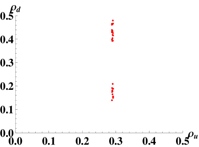
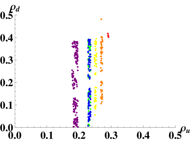
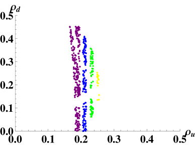
Figure 1: The dots represent the input values of ($\rho_{u},~{}\rho_{d}$) which yield the theoretical values of the mass ratios and the mixing angles within the range $0.2\leq{\rm th/ex}\leq 5.0$. We choose values of $\rho_{u}$ and $\rho_{d}$ from 0 to 0.5 randomly with $N=10^{4}$ trials for each combination $(\rho^{\prime}_{d},{\rm Im}\,\tau^{(1)})$ with $\rho^{\prime}_{d}=0.01~{},0.05,~{}0.1$ respectively from the top panel and ${\rm Im}\,\tau^{(1)}=1.5,~{}1.6,~{}1.7,~{}1.8,~{}1.9,~{}2.0$ distinguished by six colors, red, orange, yellow, green, blue and violet respectively. The suitable hierarchies are realized in wide regions.

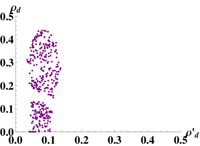
Figure 2: The dots represent the input values of ($\rho^{\prime}_{d},~{}\rho_{d}$) which yield the theoretical values of the mass ratios and the mixing angles within the range $0.2\leq{\rm th/ex}\leq 5.0$. We choose values of $\rho_{d}$ and $\rho^{\prime}_{d}$ from 0 to 0.5 randomly with $N=10^{4}$ trials for each combination of $(\rho_{u},{\rm Im}\,\tau^{(1)})=(0.3,1.45)$(the upper panel) and $(\rho_{u},{\rm Im}\,\tau^{(1)})=(0.2,1.95)$(the lower panel).

3.3 The 10D embedding and D-term contributions

We show an example of embedding our model into the 10D SYM theory with two independent $Z_{2}$ twists. We consider the magnetic fluxes on the second and the third tori as

$$F_{67}=2\pi\begin{pmatrix}0\times{\bm{1}}_{4}&0\\ 0&-{\bm{1}}_{4}\end{pmatrix},\hskip 20.0ptF_{89}=2\pi\begin{pmatrix}0\times{\bm{1}}_{4}&0\\ 0&{\bm{1}}_{4}\end{pmatrix}.$$ (42)

The SUSY condition (9) cannot be satisfied with the fluxes (10) and (42). We also consider the 10D orbifold $R^{3,1}\times T^{6}/(Z_{2}\times Z_{2}^{\prime})$. Under the $Z_{2}$ twist, the six toroidal coordinates transform as follows,

$$\left(y_{4},y_{5},y_{6},y_{7},y_{8},y_{9}\right)\rightarrow\left(-y_{4},-y_{5},-y_{6},-y_{7},y_{8},y_{9}\right),$$

and then, the transformations of the fields are already mentioned in Eq. (8) with the projection operator

$$P=\begin{pmatrix}-{\bm{1}}_{4}&0\\ 0&{\bm{1}}_{4}\end{pmatrix}.$$ (43)

The other, $Z_{2}^{\prime}$ is

$$\left(y_{4},y_{5},y_{6},y_{7},y_{8},y_{9}\right)\rightarrow\left(y_{4},y_{5},-y_{6},-y_{7},-y_{8},-y_{9}\right)$$ (44)

with the same projection operator as that of $Z_{2}$.

This background is consistent with the parity assignment on the first torus shown in Table 2 and does not change the flavor structure caused by the magnetic fluxes (10). We summarize all the contents induced by this background in Table 5.

	Fermions	Bosons	assignment
SM gauge fields	massless	massless	$A_{\mu},\lambda_{+++}$
$Q$	3 generations	heavy	$A_{6},A_{7},\lambda_{-+-}$
$u,d$	3 generations	heavy	$A_{8},A_{9},\lambda_{--+}$
$L$	3 generations	heavy	$A_{6},A_{7},\lambda_{-+-}$
$\nu,e$	3 generations	heavy	$A_{8},A_{9},\lambda_{--+}$
$H_{u},H_{d}$	massless	5 generations	$A_{4},A_{5},\lambda_{+--}$
Others	none	none	-

Table 5: All the contents of the model. The four types of $\lambda_{\pm\pm\pm}$ are the 4D Weyl spinors contained in the 10D Majorana-Weyl spinor, and each sign represents chiralities on the three tori. Others(i.e, $\lambda_{---}$) would never appear because of the 10D Majorana condition.

We obtain all the SM contents. Amazingly, there are no extra fields at all, such as exotic modes, vector-like matters and diagonal adjoint fields, so-called “open string moduli”. The existence of such extra massless fields is known as a notorious open problem in string phenomenology. Indeed, there necessarily exist some extra massless fields in our past works. In this model, the two orbifold twists and the magnetic fluxes free from the SUSY conditions eliminate them completely.

Finally, we estimate the spectrum of scalar particles caused by the non-SUSY background . Masses of scalar fields on a magnetized torus are given by [2]

$$M^{2}_{\rm scalar}=2\pi\frac{|M_{ab}|}{\mathcal{A}},$$

and also, those of vector fields are

$$M^{2}_{\pm}=2\pi\frac{|M_{ab}|}{\mathcal{A}}\pm 4\pi\frac{M_{ab}}{\mathcal{A}},$$

where $\pm$ represent mass eigenstates instead of the original 2D real vector (e.g., $(A_{4},A_{5})$). Each of $A_{m}$ behaves as a vector field on the corresponding torus as well as a scalar field on the other two tori. The masses in the 4D effective field theory are given by the sums of their eigenvalues on the three tori. Accordingly, we can estimate the heavy scalar spectrum, i.e. squarks and sleptons, as follows,

$$m^{2}_{\tilde{Q}} = 2\pi\left(\frac{5}{\mathcal{A}^{(1)}}+\frac{1}{\mathcal{A}^{(2)}}\pm 2\frac{1}{\mathcal{A}^{(2)}}+\frac{1}{\mathcal{A}^{(3)}}\right),$$

$$m^{2}_{\tilde{L}} = 2\pi\left(\frac{4}{\mathcal{A}^{(1)}}+\frac{1}{\mathcal{A}^{(2)}}\pm 2\frac{1}{\mathcal{A}^{(2)}}+\frac{1}{\mathcal{A}^{(3)}}\right),$$

$$m^{2}_{\tilde{u},\tilde{d}} = 2\pi\left(\frac{7}{\mathcal{A}^{(1)}}+\frac{1}{\mathcal{A}^{(2)}}+\frac{1}{\mathcal{A}^{(3)}}\pm 2\frac{1}{\mathcal{A}^{(3)}}\right),$$

$$m^{2}_{\tilde{e},\tilde{\nu}} = 2\pi\left(\frac{8}{\mathcal{A}^{(1)}}+\frac{1}{\mathcal{A}^{(2)}}+\frac{1}{\mathcal{A}^{(3)}}\pm 2\frac{1}{\mathcal{A}^{(3)}}\right),$$

and the contribution to the SM Higgs fields is

$$m^{2}_{H}=2\pi\left(\frac{12}{\mathcal{A}^{(1)}}\pm 2\frac{12}{\mathcal{A}^{(1)}}\right).$$

Therefore, the lightest scalar mode in the Higgs sector has a tachyonic mass of the order of the compactification scale. We find that, in any models with various 10D embeddings eliminating all the extra massless fields, tachyonic modes arise inevitably. We have to assume additional perturbative contributions to the soft scalar masses, and even some nonperturbative effects or higher dimensional operators to give them enough masses to cancel these tachyonic contributions. For example, other SUSY breaking contributions mediated by moduli, anomaly and gauge interactions are able to cancel the tachyonic $D$-term contributions. Another example is Wilson lines. It is known that Wilson lines without magnetic fluxes arise massive modes [18]. In the above example of 10D embedding, tachyonic Higgs fields have no fluxes on the two tori and a certain mass can be given by the Wilson lines. However, we have to remove the $Z_{2}^{\prime}$ projection (44) to introduce the Wilson lines. Even in such a case, the (MS)SM contents shown in Table 5 are unchanged, but there also remain some massless Wilson line moduli. We would study more about the stability of our 10D embeddings elsewhere.

4 Conclusions

We have realized a new-type of Yukawa structures in magnetized models with $Z_{2}$ orbifold twists. It is known that magnetic fluxes on a torus induce the chiral spectra and give them the degenerate (generation) structures. The magnitude of magnetic fluxes determine the number of generations, then, the orbifold projections give a variety of the model building with the three generations. We found such magnetized orbifold backgrounds do not preserve the 4D $\mathcal{N}=1$ SUSY , so in this paper, we have constructed a magnetized orbifold model with a non-SUSY background.

In Sec. 3, we have constructed the model, which can realize the experimental data of the quarks and the charged leptons simultaneously. For the purpose, we have chosen the different magnetic fluxes between the quark sector and the lepton sector under the condition that the down-sector quarks and the charged leptons couple with the same Higgs sector. Although the number of tunable parameters (VEVs) is extremely small in this model, we have been able to obtain the theoretical values of the masses and mixing angles, which is consistent with the experimental data, without fine-tunings. There is a reliable reason behind that, which has been revealed by our analysis of the Yukawa matrices.

The Yukawa matrix has the FN-like form with Gaussian hierarchies. The magnetic fluxes on the orbifold determine the “flavor quantum numbers” and give the new type of texture to the Yukawa matrices. We can get the theoretical values favored by the experiments in the wide parameter regions thanks to this new texture obtained from the wavefunction localization on the magnetized orbifold. We have also confirmed these analytic results numerically in the figures. We would expect such a FN-like Yukawa structure with Gaussian hierarchies inspires various phenomenological studies.

Finally, we have given a sample of embedding the above generation structure into the product of three tori in 10D spacetime, and studied the spectrum caused by the SUSY breaking magnetic fluxes. The magnetic fluxes and the orbifold twists can eliminate all the extra massless fields in this model, although some scalar fields will become tachyonic. Such a model free from extra massless fields has never realized on SUSY magnetized backgrounds.

Acknowledgement

H.A. and K.S. thank H. Kunoh for stimulating discussions in the early stage of this work. Y.T. would like to thank H. Ohki and Y. Yamada for useful discussions. H.A. was supported in part by the Grant-in-Aid for Scientific Research No. 25800158 from the Ministry of Education, Culture, Sports, Science and Technology (MEXT) in Japan. T.K. was supported in part by the Grant-in-Aid for Scientific Research No. 25400252 from the MEXT in Japan. K.S. was supported in part by a Grant-in-Aid for JSPS Fellows No. 25$\cdot$4968 and a Grant for Excellent Graduate Schools from the MEXT in Japan. Y.T. was supported in part by a Grant for Excellent Graduate Schools from the MEXT in Japan.

Appendix A Other flux configurations

We require that the magnetic fluxes in the quark sector are different from ones in the lepton sector, but the quarks and leptons couple with the same Higgs sector. The configuration in Table 2 satisfies this condition. Obviously, when we exchange the magnetic fluxes between the quark and lepton sectors (the left-handed and right-handed sectors), that also satisfies the condition. In addition, we have found the other configurations satisfying the condition.

The first one is that $M=-5$, $8$, and $-3$ for the left-handed quark, right-handed quark and Higgs sectors, and $M=-4$, $7$, and $-3$ for the left-handed lepton, right-handed lepton and Higgs sectors including the exchange of magnetic fluxes between the quark and lepton sectors (the left-handed and right-handed sectors). These lead to one-pair Higgs doublets just like the MSSM, but the Yukawa matrices do not have the Gaussian Froggatt-Nielsen texture. (We can easily see that they are phenomenologically disfavored.)

The second has a five-block structure breaking the $SU(2)_{R}$ symmetry. That is shown in Table 6 or with the quark/lepton exchange.

$Q$	$L$	$U$	$D$	$N$	$E$	$H_{u}$	$H_{d}$
$-4$ (even)	$-5$ (even)	$-5$ (even)	$-8$ (odd)	$-4$ (even)	$-7$ (odd)	$9$ (even)	$12$ (odd)

Table 6: Magnetic fluxes felt by each sector with $SU(2)_{R}$ breaking.

This configuration breaks the $SU(2)_{R}$ symmetry. However, the values of up- and down-type Higgs VEVs could not be predicted practically, because they are depending on other parts of this model and the relevant Higgs phenomenologies, which are not the purpose and we will not mention it in this paper. Since the neutrino Yukawa matrix $y_{\nu}$ is the transpose of up-type quark Yukawa matrix $y_{u}$ and the (Dirac) mass hierarchies among the three generations are the same in the two sectors, we cannot exchange the magnetic fluxes between up and down sectors.

In the model shown in Table 2, the three generations are obtained by the magnetic fluxes, ($M_{ab}=-5$, $M_{bc}=-7$, $M_{ca}=12$) or ($M_{ab}=-4$, $M_{bc}=-8$, $M_{ca}=12$). $Y_{3+4}$, which is defined above Eq. (15), with the two types of fluxes have the Gaussian Froggatt-Nielsen texture. The matrix $Y_{3+4}$ can be approximated by

$$y_{ij}\sim e^{-\pi({\rm Im}\tau)(a_{i}+b_{j})^{2}/M_{ab}M_{bc}M_{ca}}$$ (45)

with ($a_{i}=20,~{}10,~{}0$) and ($b_{i}=10,~{}5,~{}0$) for ($M_{ab}=-5$, $M_{bc}=-7$, $M_{ca}=12$), and with ($a_{i}=20,~{}5,~{}0$) and ($b_{i}=15,~{}5,~{}0$) for ($M_{ab}=-4$, $M_{bc}-8$, $M_{ca}=12$). The five-block model shown in Table 6 contains a new type of that, that is, ($M_{ab}=-4$, $M_{bc}=-5$, $M_{ca}=9$). These fluxes also induce the five generations of Higgs multiplets, and then, $Y_{3+4}$ has the Gaussian Froggatt-Nielsen texture and can be written by Eq. (45) with ($a_{i}=10,~{}5,~{}0$) and ($b_{i}=10,~{}5,~{}0$).

References

- [1] C. Bachas, hep-th/9503030; C. Angelantonj, I. Antoniadis, E. Dudas and A. Sagnotti, Phys. Lett. B 489 (2000) 223 [hep-th/0007090].
- [2] D. Cremades, L. E. Ibanez and F. Marchesano, JHEP 0405 (2004) 079 [hep-th/0404229].
- [3] H. Abe, T. Kobayashi, H. Ohki, A. Oikawa and K. Sumita, Nucl. Phys. B 870 (2013) 30 [arXiv:1211.4317 [hep-ph]].
- [4] H. Abe, T. Kobayashi, H. Ohki, K. Sumita and Y. Tatsuta, arXiv:1307.1831 [hep-th].
- [5] H. Abe, T. Kobayashi and H. Ohki, JHEP 0809 (2008) 043 [arXiv:0806.4748 [hep-th]].
- [6] H. Abe, K. -S. Choi, T. Kobayashi and H. Ohki, Nucl. Phys. B 814 (2009) 265 [arXiv:0812.3534 [hep-th]].
- [7] H. Abe, K. -S. Choi, T. Kobayashi and H. Ohki, Phys. Rev. D 80 (2009) 126006 [arXiv:0907.5274 [hep-th]].
- [8] T. -H. Abe, Y. Fujimoto, T. Kobayashi, T. Miura, K. Nishiwaki and M. Sakamoto, JHEP 1401, 065 (2014) [arXiv:1309.4925 [hep-th]].
- [9] M. Kobayashi and T. Maskawa, Prog. Theor. Phys. 49 (1973) 652.
- [10] H. Abe, T. Kobayashi, H. Ohki and K. Sumita, Nucl. Phys. B 863 (2012) 1 [arXiv:1204.5327 [hep-th]].
- [11] H. Kunoh, Master thesis submitted to Waseda University (2012).
- [12] J. Beringer et al. [Particle Data Group Collaboration], Phys. Rev. D 86 (2012) 010001.
- [13] R. Blumenhagen, M. Cvetic and T. Weigand, Nucl. Phys. B 771, 113 (2007) [hep-th/0609191]; L. E. Ibanez and A. M. Uranga, JHEP 0703, 052 (2007) [hep-th/0609213]; L. E. Ibanez, A. N. Schellekens and A. M. Uranga, JHEP 0706, 011 (2007) [arXiv:0704.1079 [hep-th]]; S. Antusch, L. E. Ibanez and T. Macri, JHEP 0709, 087 (2007) [arXiv:0706.2132 [hep-ph]]; Y. Hamada, T. Kobayashi and S. Uemura, arXiv:1402.2052 [hep-th].
- [14] C. D. Froggatt and H. B. Nielsen, Nucl. Phys. B 147 (1979) 277.
- [15] L. E. Ibanez and G. G. Ross, Phys. Lett. B 332, 100 (1994) [hep-ph/9403338]; P. Binetruy and P. Ramond, Phys. Lett. B 350, 49 (1995) [hep-ph/9412385]; E. Dudas, S. Pokorski and C. A. Savoy, Phys. Lett. B 356, 45 (1995) [hep-ph/9504292].
- [16] T. Gherghetta and A. Pomarol, Nucl. Phys. B 586, 141 (2000) [hep-ph/0003129]; S. J. Huber and Q. Shafi, Phys. Lett. B 498, 256 (2001) [hep-ph/0010195]; H. Abe, T. Kobayashi, N. Maru and K. Yoshioka, Phys. Rev. D 67, 045019 (2003) [hep-ph/0205344]; K. -w. Choi, D. Y. Kim, I. -W. Kim and T. Kobayashi, Eur. Phys. J. C 35, 267 (2004) [hep-ph/0305024].
- [17] A. E. Nelson and M. J. Strassler, JHEP 0009, 030 (2000) [hep-ph/0006251]; JHEP 0207, 021 (2002) [hep-ph/0104051]; T. Kobayashi and H. Terao, Phys. Rev. D 64, 075003 (2001) [hep-ph/0103028].
- [18] Y. Hamada and T. Kobayashi, Prog. Theor. Phys. 128 (2012) , 903 [arXiv:1207.6867 [hep-th]].