On the construction of $m$-step methods for FDEs

Abstract

In this paper we consider the numerical solution of Fractional Differential Equations by means of $m$-step recursions. The construction of such formulas can be obtained in many ways. Here we study a technique based on the rational approximation of the generating functions of Fractional Backward Differentiation Formulas (FBDFs). Accurate approximations allow to define methods which simulate the theoretical properties of the underlying FBDF with important computational advantages. Numerical experiments are presented.

MSC: 65L06, 65F60, 65D32, 26A33, 34A08.

1 Introduction

This paper deals with the solution of Fractional Differential Equations (FDEs) of the type

$${}_{t_{0}}D_{t}^{\alpha}y(t)=g(t,y(t)),\quad t_{0}<t\leq T,\quad 0<\alpha<1,$$ (1)

where ${}_{t_{0}}D_{t}^{\alpha}$ denotes the Caputo’s fractional derivative operator (see e.g. [16] for an overview) defined as

$${}_{t_{0}}D_{t}^{\alpha}y(t)=\frac{1}{\Gamma(1-\alpha)}\int_{t_{0}}^{t}\frac{y^{\prime}(u)}{(t-u)^{\alpha}}du,$$ (2)

in which $\Gamma$ denotes the Gamma function. As well known, the use of the Caputo’s definition for the fractional derivative allows to treat the initial conditions at $t_{0}$ for FDEs in the same manner as for integer order differential equations. Setting $y(t_{0})=y_{0}$ the solution of (1) exists and is unique under the hypothesis that $g$ is continuous and fulfils a Lipschitz condition with respect to the second variable (see e.g. [3] for a proof).

As for the integer order case $\alpha=1$, a classical approach for solving (1) is based on the discretization of the fractional derivative (2), which generalizes the well known Grunwald-Letnikov discretization (see [16, §2.2]), leading to the so-called Fractional Backward Differentiation Formulas (FBDFs) introduced in [12]. Taking a uniform mesh $t_{0},t_{1},\dots,t_{N}=T$ of the time domain with stepsize $h=(T-t_{0})/N,$ FBDFs are based on the full-term recursion

$$\sum\nolimits_{j=0}^{n}\omega_{n-j}^{(p)}y_{j}=h^{\alpha}g(t_{n},y_{n}),\quad p\leq n\leq N,$$ (3)

where $y_{j}\approx y(t_{j})$ and $\omega_{n-j}^{(p)}$ are the Taylor coefficients of the generating function

$$\omega_{p}^{(\alpha)}(\zeta) = \left(a_{0}+a_{1}\zeta+...+a_{p}\zeta^{p}\right)^{\alpha}$$ (4)

$$= \sum\nolimits_{i=0}^{\infty}\omega_{i}^{(p)}\zeta^{i},\quad\text{for}\quad 1\leq p\leq 6,$$ (5)

being $\left\{a_{0},a_{1},\dots,a_{p}\right\}$ the coefficients of the underlying BDF. In [12] it is also shown that the order $p$ of the BDF is preserved.

We remember that for this kind of equations, there is generally an intrinsic lack of regularity of the solution in a neighborhood of the starting point, that is, depending on the function $g$, one may have $y(t)\sim(t-t_{0})^{\alpha}$ as $t\rightarrow t_{0}$. For this reason, in order to preserve the theoretical order $p$ of the numerical method, formula (3) is generally corrected as

$$\sum\nolimits_{j=0}^{M}w_{n,j}y_{j}+\sum\nolimits_{j=0}^{n}\omega_{n-j}^{(p)}y_{j}=h^{\alpha}g(t_{n},y_{n}),$$ (6)

where the sum $\sum\nolimits_{j=0}^{M}w_{n,j}y_{j}$ is the so-called starting term, in which $M$ and the weights $w_{n,j}$ depend on $\alpha$ and $p$ (see [2, Chapter 6] for a discussion).

Denoting by $\Pi_{m}$ the set of polynomials of degree not exceeding $m$, our basic idea is to design methods based on rational approximations of (4), i.e.,

$$R_{m}(\zeta)\approx\omega_{p}^{(\alpha)}(\zeta),\quad R_{m}(\zeta)=\frac{p_{m}(\zeta)}{q_{m}(\zeta)},\quad p_{m},q_{m}\in\Pi_{m}.$$ (7)

Writing $p_{m}(\zeta)=\sum\nolimits_{j=0}^{m}\alpha_{j}\zeta^{j}$ and $q_{m}(\zeta)=\sum\nolimits_{j=0}^{m}\beta_{j}\zeta^{j}$, the above approximation naturally leads to implicit $m$-step recursions of the type

$$\sum\nolimits_{j=n-m}^{n}\alpha_{n-j}y_{j}=h^{\alpha}\sum\nolimits_{j=n-m}^{n}\beta_{n-j}g(t_{j},y_{j}),\quad n\geq m.$$ (8)

While the order of the FBDF is lost, we shall see that if the approximation (7) is rather accurate, then (8) is able to produce reliable approximations to the solution. Starting from the initial data $y(t_{0})=y_{0}$, the first $m-1$ approximations $y_{1},\ldots,y_{m-1}$ can be generated by the underlying FBDFs or even considering lower degree rational approximations.

A formula of type (8) generalizes in some sense the methods based on the Short Memory Principle in which the truncated Taylor expansion of (4) is considered (see [16, §8.3] for some examples). Computationally, the advantages are noticeable, especially in terms of memory saving whenever (1) arises from the semi-discretization of fractional partial differential equations. We remark moreover that since the initial approximations are used only at the beginning of the process, there is no need to use a starting term to preserve the theoretical order as for standard full-recursion multistep formulas. Moreover, as remarked in [4], in particular when $\alpha\neq 1/2$, the use of a starting formula as in (6), that theoretically should ensure the order of the FBDF, in practice may introduce substantial errors, causing unreliable numerical solutions. For high-order formulas, this is due to the severe ill-conditioning of the Vandermonde type systems one has to solve at each integration step to generate the weights $w_{n,j}$ of the starting term. We also remark that in a typical application $\alpha$, $y_{0}$ and possibly also the function $g$ may be only known up to a certain accuracy (see [3] for a discussion), so that one may only be interested in having a rather good approximation of the true solution.

For the construction of formulas of type (8), in this paper we present a technique based on the rational approximation of the fractional derivative operator (cf. [14]). After considering a BDF discretization of order $p$ of the first derivative operator, which can be represented by a $N\times N$ triangular banded Toeplitz matrix $A_{p}$, we approximate Caputo’s fractional differential operator ${}_{t_{0}}D_{t}^{\alpha}$ by calculating $A_{p}^{\alpha}$. This computation is performed by means of the contour integral approximation, which leads to a rational approximation of $A_{p}^{\alpha}$ whose coefficients can be used to define (8). This technique is based on the fact that the first column of $A_{p}^{\alpha}$ contains the first $N$ coefficients of the Taylor expansion of $\omega_{p}^{(\alpha)}(\zeta)$, so exploiting the equivalence between the approximation of $A_{p}^{\alpha}$ and $\omega_{p}^{(\alpha)}(\zeta)$.

The outline of the paper is the following. As in [5], the contour integral is evaluated by means of the Gauss-Jacobi rule in Section 2. An error analysis of this approach is outlined in Section 3, together with some numerical experiments that confirm its effectiveness. In Section 4 we investigate the reliability of this approach for the solution of fractional differential equations. In particular, we present some results concerning the consistency and the linear stability. Finally, in Section 5 we consider the results of the method when applied to the discretization of two well-known models of fractional diffusion.

2 The approximation of the fractional derivative operator

Denoting by $a_{0},a_{1},\dots,a_{p}$ the $p+1$ coefficients of a Backward Differentiation Formula (BDF) of order $p$, with $1\leq p\leq 6$, which discretizes the derivative operator (see [8, Chapter III.1] for a background), we consider lower triangular banded Toeplitz matrices of the type

$$A_{p}=\left(\begin{array}[]{ccccc}a_{0}&0&&&0\\ \vdots&a_{0}&0&&\\ a_{p}&\vdots&\ddots&0&\\ 0&\ddots&&\ddots&0\\ &0&a_{p}&\cdots&a_{0}\end{array}\right)\in\mathbb{R}^{(N+1)\times(N+1)}.$$ (9)

In this setting, $A_{p}^{\alpha}e_{1}$, $e_{1}=(1,0,\dots,0)^{T}$, contains the whole set of coefficients of the corresponding FBDF for approximating the solution of (1) in $t_{0},t_{1},\dots,t_{N}$, that is

$$e_{j+1}^{T}A_{p}^{\alpha}e_{1}=\omega_{j}^{(p)},\quad 0\leq j\leq N,$$ (10)

(cf. (5)). The constraint $p\leq 6$ is due to the fact that BDFs are not zero-stable for $p>6.$

From the theory of matrix functions (see [10] for a survey), we know that the fractional power of matrix can be written as a contour integral

$$A^{\alpha}=\frac{A}{2\pi i}\int_{\Gamma}z^{\alpha-1}(zI-A)^{-1}dz,$$

where $\Gamma$ is a suitable closed contour enclosing the spectrum of $A$, $\sigma(A)$, in its interior. The following known result (see, e.g., [1]) expresses $A^{\alpha}$ in terms of a real integral.

Proposition 1

Let $A\in\mathbb{R}^{N\times N}$ be such that $\sigma(A)\subset\mathbb{C}\backslash\left(-\infty,0\right]$. For $0<\alpha<1$ the following representation holds

$$A^{\alpha}=\frac{A\sin(\alpha\pi)}{\alpha\pi}\int_{0}^{\infty}(\rho^{1/\alpha}I+A)^{-1}d\rho.$$ (11)

Of course the above result holds also in our case since $\sigma(A_{p})=\{a_{0}\}$ and $a_{0}>0$ for each $1\leq p\leq 6.$ At this point, for each suitable change of variable for $\rho$, a $k$-point quadrature rule for the computation of the integral in (11) yields a rational approximation of the type

$$A_{p}^{\alpha}\approx A_{p}\widetilde{R}_{k}(A_{p}):=A_{p}\sum\nolimits_{j=1}^{k}\gamma_{j}(\eta_{j}I+A_{p})^{-1},$$ (12)

where the coefficients $\gamma_{j}$ and $\eta_{j}$ depend on the substitution and the quadrature formula. This technique has been used in [14], where the author applies the Gauss-Legendre rule to (11) after the substitution

$$\rho=a_{0}^{\alpha}\left(\cos\theta\right)^{-\alpha/(1-\alpha)}\sin\theta,$$

which generalizes the one presented in [9] for the case $\alpha=1/2.$

In order to remove the dependence of $\alpha$ inside the integral we consider the change of variable

$$\rho^{1/\alpha}=\tau\frac{1-t}{1+t},\qquad\tau>0,$$ (13)

yielding

$$\frac{1}{\alpha}\int_{0}^{\infty}(\rho^{1/\alpha}I+A_{p})^{-1}d\rho$$

$$= 2\int_{-1}^{1}\left(\tau\frac{1-t}{1+t}\right)^{\alpha-1}\left(\tau\frac{1-t}{1+t}I+A_{p}\right)^{-1}\frac{\tau}{\left(1+t\right)^{2}}dt$$

$$= 2\tau^{\alpha}\int_{-1}^{1}\left(1-t\right)^{\alpha-1}\left(1+t\right)^{-\alpha}\left(\tau\left(1-t\right)I+\left(1+t\right)A_{p}\right)^{-1}dt,$$

and hence

$$A_{p}^{\alpha}=\frac{2\sin(\alpha\pi)\tau^{\alpha}}{\pi}A_{p}\int_{-1}^{1}\left(1-t\right)^{\alpha-1}\left(1+t\right)^{-\alpha}\left(\tau\left(1-t\right)I+\left(1+t\right)A_{p}\right)^{-1}dt.$$ (14)

The above formula naturally leads to the use of a $k$-point Gauss-Jacobi rule for the approximation of $A_{p}^{\alpha}e_{1}$ and hence to a rational approximation (12).

The following result can be proved by direct computation.

Proposition 2

Let $A_{p}\in\mathbb{R}^{N\times N}$ be a matrix of type (9), and let $\overline{A}_{p}=\frac{1}{a_{0}}A_{p}$. Then the components of $(\xi I+\overline{A}_{p})^{-1}e_{1}$, $\xi\neq-1$, are given by

$$\upsilon_{1}^{(p)}(\xi) = \frac{1}{\xi+1},$$

$$\upsilon_{j}^{(p)}(\xi) = \frac{c_{2,j}^{(p)}}{\left(\xi+1\right)^{2}}+\ldots+\frac{c_{j,j}^{(p)}}{\left(\xi+1\right)^{j}},\quad 2\leq j\leq N,$$

where the coefficients $c_{i,j}^{(p)}$ depend on the order $p$. For $p=1$ we simply have $\left\{a_{0},a_{1}\right\}=\left\{1,-1\right\}$, and hence

$$\upsilon_{j}^{(1)}(\xi)=\frac{1}{\left(\xi+1\right)^{j}},\quad 1\leq j\leq N.$$

The above proposition shows that the components of

$$\left(\tau\left(1-t\right)I+\left(1+t\right)A_{p}\right)^{-1}e_{1}$$

are analytic functions in a suitable open set containing $[-1,1]$ in its interior, since they are sum of functions of the type

$$\frac{\left(1+t\right)^{l-1}}{\left(\tau\left(1-t\right)+a_{0}\left(1+t\right)\right)^{l}},\quad l\geq 1,$$ (15)

whose pole lies outside $[-1,1]$ for $\tau>0$ (recall that $a_{0}>0$ for $1\leq p\leq 6$). In this sense, the lack of regularity of the integrand in (14) due to the presence of $\alpha,$ is completely absorbed by the Jacobi weight function so that the Gauss-Jacobi rule yields a very efficient tool for the computation of $A_{p}^{\alpha}$.

Increasing $k$ the approximation (12) can be used to approximate the whole set of coefficients of the FBDFs. We remark that the computation of the vectors $(\eta_{j}I+A_{p})^{-1}e_{1}$ does not constitute a problem because of the structure of $A_{p}$ (see (9)). We also point out that since our aim is to construct reliable formulas of type (8) we actually do not need to evaluate (12). Indeed we just need to know the scalars $\gamma_{j}$ and $\eta_{j}$, and then, using an algorithm to transform partial fractions to polynomial quotient, we obtain the approximation

$$z^{\alpha}\approx z\widetilde{R}_{k}(z)=z\frac{\widetilde{p}_{k-1}(z)}{\widetilde{q}_{k}(z)},\quad z=a_{0}+a_{1}\zeta+\ldots+a_{p}\zeta^{p},$$ (16)

where $\widetilde{p}_{k-1}\in\Pi_{k-1}$ and $\widetilde{q}_{k}\in\Pi_{k}.$ This finally leads to the approximation (7) with

$$p_{m}(\zeta) = (a_{0}+a_{1}\zeta+\ldots+a_{p}\zeta^{p})\,\widetilde{p}_{k-1}(a_{0}+a_{1}\zeta+\ldots+a_{p}\zeta^{p}),$$ (17)

$$q_{m}(\zeta) = \widetilde{q}_{k}(a_{0}+a_{1}\zeta+\ldots+a_{p}\zeta^{p}),$$ (18)

in which $m=kp$. We remark that whenever the procedure for the definition of the coefficients $\gamma_{j}$ and $\eta_{j}$ has been set for a given $\alpha,$ one can compute the corresponding coefficients in the $m$-step formula (8) once and for all.

3 Theoretical error analysis

Denoting by $J_{k}(A_{p})$ the result of the Gauss-Jacobi rule for the approximation of

$$J(A_{p})=\int_{-1}^{1}\left(1-t\right)^{\alpha-1}\left(1+t\right)^{-\alpha}\left(\tau\left(1-t\right)I+\left(1+t\right)A_{p}\right)^{-1}dt,$$

by (14) the corresponding approximation to $A_{p}^{\alpha}$ is given by

$$A_{p}^{\alpha}\approx A_{p}\widetilde{R}_{k}(A_{p}),\qquad\widetilde{R}_{k}(A_{p})=\frac{2\sin(\alpha\pi)\tau^{\alpha}}{\pi}J_{k}(A_{p}).$$ (19)

In this section we analyze the error term componentwise, that is, (see (10),

$$E_{j} := \omega_{j}^{(p)}-e_{j+1}^{T}A_{p}\widetilde{R}_{k}(A_{p})e_{1}=e_{j+1}^{T}A_{p}\left(A_{p}^{\alpha-1}-\widetilde{R}_{k}(A_{p})\right)e_{1}$$

$$= \frac{2\sin(\alpha\pi)\tau^{\alpha}}{\pi}e_{j+1}^{T}A_{p}\left(J(A_{p})-J_{k}(A_{p})\right)e_{1},\quad 0\leq j\leq N,$$

which is the error in the computation of the $j$-th coefficient of the Taylor expansion of $\omega_{p}^{(\alpha)}(\zeta)$. Numerically one observes that the quality of the approximation tends to deteriorate when the dimension of the problem $N$ grows. In this sense we are particularly interested in observing the dependence of the error term on $j$ and $k$ for $j\gg k$ and to find a strategy to define the parameter $\tau$ of the substitution (13) in this situation. As we shall see in the remainder of the paper, this parameter plays a crucial role for the quality of the approximation.

We restrict our analysis to the case of $p=1$ for which $a_{0}=-a_{1}=1.$ In this situation, defining the vector

$$r:=\left(J(A_{1})-J_{k}(A_{1})\right)e_{1},$$ (21)

we have that

$$E_{j}=\frac{2\sin(\alpha\pi)\tau^{\alpha}}{\pi}e_{j+1}^{T}A_{1}r,$$

and therefore

$$\left|E_{j}\right|\leq\frac{2\sin(\alpha\pi)\tau^{\alpha}}{\pi}\left(\left|r_{j}\right|+\left|r_{j-1}\right|\right).$$ (22)

The analysis thus reduces to the study of the components of the vector (21). By Proposition 2, see also (15), the $j$-th component of the vector

$$\left(\tau\left(1-t\right)I+\left(1+t\right)A_{1}\right)^{-1}e_{1}$$

is given by

$$f_{j}(t)=\frac{\left(1+t\right)^{j-1}}{\left(\tau(1-t)+1+t\right)^{j}},$$ (23)

so that $r_{j}$ is the error term of the $k$-point Gauss-Jacobi formula applied to the computation of

$$\int_{-1}^{1}\left(1-t\right)^{\alpha-1}\left(1+t\right)^{-\alpha}f_{j}(t)dt.$$ (24)

We start with the following known result, [11].

Theorem 1

The error term of the $k$-point Gauss-Jacobi formula applied to the computation of

$$\int\nolimits_{-1}^{1}(1-t)^{\alpha_{1}}(1+t)^{\alpha_{2}}g(t)dt,\quad\alpha_{1},\alpha_{2}>-1,\quad g\in C^{2k}([-1,1]),$$

is given by

$$C_{k,\alpha_{1},\alpha_{2}}g^{(2k)}(\xi),\quad-1<\xi<1,$$

where

$$C_{k,\alpha_{1},\alpha_{2}}:=\frac{\Gamma(k+\alpha_{1}+1)\Gamma(k+\alpha_{2}+1)\Gamma(k+\alpha_{1}+\alpha_{2}+1)k!}{(2k+\alpha_{1}+\alpha_{2}+1)\left[\Gamma(2k+\alpha_{1}+\alpha_{2}+1)\right]^{2}(2k)!}2^{2k+\alpha_{1}+\alpha_{2}+1}.$$ (25)

Lemma 1

Let $0<\alpha<1$ and $C_{k,\alpha}:=C_{k,\alpha-1,-\alpha}$. Then

$$C_{k,\alpha}\sim\frac{\pi 2^{1-2k}}{(2k)!}.$$

Proof. By (25) we easily obtain

$$C_{k,\alpha}=\frac{\Gamma(k+\alpha)\Gamma(k-\alpha+1)\left[\Gamma(k)\right]^{2}}{\left[\Gamma(2k)\right]^{2}(2k)!}2^{2k-1}.$$

Using the Legendre formula

$$\Gamma\left(k+\frac{1}{2}\right)\Gamma(k)=\sqrt{\pi}\Gamma(2k)2^{1-2k},$$

we have that

$$C_{k,1/2}=\frac{\pi 2^{1-2k}}{(2k)!}.$$

Moreover, since for $a,b\in(0,1)$

$$k^{b-a}\frac{\Gamma(k+a)}{\Gamma(k+b)}=1+O\left(\frac{1}{k}\right),$$

we have that $\Gamma(k+\alpha)\Gamma(k-\alpha+1)=\left[\Gamma(k+\frac{1}{2})\right]^{2}(1+O(k^{-1}))$ and, consequently, $C_{k,\alpha}\rightarrow C_{k,1/2}$ as $k\rightarrow\infty$.   

Remark 1

If we set $\tau=1$ in (13) we obtain $r_{j}=0$ for each $j=1,2,\ldots,2k$ since $f_{j}\in\Pi_{j-1},$ see (23). From (16), with $p=1,$ and (19) one therefore gets

$$(1-\zeta)^{\alpha-1}-\widetilde{R}_{k}(1-\zeta)=(1-\zeta)^{\alpha-1}-\frac{\widetilde{p}_{k-1}(1-\zeta)}{\widetilde{q}_{k}(1-\zeta)}=O(\zeta^{2k}),$$

so that $\widetilde{R}_{k}(1-\zeta)$ is the $(k-1,k)$ Padé approximant of $(1-\zeta)^{\alpha-1}$ with expansion point $\zeta=0.$ More generally, if $\tau\in(0,1]$ then the resulting rational approximation coincides with the same Padé approximant with expansion point $\zeta=1-\tau\$(cf. [5, Lemma 4.4]).

Numerically, it is quite clear that the best results are obtained for $\tau$ strictly less than 1, so that in what follows we always assume to work with $\tau\in(0,1)$. Indeed, in this situation we are able to approximate the Taylor coefficients with a more uniform distribution of the error with respect to $j.$ By Theorem 1, we need to bound $\left|f_{j}^{(2k)}(t)\right|$ in the interval $[-1,1]$ in order to bound the error term $E_{j}.$ We start with the following result.

Proposition 3

Let $0<\tau<1\$and

$$a:=\frac{1+\tau}{1-\tau}.$$ (26)

For each $j$ and $k$

$$\max_{[-1,1]}\left|f_{j}^{(2k)}(t)\right|\leq\left(2k\right)!\frac{\sqrt{a}}{\left(\sqrt{a}-1\right)^{2k+2}}\left(\frac{a+1}{2\sqrt{a}}\right)^{j}.$$

Proof. The function $f_{j}$ can be written as

$$f_{j}(t)=\frac{\left(1+t\right)^{j-1}}{\left(a+t\right)^{j}}\left(\frac{a+1}{2}\right)^{j},\quad a>1.$$

Using the Cauchy integral formula we have

$$f_{j}^{(2k)}(t)=\frac{\left(2k\right)!}{2\pi i}\int_{\Gamma}\frac{f_{j}(w)}{\left(w-t\right)^{2k+1}}dw,$$ (27)

where $\Gamma$ is a contour surrounding $t$ but not the pole $-a<-1$. We take $\Gamma$ as the circle centered at the origin and radius $\rho$ such that $1<\rho<a$, that is, we use the substitution $w=\rho e^{i\theta}$. We obtain

$$\max_{[-1,1]}\left|f_{j}^{(2k)}(t)\right|\leq\left(2k\right)!\frac{\rho}{\left(\rho-1\right)^{2k+1}}\max_{[0,2\pi]}\left|f_{j}(\rho e^{i\theta})\right|.$$ (28)

Taking $\rho=\sqrt{a}$ we have

$$\left|f_{j}(\rho e^{i\theta})\right| = \left|\frac{1}{1+\rho e^{i\theta}}\right|\left|\frac{1+\rho e^{i\theta}}{a+\rho e^{i\theta}}\right|^{j}\left(\frac{a+1}{2}\right)^{j}$$

$$= \left|\frac{1}{1+\sqrt{a}e^{i\theta}}\right|\left|\frac{1+\sqrt{a}e^{i\theta}}{a+\sqrt{a}e^{i\theta}}\right|^{j}\left(\frac{a+1}{2}\right)^{j}$$

$$= \left|\frac{1}{1+\sqrt{a}e^{i\theta}}\right|\left(\frac{a+1}{2\sqrt{a}}\right)^{j}$$

$$\leq \frac{1}{\left(\sqrt{a}-1\right)}\left(\frac{a+1}{2\sqrt{a}}\right)^{j}.$$

By (28) we immediately achieve the result.   

The above result is rather accurate only for small values of $j$. Since $f_{j}(t)$ is growing in the interval $[-1,1]$, below we consider contours $\Gamma$ in (27) which are dependent on $t$, in order to balance this effect.

Proposition 4

Let $0<\tau<1\$ and $a$ as in (26). For $j\geq 2k+2$

$$\left|f_{j}^{(2k)}(t)\right|\leq\left(2k\right)!\frac{\sqrt{a+1}+\sqrt{2}}{a-1}\frac{\left(1+t\right)^{\frac{j-1}{2}-k}}{(a+t)^{\frac{j}{2}+k}}\left(\frac{a+1}{2}\right)^{j},\quad t\in[-1,1].$$ (29)

Moreover

$$\max_{[-1,1]}\left|f_{j}^{(2k)}(t)\right|\leq\left(2k\right)!\left(\sqrt{a+1}+\sqrt{2}\right)\frac{\left(\frac{j-2k-1}{4k+1}\right)^{\frac{j-1}{2}-k}}{\left(\frac{j+2k}{4k+1}\right)^{\frac{j}{2}+k}}\left(\frac{a+1}{2}\right)^{j}\left(a-1\right)^{-2k-\frac{3}{2}}$$ (30)

for $j$ such that

$$a\leq\frac{j+6k+1}{j-2k-1},$$ (31)

and

$$\max_{[-1,1]}\left|f_{j}^{(2k)}(t)\right|\leq\left(2k\right)!\frac{\sqrt{a+1}+\sqrt{2}}{a-1}\frac{\left(a+1\right)^{\frac{j}{2}-k}}{2^{\frac{j+1}{2}+k}}$$ (32)

otherwise.

Proof. In (27) we take $\Gamma$ as the circle centered at $t$ and of radius $\rho$ such that $1+t<\rho<t+a$, that is, we use the substitution $w=t+\rho e^{i\theta}$. We obtain

$$\left|f_{j}^{(2k)}(t)\right|\leq\left(2k\right)!\frac{1}{\rho^{2k}}\max_{[0,2\pi]}\left|f_{j}(t+\rho e^{i\theta})\right|.$$ (33)

For $t>-1$ we define $\rho=\sqrt{(t+a)(1+t)}$, so that

$$\left|f_{j}(t+\rho e^{i\theta})\right| = \left|\frac{1}{1+t+\rho e^{i\theta}}\right|\left|\frac{1+t+\rho e^{i\theta}}{a+t+\rho e^{i\theta}}\right|^{j}\left(\frac{a+1}{2}\right)^{j}$$

$$= \left|\frac{1}{1+t+\sqrt{(t+a)(1+t)}e^{i\theta}}\right|\times$$

$$\left|\frac{1+t+\sqrt{(t+a)(1+t)}e^{i\theta}}{a+t+\sqrt{(t+a)(1+t)}e^{i\theta}}\right|^{j}\left(\frac{a+1}{2}\right)^{j}$$

$$= \left|\frac{1}{1+t+\sqrt{(t+a)(1+t)}e^{i\theta}}\right|\left(\frac{1+t}{a+t}\right)^{\frac{j}{2}}\left(\frac{a+1}{2}\right)^{j},$$

and hence

$$\max_{[0,2\pi]}\left|f_{j}(t+\rho e^{i\theta})\right| = \frac{1}{\sqrt{(t+a)(1+t)}-(1+t)}\left(\frac{1+t}{a+t}\right)^{\frac{j}{2}}\left(\frac{a+1}{2}\right)^{j}$$

$$= \frac{\sqrt{(t+a)}+\sqrt{(1+t)}}{\sqrt{(1+t)}(a-1)}\left(\frac{1+t}{a+t}\right)^{\frac{j}{2}}\left(\frac{a+1}{2}\right)^{j}.$$

By (33) we obtain the bound (29) for each $j$ and $k$, for $t>-1$. By continuity, (29) holds for $t\in[-1,1]$ if $j\geq 2k+2$.

Now, we observe that the maximum with respect to $t$ of the function

$$\frac{\left(1+t\right)^{\frac{j-1}{2}-k}}{(a+t)^{\frac{j}{2}+k}}$$

is attained at

$$t^{\ast}=\frac{a(j-2k-1)-(j+2k)}{4k+1}\geq-1.$$

Moreover $t^{\ast}\leq 1$ for $a$ verifying (31). Substituting $t^{\ast}$ in (29) leads to (30). If $t^{\ast}>1$ then the maximum of (29) is reached at $t=1$ and hence we obtain (32).   

In order to derive (30) and (32) we have assumed $\tau$ to be a priori fixed. Now, using these bounds, we look for the value of $\tau$ which minimize $\left\|f_{j}^{(2k)}\right\|$ for a given $j$. For $j\geq 2k+3$, the minimization of the term

$$\left(a+1\right)^{j}\left(a-1\right)^{-2k-\frac{3}{2}}$$

in (30) leads to

$$a^{(1)}=\frac{2j+4k+3}{2j-4k-3},$$

which satisfies (31). Consequently, by (26) we obtain

$$\tau^{(1)}=\frac{4k+3}{2j}.$$ (34)

On the other side, for the same $j\geq 2k+3,$ the minimization of the term

$$\frac{\sqrt{a+1}+\sqrt{2}}{a-1}\left(a+1\right)^{\frac{j}{2}-k}$$

in (32) leads to a value

$$a^{\ast}\leq\frac{j-2k+2}{j-2k-2},$$

which also satisfies (31) and hence does not fulfill the requirement of (32). For $a>a^{\ast}$ the bound (32) is growing with $a$ and consequently its minimum is attained just for

$$a^{(2)}=\frac{j+6k+1}{j-2k-1}.$$

Using this value in (32) leads to a bound that is coarser than the one obtained by replacing $a^{(1)}$ in (30). For this reason, with respect to our estimates, $\tau$ given by (34) represents the optimal value for the computation of (24) and consequently of $\omega_{j}^{(p)}$.

The following theorem summarizes the results obtained. The proof follows straightfully from (22), Theorem 1, Lemma 1, and Propositions 3, 4.

Theorem 2

Let $0<\tau<1\$and

$$a:=\frac{1+\tau}{1-\tau}.$$

Then

$$\left|E_{j}\right|\leq 2^{3-2k}\sin(\alpha\pi)\tau^{\alpha}\Psi(a,j,k).$$

where

$$\Psi(a,j,k):=\left\{\begin{array}[]{c}\frac{\sqrt{a}}{\left(\sqrt{a}-1\right)^{2k+2}}\left(\frac{a+1}{2\sqrt{a}}\right)^{j},\quad j\leq 2k+1,\\ \left(\sqrt{a+1}+\sqrt{2}\right)\frac{\left(\frac{j-2k-1}{4k+1}\right)^{\frac{j-1}{2}-k}}{\left(\frac{j+2k}{4k+1}\right)^{\frac{j}{2}+k}}\left(\frac{a+1}{2}\right)^{j}\left(a-1\right)^{-2k-\frac{3}{2}},\\ 2k+2\leq j\leq\frac{6k+1+a(2k+1)}{a-1},\\ \frac{\sqrt{a+1}+\sqrt{2}}{a-1}\frac{\left(a+1\right)^{\frac{j}{2}-k}}{2^{\frac{j+1}{2}+k}},\quad j\geq\max\left(2k+2,\frac{6k+1+a(2k+1)}{a-1}\right).\end{array}\right.$$

For $\tau=\tau^{(1)}$ the corresponding expression of $\Psi(a,j,k)$ is minimized for $j\geq 2k+3$.

3.1 Numerical experiments

As already mentioned, the aim of the whole analysis was to have indications about the choice of the parameter $\tau$ with respect to the degree $k$ of the formula and the dimension of the problem $N$. Unfortunately, the definition of $\tau$ as in (34) depends on $j$, while we need a value which is as good as possible for each $1\leq j\leq N$. In this sense, the idea, confirmed by the forthcoming experiments, is to use $\tau^{(1)}$ with $j=N/2$, that is, focusing the attention on the middle of the interval $[0,N]$. This leads to a choice of $\tau$ around the value $4k/N$. We remark that the previous analysis was restricted to the case of $p=1,$ because of the difficulties in dealing with the functions $f_{j}$ for $p>1$ (cf. Proposition 2).

Numerically, we can proceed as follows. If we define

$$\tau^{\ast}=\mbox{arg}\min_{\tau}{\mathcal{E}}(\tau),\qquad{\mathcal{E}}(\tau):=\left\|A_{p}^{\alpha-1}-\widetilde{R}_{k}(A_{p})\right\|_{\infty},$$

then, in principle, $\tau^{\ast}=\tau^{\ast}(\alpha,k,N,p).$ However, the numerical experiments done by using the Matlab optimization routine fminsearch indicate that the dependence on $\alpha$ is negligible with respect to the others. In particular, there is numerical evidence that ${\mathcal{E}}(\tau^{\ast})\approx{\mathcal{E}}(\hat{\tau})$ where

$$\hat{\tau}=\frac{(7+p)}{2N}k.$$ (35)

In Figures 1-2 we report the values of ${\mathcal{E}}(\tau^{\ast})$ and ${\mathcal{E}}(\hat{\tau})$ for $p=1,3,$ respectively. We recall that the corresponding sets of coefficients $\left\{a_{0},a_{1},\ldots,a_{p}\right\}$ in (9) are given by

$$p = 1:\quad\left\{1,-1\right\},$$

$$p = 3:\quad\left\{11/6,-3,3/2,-1/3\right\}.$$

As one can see, all the curves are approximatively overlapped. A “quasi” optimal approximation of $A_{p}^{\alpha-1}$ can be therefore obtained by using the very simple formula in (35) for choosing $\tau.$ Moreover, it is important to remark that such approximations are surely satisfactory even with $k\ll N.$

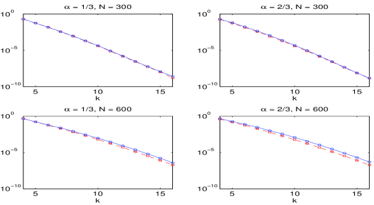
Figure 1: Error behavior of the Gauss-Jacobi rule for the approximation of $A_{1}^{\alpha-1}$ for $\tau=\tau^{\ast}$ (dashed line) and $\tau=\hat{\tau}=4k/N$ (solid line).

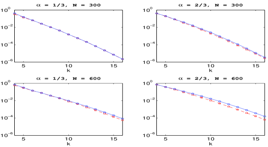
Figure 2: Error behavior of the Gauss-Jacobi rule for the approximation of $A_{3}^{\alpha-1}$ for $\tau=\tau^{\ast}$ (dashed line) and $\tau=\hat{\tau}=5k/N$ (solid line).

The previous results are all related to the overall error in the approximation of $A_{p}^{\alpha}.$ Considering that our final goal is the use of such approximation for the solution of FDEs, it is important to inspect also the componentwise error. As an example, in Figure 3, we report such errors, i.e., the values of $E_{j}$ defined in (3), in the case of $N=400,$ $p=1,$ $\tau=\hat{\tau}$ for $\alpha=0.3,0.5,0.7$, and different values of $k$. We also consider the componentwise errors of the polynomial approximation of the generating function obtained by truncating its Taylor series, with memory length equal to 16. Obviously this is equivalent to approximate with 0 the coefficients $\omega_{i}^{(p)}$ of (5), for $i>16$, so that the error is just $\left|\omega_{i}^{(p)}\right|$. The competitiveness of the rational approach is undeniable.

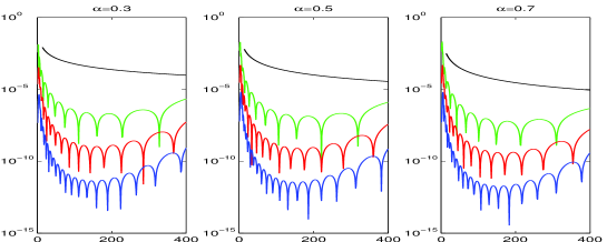
Figure 3: Componentwise error of the Gauss-Jacobi rational approximation with memory length $k=6,9,12$, and the polynomial approximation with $k=16$.

4 The solution of FDEs

In this section we discuss the use of the described approximation of $A_{1}^{\alpha}$ for getting a $k$-step method that simulates the FBDF of order 1. The discrete problem provided by the latter method applied for solving (1) can be written in matrix form as follows

$$\left(A_{1}^{\alpha}\otimes I_{s}\right)\left(Y-{\mathds{1}}\otimes y_{0}\right)=h^{\alpha}G(Y),$$ (36)

where $s$ is the dimension of the FDE, $I_{s}$ is the identity matrix of order $s,$ $y_{0}\in\mathbb{R}^{s}$ represents the initial value, $h=(T-t_{0})/N$ is the stepsize, ${\mathds{1}}=\left(1,1,\ldots,1\right)^{T}\in\mathbb{R}^{N},$

$$Y=\left(\begin{array}[]{c}y_{1}\\ y_{2}\\ \vdots\\ y_{N}\end{array}\right)\approx\left(\begin{array}[]{c}y(t_{1})\\ y(t_{2})\\ \vdots\\ y(t_{N})\end{array}\right),\qquad G(Y)=\left(\begin{array}[]{c}g(t_{1},y_{1})\\ g(t_{2},y_{2})\\ \vdots\\ g(t_{N},y_{N})\end{array}\right)\equiv\left(\begin{array}[]{c}g_{1}\\ g_{2}\\ \vdots\\ g_{N}\end{array}\right).$$

As described in Section 2, the use of a $k$-point Gauss-Jacobi rule for approximating (14) leads to

$$A_{1}^{\alpha}\approx\left(\begin{array}[]{ccccc}\beta_{0}&0&&&0\\ \vdots&\beta_{0}&0&&\\ \beta_{k}&\vdots&\ddots&0&\\ 0&\ddots&&\ddots&0\\ &0&\beta_{k}&\cdots&\beta_{0}\end{array}\right)^{-1}\left(\begin{array}[]{ccccc}\alpha_{0}&0&&&0\\ \vdots&\alpha_{0}&0&&\\ \alpha_{k}&\vdots&\ddots&0&\\ 0&\ddots&&\ddots&0\\ &0&\alpha_{k}&\cdots&\alpha_{0}\end{array}\right)\equiv B^{-1}C.$$

Here, the coefficients $\left\{\alpha_{j}\right\}_{j=0}^{k}$ and $\left\{\beta_{j}\right\}_{j=0}^{k}$ are related to the rational approximation through the formulas (16)–(18), with $m=k$ since $p=1,$

$$p_{k}(\zeta)=(1-\zeta)\widetilde{p}_{k-1}(1-\zeta)=\sum_{j=0}^{k}\alpha_{j}\zeta^{j},\qquad q_{k}(\zeta)=\widetilde{q}_{k}(1-\zeta)=\sum_{j=0}^{k}\beta_{j}\zeta^{j}.$$ (37)

If we replace $A_{1}^{\alpha}$ by $B^{-1}C$ in (36) and we multiply both side of the resulting equation from the left by $B\otimes I_{s},$ we obtain

$$\left(C\otimes I_{s}\right)Y-C{\mathds{1}}\otimes y_{0}=h^{\alpha}(B\otimes I_{s})G(Y),$$ (38)

where now $Y$ represents the numerical solution provided by the $k$-step method. In fact, considering that $(C{\mathds{1}})_{n}=0$ for each $n=k+1,\ldots,N,$ since

$$p_{k}(1)=\sum_{j=0}^{k}\alpha_{j}=0,$$ (39)

the discrete problem (38) simplifies to

$$\sum_{j=0}^{n-1}\alpha_{j}\left(y_{n-j}-y_{0}\right) = h^{\alpha}\sum_{j=0}^{n-1}\beta_{j}g_{n-j},\qquad n=1,\ldots,k,$$ (40)

$$\sum_{j=0}^{k}\alpha_{j}y_{n-j} = h^{\alpha}\sum_{j=0}^{k}\beta_{j}g_{n-j},\qquad n=k+1,\ldots,N.$$ (41)

Indeed, the equations in (40) allow to get an approximation of the solution over the first $k$ meshpoints which are then used as starting values for the $k$-step recursion in (41).

Remark 2

From (39)-(41) follows that the method reproduces exactly constant solutions, i.e. it is exact if $g(t,y(t))\equiv 0.$

As it happens in the case of ODEs, a localization of the zeros of the characteristic polynomials of the $k$-step method in (37) is required in order to study its stability properties. Clearly, such polynomials depend on the parameter $\tau,$ i.e. $p_{k}(\zeta)\equiv p_{k}(\zeta;\tau)$ and $q_{k}(\zeta)\equiv q_{k}(\zeta;\tau)$ since this dependence occurs in $\widetilde{p}_{k-1},\widetilde{q}_{k}.$ The method is therefore based on the following rational approximation

$$(1-\zeta)^{\alpha-1}\approx\frac{\widetilde{p}_{k-1}(1-\zeta;\tau)}{\widetilde{q}_{k}(1-\zeta;\tau)}\equiv\widetilde{R}_{k}(1-\zeta;\tau).$$ (42)

Theorem 3

For each $\tau\in(0,1],$ the adjoint of the characteristic polynomials of the $k$-step method, i.e. $\zeta^{k}p_{k}(\zeta^{-1};\tau)$ and $\zeta^{k}q_{k}(\zeta^{-1};\tau),$ are a Von Neumann and a Schur polynomial, respectively.

Proof. From Remark 1, one obtains

$$\widetilde{R}_{k}(1-\zeta;\tau)=\tau^{\alpha-1}\widetilde{R}_{k}\left(\frac{1-\zeta}{\tau};1\right),$$ (43)

since

$$\left.\frac{d^{l}}{d\zeta^{l}}(1-\zeta)^{\alpha-1}\right|_{\zeta=1-\tau}=\left.\tau^{\alpha-1}\frac{d^{l}}{d\zeta^{l}}\widetilde{R}_{k}\left(\frac{1-\zeta}{\tau};1\right)\right|_{\zeta=1-\tau},\qquad l=0,1,\ldots,2k-1.$$

In addition, using the Gauss hypergeometric functions, in [7, Theorem 4.1] it has been proved that

$$\widetilde{R}_{k}\left(\frac{1-\zeta}{\tau};1\right)=\frac{~{}_{2}F_{1}\left(1-k,1-\alpha-k;1-2k;(\tau-1+\zeta)/\tau\right)}{~{}_{2}F_{1}\left(-k,\alpha-k;1-2k;(\tau-1+\zeta)/\tau\right)},$$

or equivalently, by denoting with ${\mathcal{P}}_{r}^{(\gamma,\beta)}$ the Jacobi polynomial of degree $r$ and by using [15, eq. 142, p. 464] and the symmetry of such polynomials,

$$\widetilde{R}_{k}\left(\frac{1-\zeta}{\tau};1\right)=\tau\frac{(\tau-1+\zeta)^{k-1}{\mathcal{P}}_{k-1}^{(1-\alpha,\alpha)}\left(2\tau/(\tau-1+\zeta)-1\right)}{(\tau-1+\zeta)^{k}{\mathcal{P}}_{k}^{(\alpha-1,-\alpha)}\left(2\tau/(\tau-1+\zeta)-1\right)}.$$ (44)

From (37) and (42)–(44), one therefore gets

$$p_{k}(\zeta;\tau) = (1-\zeta)\tau^{\alpha}(\tau-1+\zeta)^{k-1}\mathcal{P}_{k-1}^{(1-\alpha,\alpha)}\left(2\tau/(\tau-1+\zeta)-1\right),$$

$$q_{k}(\zeta;\tau) = (\tau-1+\zeta)^{k}{\mathcal{P}}_{k}^{(\alpha-1,-\alpha)}\left(2\tau/(\tau-1+\zeta)-1\right).$$

It follows that, if we denote with $\theta_{i}$ the $i$th root of ${\mathcal{P}}_{k-1}^{(1-\alpha,\alpha)}$ then the roots of $p_{k}(\zeta;\tau)$ are given by

$$\zeta_{i}=1+\tau\frac{1-\theta_{i}}{1+\theta_{i}}>1,\quad i=1,\ldots,k-1,\qquad\zeta_{k}=1,$$ (45)

where the inequality follows from the fact that the roots of the Jacobi polynomials belong to $(-1,1).$ Similarly, by denoting with $\vartheta_{i}$ the $i$th root of ${\mathcal{P}}_{k}^{(\alpha-1,-\alpha)},$ one deduces that the roots of $q_{k}(\zeta;\tau)$ read

$$\zeta_{i}=1+\tau\frac{1-\vartheta_{i}}{1+\vartheta_{i}}>1,\quad i=1,\ldots,k.$$ (46)

From (45)-(46) the statement follows immediately.   

An important consequence of the previous result is that the finite recurrence scheme is always $0$-stable independently of the stepnumber $k$ and $\tau\in(0,1].$ More precisely, in the case of $g\equiv 0$ the zero solution of (41) is stable with respect to perturbations of the initial values.

4.1 Consistency

In this section we examine the consistency of the method. While, theoretically, it is only exact for constant solutions (see Remark 2), numerically one observes that the consistency is rather well simulated if $k$ is large enough. The analysis will also provide some hints about the choice of the memory length $m$. We restrict our consideration to the case $p=1$ ($m=k$) but the generalization is immediate.

For a given $y(t)$, the FBDF of order $1$ yields the approximation

$${}_{0}D_{t}^{\alpha}y(t)=\frac{1}{h^{\alpha}}\sum_{j=0}^{N}(-1)^{j}\binom{\alpha}{j}\left(y(t-jh)-y(0)\right)+O(h),\quad t=Nh.$$

Let

$$\Delta_{h}^{\alpha}y(t):=\sum_{j=0}^{N}(-1)^{j}\binom{\alpha}{j}\left(y(t-jh)-y(0)\right).$$

Writing a rational approximation of degree $k$ to $\omega_{1}^{(\alpha)}(\zeta)=\left(1-\zeta\right)^{\alpha}$ as

$$R_{k}(\zeta)=\sum_{j=0}^{\infty}\gamma_{j}\zeta^{j},$$

the corresponding method produces an approximation of the type

$${}_{0}D_{t}^{\alpha}y(t)\approx\frac{1}{h^{\alpha}}\sum_{j=0}^{N}\gamma_{j}\left(y(t-jh)-y(0)\right).$$

Denoting by

$$R_{k,h}^{\alpha}y(t):=\sum_{j=0}^{N}\gamma_{j}\left(y(t-jh)-y(0)\right),$$

we obtain

$${}_{0}D_{t}^{\alpha}y(t)-\frac{1}{h^{\alpha}}R_{k,h}^{\alpha}y(t)=$$

$$=~{}_{0}D_{t}^{\alpha}y(t)-\frac{1}{h^{\alpha}}\Delta_{h}^{\alpha}y(t)+\frac{1}{h^{\alpha}}\Delta_{h}^{\alpha}y(t)-\frac{1}{h^{\alpha}}R_{k,h}^{\alpha}y(t)$$

$$=O(h)+\frac{1}{h^{\alpha}}\sum\nolimits_{j=0}^{N}\left[(-1)^{j}\binom{\alpha}{j}-\gamma_{j}\right]\left(y(t-jh)-y(0)\right).$$

The consistency of the method is ensured if

$$\frac{1}{h^{\alpha}}\sum\nolimits_{j=0}^{N}\left[(-1)^{j}\binom{\alpha}{j}-\gamma_{j}\right]\left(y(t-jh)-y(0)\right)\rightarrow 0$$ (47)

as $h\rightarrow 0$ (cf. [6]). While this cannot be true for a fixed $k<\infty$, in what follows we show that numerically, i.e., for $h\geq h_{0}>0$, the consistency is well simulated if $k$ is large enough and if the rational approximation to $A_{p}^{\alpha}$ is reliable.

As pointed out in [12], a certain method for FDEs with generating function $\omega^{(\alpha)}(\zeta)$ is consistent of order $p$ if

$$h^{-\alpha}\omega^{(\alpha)}(e^{-h})=1+O(h^{p}).$$

In this setting, in order to understand the numerical consistence of our method, we consider the above relation by replacing $\omega^{(\alpha)}(e^{-h})$ with $\omega_{1}^{(\alpha)}(e^{-h})$ and $R_{k}(e^{-h})$. In particular, if we set

$$q_{k}(h)=\log_{h}\left(h^{-\alpha}\left|R_{k}(e^{-h})-\omega_{1}^{(\alpha)}(e^{-h})\right|\right),$$ (48)

then we obtain

$$h^{-\alpha}\left|R_{k}(e^{-h})\right| \leq h^{-\alpha}\left|\omega_{1}^{(\alpha)}(e^{-h})\right|+h^{-\alpha}\left|R_{k}(e^{-h})-\omega_{1}^{(\alpha)}(e^{-h})\right|.$$

$$= 1+O(h)+h^{q_{k}(h)}$$

This implies that the consistency of the FBDF of the first order is well simulated as long as $q_{k}(h)$ is larger than $1.$ In Figure 4, we plot such function for $\alpha=1/2,$ $\tau=1/10$, and different values of $k.$

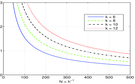
Figure 4: Plot of the function $q_{k}(h)$ in (48) for $\alpha=1/2,$ $\tau=1/10$ and different values of $k.$

The previous experiment does not take care of the perturbation introduced in the approximation of the fractional derivative of fractional powers of the independent variable which may be present in the solution of the FDE. In order to control such perturbations, we therefore consider the following second experiment. Going back to formula (47), we let $N=1/h$ and $y(t)=E_{\alpha}(-t^{\alpha})$ where $E_{\alpha}(x)$ denotes the one-parameter Mittag-Leffler function (see e.g. [16, Chapter 1])

$$E_{\alpha}(x)=\sum_{k=0}^{\infty}\frac{x^{k}}{\Gamma(k\alpha+1)}.$$ (49)

In Figure 5, we then consider the behavior of the function

$$\widetilde{q}_{k}(h)=\log_{h}\left(h^{-\alpha}\left|\sum\nolimits_{j=0}^{N}\left((-1)^{j}\left(\begin{array}[]{c}\alpha\\ j\end{array}\right)-\gamma_{j,k}\right)(y(t_{N-j})-y(0))\right|\right)$$ (50)

which, similarly to $q_{k}(h),$ has to be compared with $1.$ The values of $y(t)$ have been computed using the Matlab function mlf from [17] that implements the Mittag-Leffler function together with the Schur-Parlett algorithm.

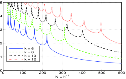
Figure 5: Plot of the function $\widetilde{q}_{k}(h)$ in (50) for $\alpha=1/2,$ $\tau=1/10$ and different values of $k.$

We conclude this section by considering what happens with the general assumption $\left|y(t)\right|\leq M$. Using this bound, by (47) we consider the function

$$\overline{q}_{k}(h)=\log_{h}\left(h^{-\alpha}\sum\nolimits_{j=0}^{N}\left|(-1)^{j}\binom{\alpha}{j}-\gamma_{j,k}\right|\right),$$ (51)

whose behavior is reported in Figure 6.

As already mentioned, the numerical analysis reported in this section can also be used to select a proper value for $k$ for a fixed time stepping $h$ or viceversa. Figures 4 and 6 are in fact independent of the problem and can be used easily to this aim.

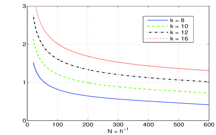
Figure 6: Plot of the function $\bar{q}_{k}(h)$ in (51), for $\alpha=1/2,$ $\tau=1/10$ and different values of $k.$

4.2 Linear stability

For what concerns the linear stability, taking $g(t,y(t))=\lambda y(t)$ in (1), we have that $y(t)=E_{\alpha}(\lambda t^{\alpha})\rightarrow 0$ for

$$\left|\arg(\lambda)-\pi\right|<\left(1-\frac{\alpha}{2}\right)\pi,$$

(see (49) and [13]). The absolute stability region of a FBDF is given by the complement of $\left\{\omega_{p}^{(\alpha)}(\zeta):\left|\zeta\right|\leq 1\right\}$ so that a good approximation of the generating function should lead to similar stability domains and hence good stability properties. We consider the behavior of methods based on the Gauss-Jacobi rule whose corresponding stability regions are given by, see (17)-(18),

$$\mathbb{C}\backslash\left\{\frac{p_{m}(\zeta)}{q_{m}(\zeta)}:\left|\zeta\right|\leq 1\right\}.$$

From a theoretical point of view, from Theorem 3 one deduces that for $p=1$ such regions are always unbounded for each $m=k$ and $\tau\in(0,1].$ Indeed, as shown in Figure 7, the methods simulate the behavior of the FBDFs rapidly, i.e. already for $k$ and therefore $m$ small. In particular, the stability domain of the method of degree $k=m=12$ in the left frame of Figure 7 is very close to the one of the FBDF of order $1.$

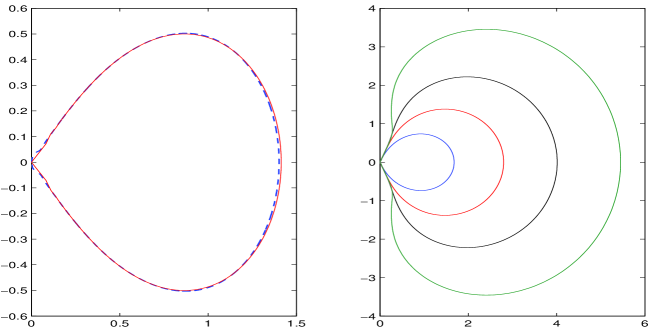
Figure 7: Left: boundary of the stability domains of the methods based on the Gauss-Jacobi rule with $k=6$ (dashed line) and $k=12$ (solid line) for $p=1,$ $\tau=1/10,$ and $\alpha=1/2$. Right: boundary of the stability domains of the same methods of degree $k=8$ for $p=1$ (inner) to $4$ (outer), $\tau=1/10$ and $\alpha=3/4$.

5 Numerical examples

As first example, we consider the one-dimensional Nigmatullin’s type equation

$${}_{0}D_{t}^{\alpha}u(x,t) = \frac{\partial^{2}u(x,t)}{\partial x^{2}},\quad t>0,\quad x\in\left(0,\pi\right),$$

$$u(0,t) = u(\pi,t)=0,$$

$$u(x,0) = \sin x.$$

If we discretize the spatial derivative by applying the classical central differences on a uniform mesh of meshsize $\delta=\pi/(s+1),$ we obtain the $s$-dimensional FDE

$${}_{0}D_{t}^{\alpha}y(t)=Ly(t),\quad y(0)=y_{0},$$ (52)

where $L=\delta^{-2}\cdot\mbox{tridiag}(1,-2,1)$, and $y_{0}$ is the sine function evaluated at the interior grid points. It is known that $y_{0}$ is the eigenvector of $L$ corresponding to its largest eigenvalue $\lambda=-4\sin^{2}(\delta/2)/\delta^{2}.$ This implies that the exact solution of (52) is given by, see (49),

$$y(t)=E_{\alpha}(t^{\alpha}\lambda)y_{0}.$$

In Figure 8 some results are reported. We compare the maximum norm of the error at each step of the FBDF of order 1 (FBDF1) and the method based on the Gauss-Jacobi rule for some values of $k$ and $\alpha.$ The initial values for the $k$-step schemes are defined according to the strategy described in Section 4. The reference solutions have been computed using the already mentioned Matlab function mlf from [17]. The dimension of the problem is $s=50$, and we consider a uniform time step $h=1/N$ with $N=250$ so that $h\approx\delta^{2}$. As one can see, if we set $\tau=1$, i.e. if we use the classical Padè approximation of $(1-\zeta)^{\alpha-1}$ (see Remark 1), the $k$-step methods simulate quite well the FBDF1 initially and an improvement of the results can be obtained by slightly increasing (considering to the total number of integration steps) the stepnumber $k.$ A noticeable improvement can be obtained by choosing a different value of $\tau.$ In particular, if we set $\tau={\hat{\tau}}=4k/N$ (see (35)) then the $6$-step method provides a numerical solution with the same accuracy of the one provided by the FBDF1 over the entire integration interval.

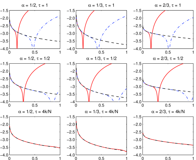
Figure 8: Step by step error (in logarithmic scale) for the solution of (52) for the FBDF of order 1 (dashed line) and the method based on the Gauss-Jacobi rule with $k=6$ (solid line) and $k=12$ (dash-dotted line).

As second example we consider the following nonlinear problem

$${}_{0}D_{t}^{\alpha}u(x,t) = \frac{\partial(p(x)u(x,t))}{\partial x}+K_{\alpha}\frac{\partial^{2}u(x,t)}{\partial x^{2}}+ru(x,t)\left(1-\frac{u(x,t)}{K}\right),$$

$$u(0,t) = u(5,t)=0,\quad t\in[0,1],$$

$$u(x,0) = x^{2}(5-x)^{2},\quad x\in[0,5].$$

This is a particular instance of the time fractional Fokker-Planck equation with a nonlinear source term [18]. In population biology, its solution $u(x,t)$ represents the population density at location $x$ and time $t$ and the nonlinear source term in the equation is known as Fisher’s growth term.

The application of the classical second order semi-discretization in space with stepsize $\delta=5/(s+1)$ leads to the following initial value problem

$${}_{0}D_{t}^{\alpha}y(t)=Jy(t)+g(y(t)),\quad t\in(0,1],\qquad y(0)=y_{0},$$ (53)

where, for each $i=1,\ldots,s,$ $(y(t))_{i}\equiv y_{i}(t)\approx u(i\delta,t),$ $y_{i}(0)=u(i\delta,0),$ $(g(y))_{i}=ry_{i}(1-y_{i}/K),$ and $J$ is a tridiagonal matrix whose significant entries are

$$J_{ii} = p^{\prime}(x_{i})-\frac{2K_{\alpha}}{\delta^{2}},\qquad i=1,\ldots,s,$$

$$J_{i,i-1} = -\frac{p(x_{i})}{2\delta}+\frac{K_{\alpha}}{\delta^{2}},\quad J_{i-1,i}=\frac{p(x_{i-1})}{2\delta}+\frac{K_{\alpha}}{\delta^{2}},\qquad i=1,\ldots,s-1.$$

In our experiment, we set $\alpha=0.8,$ $p(x)=-1,$ $r=0.2,$ $K_{\alpha}=K=1$ (see [18, Example 5.4]) and $s=90.$ We solved (53) over a uniform meshgrid with stepsize $h=1/256$ by using the FBDF1 and the $6$-step method with $\tau=24/256.$ The so-obtained numerical solutions have the same qualitative behavior as shown in Figure 9 for different times $t=1/8,1/2,1.$ This is confirmed by the step by step maximum norm of the difference between them reported in Figure 10.

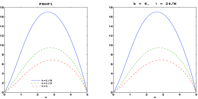
Figure 9: Numerical solution of (53) with $\alpha=0.8$ provided by the FBDF1 and the method based on the Gauss-Jacobi rule with $k=6$ at $t=1/8,1/2,1.$

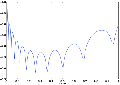
Figure 10: Step by step norm of the difference (in logarithmic scale) between the numerical solutions provided by the FBDF1 and the $6$-step methods.

6 Conclusion

In this paper we have presented a new approach for the construction of $m$-step formulas for the solution of FDEs. The method shows encouraging results in the discrete approximation of the FDE solution especially if we consider the computational saving with respect to the attainable accuracy. Indeed good results are attainable with short memory length. Theoretically the method is $0$-stable and the consistency is well simulated. The linear stability is preserved.

We finally remark that even if the paper only deals with the approximation of FBDFs, the ideas can easily be extended to other approaches such as the Fractional Adams type methods. It is just necessary to detect the generating function or the corresponding Toeplitz matrix and then apply the technique presented in the paper.

References

[1] D.A. Bini, N.J. Higham, B. Meini, Algorithms for the matrix
pth root, Numer. Algorithms 39 (2005), 349–378.
[2] H. Brunner, P.J. van der Houwen, The numerical solution of
Volterra equations. CWI Monographs, 3. North-Holland Publishing Co.,
Amsterdam, 1986.
[3] K. Diethelm, N.J. Ford, Analysis of fractional differential
equations, J. Math. Anal. Appl. 265 (2002), 229–248.
[4] K. Diethelm, J.M. Ford, N.J. Ford, M. Weilbeer, Pitfalls in
fast numerical solvers for fractional differential equations, J. Comput.
Appl. Math. 186 (2006), 482–503.
[5] A. Frommer, S. Güttel, M. Schweitzer, Efficient and stable
Arnoldi restarts for matrix functions based on quadrature, Preprint
BUW-IMACM 13/17 (2013) http://www.math.uni-wuppertal.de.
[6] L. Galeone, R. Garrappa, On multistep methods for differential
equations of fractional order, Mediterr. J. Math. 3 (2006), 565-580.
[7] O. Gomilko, F. Greco, K. Ziȩtak, A Padé family of
iterations for the matrix sign function and related problems, Numerical
Linear Algebra with Applications 19 (2012), 585–605.
[8] E. Hairer, S.P. Norsett, G. Wanner, Solving ordinary
differential equations. I. Nonstiff problems. Second edition. Springer
Series in Computational Mathematics, 8. Springer-Verlag, Berlin, 1993.
[9] N. Hale, N.J. Higham, L.N. Trefethen, Computing ,
, and related matrix functions by contour integrals, SIAM J. Numer.
Anal. 46 (2008), 2505–2523.
[10] N.J. Higham, Functions of matrices. Theory and computation.
Society for Industrial and Applied Mathematics (SIAM), Philadelphia, PA,
2008.
[11] F.B. Hildebrand, Introduction to Numerical Analysis. New York:
McGraw-Hill, 1956.
[12] C. Lubich, Discretized fractional calculus, SlAM J. Math.
Anal. 17 (1986), 704–719.
[13] C. Lubich, A stability analysis of convolution quadratures
for Abel-Volterra integral equations, IMA J. Numer. Anal. 6 (1986), 87–101.
[14] P. Novati, Numerical approximation to the fractional
derivative operator, to appear in Numerische Mathematik, 2013, DOI:
10.1007/s00211-013-0596-7.
[15] A.P.Prudnikov, Yu.A. Brychkov, O.I. Marichev, Integrals and
Series, vol.3: More Special Functions, Gordon and Breach Science Publishers,
1990.
[16] I. Podlubny, Fractional differential equations. Mathematics in
Science and Engineering, 198. Academic Press, Inc., San Diego, CA, 1999.
[17] I. Podlubny, Mittag–Leffler Function,
http://www.mathworks.com/matlabcentral/fileexchange/8738, 2009.
[18] Q. Yang, F. Liu, I. Turner, Stability and convergence of an
effective numerical method for the Time-Space Fractional Fokker-Planck
Equation with a nonlinear source term, Int. J. Differ. Equ. (2010), Art. ID
464321, 22 pp.