Discussion of Big Bayes Stories and BayesBag

1 Introductory Remarks

I congratulate all the authors for their insightful papers with wide-ranging contributions. The articles demonstrate the power and elegance of the Bayesian inference paradigm. In particular, it allows to incorporate prior knowledge as well as hierarchical model building in a convincing way. Regarding the latter, the contribution by Raftery, Alkema and German is a very fascinating piece, as it addresses a set of problems of great public interest and presents predictions for the world populations and other interesting quantities with uncertainty regions. Their approach is based on a hierarchical model, taking various characteristics into account (e.g., fertility projections). It would have been very difficult to come up with a “better” solution which would be as clear in terms of interpretation (in contrast to a “black-box machine”) and which would provide (model-based) uncertainties for the predictions into the future.

2 Uncertainty, Stability and Bagging the Posterior

Many of the papers quantify in one or another form various notions of uncertainties. In the Bayesian framework, this is usually based on the posterior distribution. An old “debate” is how much the results are sensitive to the choice of the prior, and I believe that some reasonable sensitivity analysis can lead to much insight. The sensitivity with respect to “perturbed data” though is not easily captured by the Bayesian framework. In the context of prediction, Leo Breiman (Breiman, 1996a, 1996b) has pointed to issues of stability with respect to perturbations of the data, Bousquet and Elisseeff (2002) provide some mathematical connections to prediction performance while Meinshausen and Bühlmann (2010) present some theory and methodology for controlling the frequentist error of expected false positives.

As an example, the (frequentist) Lasso (Tibshirani, 1996) is very unstable for estimating the unknown parameters in a linear model, in particular, if the correlation among the covariates is high (for two highly correlated variables where at least one of them has a substantially large regression coefficient, the Lasso selects either one or the other in an unstable fashion). Thus, the MAP for a Gaussian linear model with a Double-Exponential prior for the regression coefficients is unstable. The posterior distribution is probably more stable but, presumably, it is still “rather” sensitive with respect to perturbation of the data: if the data would look a bit different, the posterior might be “rather” different. The situation becomes more exposed to stability problems when using spike and slab priors (Mitchell and Beauchamp, 1988), due to increased sparsity.

We can stabilize the posterior distribution by using a bootstrap and aggregation scheme, in the spirit of bagging (Breiman, 1996b). In a nutshell, denote by $\mathcal{D}^{*}$ a bootstrap- or subsample of the data $\mathcal{D}$. The posterior of the random parameters $\theta$ given the data $\mathcal{D}$ has c.d.f. $F(\cdot|\mathcal{D})$, and we can stabilize this using

$$F_{\mathrm{BayesBag}}(\cdot|\mathcal{D})=\mathbb{E}^{*}\bigl{[}F\bigl{(}\cdot|\mathcal{D}^{*}\bigr{)}\bigr{]},$$

where $\mathbb{E}^{*}$ is with respect to the bootstrap- or subsampling scheme. We call it the BayesBag estimator. It can be approximated by averaging over $B$ posterior computations for bootstrap- or subsamples, which might be a rather demanding task (although say $B=10$ would already stabilize to a certain extent). Note that when conditioning on the data, the posterior $F(\cdot|\mathcal{D})$ is a fixed c.d.f., but when taking the view point that the data could change, it is useful to consider randomized perturbed versions $F(\cdot|\mathcal{D}^{*})$ which are to be aggregated.

=9.7cm Sample size $\bm{(2.5\%,97.5\%)}$ posterior $\bm{(2.5\%,97.5\%)}\ \bm{\mathit{BayesBag}}$ $n=1$ $(-0.69,2.81)$ $(-1.30,3.41)$ $n=10$ $(0.10,1.32)$ $(-0.16,1.56)$

Table 1: 2.5% and 97.5% quantiles of the posterior $F(\cdot|\overline{X}_{n})$ in (2) andof the BayesBag (bagged posterior) in (2). The data wasgenerated once using a single realized value of $\theta=1.31$

The following simple and rather stable example shows that such a bagging scheme outputs a larger uncertainty which is perhaps more appropriate.

Consider the model

$$\begin{array}[]{r@{\quad}l}&\theta\sim\mathcal{N}\bigl{(}0,\tau^{2}\bigr{)},\\[2.0pt] \mbox{conditional on }\theta{:}&X_{1},\ldots,X_{n}\,\mathrm{i.i.d.}\sim\mathcal{N}\bigl{(}\theta,\sigma^{2}\bigr{)}.\end{array}$$

It is well known that the posterior distribution equals

$$\theta|\overline{X}_{n}\sim\mathcal{N}\biggl{(}\frac{\sum_{i=1}^{n}X_{i}}{n+\sigma^{2}/\tau^{2}},\biggl{(}\frac{1}{\tau^{2}}+\frac{n}{\sigma^{2}}\biggr{)}^{-1}\biggr{)}.$$

Denote by $F(\cdot;\overline{X}_{n})$ the c.d.f. of the posterior distribution, that is,

$$F(u;\overline{X}_{n})=\Phi\biggl{(}u,\mathrm{mean}=\frac{n\overline{X}_{n}}{n+\sigma^{2}/\tau^{2}},$$

(1)

$$\phantom{\hskip 80.0pt}\mathrm{var}=\biggl{(}\frac{1}{\tau^{2}}+\frac{n}{\sigma^{2}}\biggr{)}^{-1}\biggr{)},$$

where $\Phi(u,\mathrm{mean}=m,\mathrm{var}=s^{2})=\Phi((u-m)/s)$ and $\Phi(\cdot)$ denotes the c.d.f. of $\mathcal{N}(0,1)$. We can either use the nonparametric bootstrap, with resampling the data with replacement, or a parametric bootstrap (assuming here that $\sigma^{2}$ is known):

$$X_{1}^{*},\ldots,X_{n}^{*}\,\mathrm{i.i.d.}\,\mathcal{N}\bigl{(}\hat{\theta},\sigma^{2}\bigr{)},\quad\hat{\theta}=\overline{X}_{n}.$$ (2)

With the parametric bootstrap in (2), we can easily calculate the BayesBag estimator:

$$\mathbb{E}^{*}\bigl{[}F\bigl{(}u;\overline{X}_{n}^{*}\bigr{)}\bigr{]}$$

$$\quad=\int\Phi\biggl{(}\frac{u-r}{\sqrt{({1}/{\tau^{2}}+{n}/{\sigma^{2}})^{-1}}}\biggr{)}$$

(3)

$$\phantom{\quad=\int}{}\cdot\varphi\biggl{(}r,\mathrm{mean}=\frac{n\overline{X}_{n}}{n+\sigma^{2}/\tau^{2}},$$

$$\phantom{\hskip 62.0pt}\mathrm{var}=\frac{n\sigma^{2}}{(n+\sigma^{2}/\tau^{2})^{2}}\biggr{)}\,dr,$$

where $\varphi(r,\mathrm{mean}=m,\mathrm{var}=s^{2})=s^{-1}\varphi((r-m)/s)$ and $\varphi(\cdot)$ denotes the p.d.f. of $\mathcal{N}(0,1)$. We consider the posterior credible region by computing the 2.5% and 97.5% quantiles of $F(\cdot;\overline{X}_{n})$ and we compare these quantiles with the corresponding ones from the BayesBag $\mathbb{E}^{*}[F(\cdot;\overline{X}_{n}^{*})]$ above in (2). We only consider here the case with $\sigma^{2}=1$ and $\tau^{2}=4$, and the results are given in Table 1. Of course, we can also look at the variability of the posterior via the bootstrapped c.d.f.’s $F(\cdot|\overline{X}_{n}^{*})$, instead of considering the bootstrap mean (BayesBag) only. Figure 1 illustrates that variability can be rather high, but the situation obviously improves as sample size increases.

It is worth pointing out that, in general, one could use a parametric bootstrap when using $\hat{\theta}$ as the MAP of the posterior distribution, and such a scheme could be used in models with complex hierarchical and dependence structures.

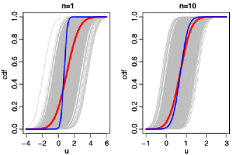
Figure 1: 1000 bootstrapped cumulative distribution functions $F(u|\overline{X}_{n}^{*})$ of $\theta|\overline{X}_{n}^{*}$. The BayesBag (i.e., mean) $\mathbb{E}^{*}[F(u|\overline{X}_{n}^{*})]$ in (2) (thick red line) and the cumulative distribution function $F(u|\overline{X}_{n})$ of the classical posterior of $\theta|\overline{X}_{n}$ in (2) (blue line). Left panel for $n=1$ and right panel for $n=10$, and note the different scales for the x-axis. The data is as in Table 1.

The frequentist approach usually does not address stability issues either and, in addition, assigning $p$-values and confidence intervals in complex scenarios is a nontrivial problem. Recent progress has been achieved for high-dimensional sparse models (Minnier, Tian and Cai (2011); Zhang and Zhang (2014); Bogdan et al. (2013); Bühlmann (2013); van de Geer et al. (2014), cf.); regarding the issue of constructing “stable $p$-values,” an approach based on subsampling and appropriate aggregation of $p$-values is described in Meinshausen, Meier and Bühlmann (2009). Yet, much more work in frequentist inference would be needed to cope with, for example, high-dimensional hierarchical models in non-i.i.d. settings such as space–time processes or clustered data, or, as another example, the population dynamic model in the beautiful paper by Kuikka, Vanhatalo, Pulkkinen, Mäntyniemi and Corander in this issue.

3 Networks and Graphical Models

The paper by Johnson, Abal, Ahern an Hamilton presents an interesting application by using Bayesian inference for a Bayesian network (as is well known, the term “Bayesian network” does not require Bayesian inference at all—and it is somewhat confusing). The arrows in the directed acyclic graph often indicate causal relations (Pearl (2000); Spirtes, Glymour and Scheines (2000)) and, as such, the model allows for causal conclusions. Great care is needed, of course, when the DAG is misspecified or estimated from observational data since causal conclusions are depending in a very “sensitive way” on the underlying DAG. A lot of work exists regarding identifiability of the DAG from observational data (Pearl (2000); Spirtes, Glymour and Scheines (2000); Shpitser and Pearl (2008); Hoyer et al. (2009); Peters and Bühlmann (2014), cf.), and, obviously, there are ill-posed situations such as with a bivariate Gaussian distribution where one cannot identify the causal direction between two variables. In the Bayesian framework, the problem of identifiability does not exist in a “direct sense”: but I believe it must come in through another channel, presumably by a high sensitivity with respect to prior specifications. Due to severe identifiability problems, causal inference based on observational data is ill-posed or depends on nontestable assumptions. However, one can nevertheless (under some assumptions) derive lower bounds on absolute values of causal effects (Maathuis, Kalisch and Bühlmann, 2009). As lower bounds, they are conservative and a Bayesian average bound would be interesting.

In view of nontestable assumptions, causal models should be validated with randomized experiments. Often though, this cannot be done due to limited resources or ethical reasons. The field of molecular biology with simple organisms is an interesting application where causal model validation is feasible thanks to gene knock-out or other manipulation methods. We pursued this in the past, for estimated causal structures and models based on frequentist approaches, for the organisms yeast (Maathuis et al., 2010) and arabidopsis thaliana (Stekhoven et al., 2012). These two papers indicate that it is indeed possible to predict to a certain extent lower bounds of causal strength and relations based on observational (and very high-dimensional) data. Such a conclusion can only be made post-hoc, after validation—and validation has nothing to do whether a Bayesian or any other inference machine has been used.

References

- Bogdan et al. (2013) {bmisc}[auto:STB—2014/02/12—12:18:25] \bauthor\bsnmBogdan, \bfnmM.\binitsM., \bauthor\bsnmvan den Berg, \bfnmE.\binitsE., \bauthor\bsnmSu, \bfnmW.\binitsW. and \bauthor\bsnmCandès, \bfnmE.\binitsE. (\byear2013). \bhowpublishedStatistical estimation and testing via the sorted L1 norm. Available at \arxivurlarXiv:1310.1969. \bptokimsref\endbibitem
- Bousquet and Elisseeff (2002) {barticle}[mr] \bauthor\bsnmBousquet, \bfnmOlivier\binitsO. and \bauthor\bsnmElisseeff, \bfnmAndré\binitsA. (\byear2002). \btitleStability and generalization. \bjournalJ. Mach. Learn. Res. \bvolume2 \bpages499–526. \biddoi=10.1162/153244302760200704, issn=1532-4435, mr=1929416 \bptokimsref\endbibitem
- Breiman (1996a) {barticle}[auto:STB—2014/02/12—12:18:25] \bauthor\bsnmBreiman, \bfnmL.\binitsL. (\byear1996a). \btitleBagging predictors. \bjournalMach. Learn. \bvolume24 \bpages123–140. \bptokimsref\endbibitem
- Breiman (1996b) {barticle}[mr] \bauthor\bsnmBreiman, \bfnmLeo\binitsL. (\byear1996b). \btitleHeuristics of instability and stabilization in model selection. \bjournalAnn. Statist. \bvolume24 \bpages2350–2383. \biddoi=10.1214/aos/1032181158, issn=0090-5364, mr=1425957 \bptokimsref\endbibitem
- Bühlmann (2013) {barticle}[auto:STB—2014/02/12—12:18:25] \bauthor\bsnmBühlmann, \bfnmP.\binitsP. (\byear2013). \btitleStatistical significance in high-dimensional linear models. \bjournalBernoulli \bvolume19 \bpages1212–1242. \bptokimsref\endbibitem
- Hoyer et al. (2009) {bincollection}[auto:STB—2014/02/12—12:18:25] \bauthor\bsnmHoyer, \bfnmP.\binitsP., \bauthor\bsnmJanzing, \bfnmD.\binitsD., \bauthor\bsnmMooij, \bfnmJ.\binitsJ., \bauthor\bsnmPeters, \bfnmJ.\binitsJ. and \bauthor\bsnmSchölkopf, \bfnmB.\binitsB. (\byear2009). \btitleNonlinear causal discovery with additive noise models. In \bbooktitleAdvances in Neural Information Processing Systems 21 \bpages689–696. \bpublisherCurran Associates, \baddressRed Hook, NY. \bptokimsref\endbibitem
- Maathuis et al. (2010) {barticle}[pbm] \bauthor\bsnmMaathuis, \bfnmMarloes H.\binitsM. H., \bauthor\bsnmColombo, \bfnmDiego\binitsD., \bauthor\bsnmKalisch, \bfnmMarkus\binitsM. and \bauthor\bsnmBühlmann, \bfnmPeter\binitsP. (\byear2010). \btitlePredicting causal effects in large-scale systems from observational data. \bjournalNat. Methods \bvolume7 \bpages247–248. \biddoi=10.1038/nmeth0410-247, issn=1548-7105, pii=nmeth0410-247, pmid=20354511 \bptokimsref\endbibitem
- Maathuis, Kalisch and Bühlmann (2009) {barticle}[mr] \bauthor\bsnmMaathuis, \bfnmMarloes H.\binitsM. H., \bauthor\bsnmKalisch, \bfnmMarkus\binitsM. and \bauthor\bsnmBühlmann, \bfnmPeter\binitsP. (\byear2009). \btitleEstimating high-dimensional intervention effects from observational data. \bjournalAnn. Statist. \bvolume37 \bpages3133–3164. \biddoi=10.1214/09-AOS685, issn=0090-5364, mr=2549555 \bptokimsref\endbibitem
- Meinshausen and Bühlmann (2010) {barticle}[mr] \bauthor\bsnmMeinshausen, \bfnmNicolai\binitsN. and \bauthor\bsnmBühlmann, \bfnmPeter\binitsP. (\byear2010). \btitleStability selection. \bjournalJ. R. Stat. Soc. Ser. B Stat. Methodol. \bvolume72 \bpages417–473. \biddoi=10.1111/j.1467-9868.2010.00740.x, issn=1369-7412, mr=2758523 \bptnotecheck related \bptokimsref\endbibitem
- Meinshausen, Meier and Bühlmann (2009) {barticle}[mr] \bauthor\bsnmMeinshausen, \bfnmNicolai\binitsN., \bauthor\bsnmMeier, \bfnmLukas\binitsL. and \bauthor\bsnmBühlmann, \bfnmPeter\binitsP. (\byear2009). \btitle-values for high-dimensional regression. \bjournalJ. Amer. Statist. Assoc. \bvolume104 \bpages1671–1681. \biddoi=10.1198/jasa.2009.tm08647, issn=0162-1459, mr=2750584 \bptokimsref\endbibitem
- Minnier, Tian and Cai (2011) {barticle}[mr] \bauthor\bsnmMinnier, \bfnmJessica\binitsJ., \bauthor\bsnmTian, \bfnmLu\binitsL. and \bauthor\bsnmCai, \bfnmTianxi\binitsT. (\byear2011). \btitleA perturbation method for inference on regularized regression estimates. \bjournalJ. Amer. Statist. Assoc. \bvolume106 \bpages1371–1382. \biddoi=10.1198/jasa.2011.tm10382, issn=0162-1459, mr=2896842 \bptokimsref\endbibitem
- Mitchell and Beauchamp (1988) {barticle}[mr] \bauthor\bsnmMitchell, \bfnmT. J.\binitsT. J. and \bauthor\bsnmBeauchamp, \bfnmJ. J.\binitsJ. J. (\byear1988). \btitleBayesian variable selection in linear regression. \bjournalJ. Amer. Statist. Assoc. \bvolume83 \bpages1023–1036. \bidissn=0162-1459, mr=0997578 \bptnotecheck related \bptokimsref\endbibitem
- Pearl (2000) {bbook}[mr] \bauthor\bsnmPearl, \bfnmJudea\binitsJ. (\byear2000). \btitleCausality: Models, Reasoning, and Inference. \bpublisherCambridge Univ. Press, \blocationCambridge. \bidmr=1744773 \bptokimsref\endbibitem
- Peters and Bühlmann (2014) {barticle}[auto:STB—2014/02/12—12:18:25] \bauthor\bsnmPeters, \bfnmJ.\binitsJ. and \bauthor\bsnmBühlmann, \bfnmP.\binitsP. (\byear2014). \btitleIdentifiability of Gaussian structural equation models with equal error variances. \bjournalBiometrika \bvolume101 \bpages219–228. \bptokimsref\endbibitem
- Shpitser and Pearl (2008) {barticle}[mr] \bauthor\bsnmShpitser, \bfnmIlya\binitsI. and \bauthor\bsnmPearl, \bfnmJudea\binitsJ. (\byear2008). \btitleComplete identification methods for the causal hierarchy. \bjournalJ. Mach. Learn. Res. \bvolume9 \bpages1941–1979. \bidissn=1532-4435, mr=2447308 \bptokimsref\endbibitem
- Spirtes, Glymour and Scheines (2000) {bbook}[auto:STB—2014/02/12—12:18:25] \bauthor\bsnmSpirtes, \bfnmP.\binitsP., \bauthor\bsnmGlymour, \bfnmC.\binitsC. and \bauthor\bsnmScheines, \bfnmR.\binitsR. (\byear2000). \btitleCausation, Prediction, and Search, \bedition2nd ed. \bpublisherMIT Press, \blocationCambridge, MA. \bptokimsref\endbibitem
- Stekhoven et al. (2012) {barticle}[pbm] \bauthor\bsnmStekhoven, \bfnmDaniel J.\binitsD. J., \bauthor\bsnmMoraes, \bfnmIzabel\binitsI., \bauthor\bsnmSveinbjörnsson, \bfnmGardar\binitsG., \bauthor\bsnmHennig, \bfnmLars\binitsL., \bauthor\bsnmMaathuis, \bfnmMarloes H.\binitsM. H. and \bauthor\bsnmBühlmann, \bfnmPeter\binitsP. (\byear2012). \btitleCausal stability ranking. \bjournalBioinformatics \bvolume28 \bpages2819–2823. \biddoi=10.1093/bioinformatics/bts523, issn=1367-4811, pii=bts523, pmid=22945788 \bptokimsref\endbibitem
- Tibshirani (1996) {barticle}[mr] \bauthor\bsnmTibshirani, \bfnmRobert\binitsR. (\byear1996). \btitleRegression shrinkage and selection via the lasso. \bjournalJ. Roy. Statist. Soc. Ser. B \bvolume58 \bpages267–288. \bidissn=0035-9246, mr=1379242 \bptokimsref\endbibitem
- van de Geer et al. (2014) {bmisc}[auto:STB—2014/02/12—12:18:25] \bauthor\bsnmvan de Geer, \bfnmS.\binitsS., \bauthor\bsnmBühlmann, \bfnmP.\binitsP., \bauthor\bsnmRitov, \bfnmY.\binitsY. and \bauthor\bsnmDezeure, \bfnmR.\binitsR. (\byear2014). \bhowpublishedOn asymptotically optimal confidence regions and tests for high-dimensional models. Ann. Statist. To appear. Available at \arxivurlarXiv:1303.0518. \bptokimsref\endbibitem
- Zhang and Zhang (2014) {barticle}[auto:STB—2014/02/12—12:18:25] \bauthor\bsnmZhang, \bfnmC.-H.\binitsC.-H. and \bauthor\bsnmZhang, \bfnmS.\binitsS. (\byear2014). \btitleConfidence intervals for low dimensional parameters in high dimensional linear models. \bjournalJ. R. Stat. Soc. Ser. B. Stat. Methodol. \bvolume76 \bpages217–242. \bidmr=3153940 \bptokimsref\endbibitem