Galaxy Formation: Bayesian History Matching for the Observable Universe

Abstract

Cosmologists at the Institute of Computational Cosmology, Durham University, have developed a state of the art model of galaxy formation known as Galform, intended to contribute to our understanding of the formation, growth and subsequent evolution of galaxies in the presence of dark matter. Galform requires the specification of many input parameters and takes a significant time to complete one simulation, making comparison between the model’s output and real observations of the Universe extremely challenging. This paper concerns the analysis of this problem using Bayesian emulation within an iterative history matching strategy, and represents the most detailed uncertainty analysis of a galaxy formation simulation yet performed.

, and

1 Introduction

Understanding the evolution of the universe from the Big Bang to the current day is the fundamental goal of cosmology. A major part of this is the problem of structure formation: understanding the formation, growth and subsequent evolution of galaxies in the presence of dark matter. The world leading Galform group, based at the Institute of Computational Cosmology, Durham University, has developed a state of the art model of galaxy formation know as Galform. However, they face a critical problem. Galform requires the specification of many input parameters and takes a significant time to complete one simulation, making comparison between the model’s output and real observations of the universe extremely challenging.

Here we describe the analysis of this problem using Bayesian history matching methodology, highlighting why the problem itself can only be sensibly formulated within a subjective Bayesian context and demonstrating the use of Bayesian emulators within an iterative history matching strategy. This work represents the most detailed uncertainty analysis of a galaxy formation simulation yet performed and, to our knowledge, the most detailed history match, with the most number of iterations completed, for any model in the scientific literature. This methodology is widely applicable across any scientific discipline that uses computer simulations of complex physical processes.

We discuss galaxy formation in Section 2, the Bayesian history matching methodology in Section 3 and the application and results in Section 4. For a more detailed account of this ongoing project see Vernon, Goldstein and Bower (2010).

Figure 1: Left: the Andromeda galaxy (NASA), the closest large galaxy to our own, contains approximately 1 trillion stars. Typical output from a galaxy formation simulation showing the configuration of dark matter (middle) and baryonic stars and gas (right) (Eagle collaboration).

2 Galaxy Formation

2.1 A Universe Full of Galaxies

The night sky is full of stars. Yet the stars that are visible to the human eye are only an unimaginably tiny fraction of the stars in the universe as a whole. Equipped with telescopes, we discover that at great distances beyond our own galaxy lie millions of millions of other galaxies, each with their own populations of stars. Moreover, galaxies come in a great variety of shapes and forms. Our own Milky Way galaxy is one of the larger spiral type galaxies. Spiral galaxies are dominated by a flat disk of stars, often with prominent spiral arms (Figure 1). With modern telescopes, it has become possible to study galaxies at greater and greater distances from earth. Because of the finite speed of light, such distant galaxies are seen when the universe was much younger. Astronomers can use this time delay to observe the buildup and formation of galaxies.

These observations have revealed some, at first sight, puzzling results. Explaining the tension between the prima facie theoretical expectation and the observational evidence was one of the key motivations for developing the theoretical model discussed below. The problem for current theories of galaxy formation is not so much to understand why galaxies form, but to understand why they are relatively small and few. The basic ingredients are clear (the force of gravity and radiative cooling of baryonic matter), but we are only now beginning to understand how the formation of galaxies is regulated. The surprising result is that the black holes (the densest objects in the universe) appear to play a key role in this.

So how do galaxies form? Why is the universe filled with such objects? In principle, it is a straightforward consequence of the dominance of the gravitational force. Since all matter makes a positive contribution to the gravitational force, the clumping of the universe’s mass is a run away process. As the condensations of matter become denser, they become more effective as attractors. These matter concentrations are referred to as haloes. The observational evidence shows that most of this mass, however, is not normal, “baryonic,” matter (that you and I are made from) and that the universe is dominated by “Cold dark matter” (CDM): massive particles that interact very weakly (possibly associated with super-symmetric extensions of the standard model of particle physics).

The CDM particles explain the collapse and growth of the gravitating dark matter haloes, but to populate these haloes with luminous galaxies, we must turn to the astrophysics of the baryonic matter. As the baryons are pulled together by the collapse of the dark matter halo, they heat up and start to resist further compression. The baryonic gas (but not the collision-less dark matter) radiates this energy and cools, leading to a run-away contraction that is only stopped by the conservation of angular momentum. The baryons form a thin, cold spinning disk of gas. Further condensation leads to the formation of stars and black holes. In this scenario, most haloes are able to convert almost all their baryonic component into stars, but this is in direct conflict with the observed 10% baryonic conversion The origin of this discrepancy is a key cosmological puzzle and astronomers appeal to “feedback” to resolve it: somehow the formation of stars and black holes must inject energy that prevents further gas cooling. One of the key aims of the Galform project is to identify the feedback schemes that are needed to account for the observed universe.

Table 1: Table of the 17 input parameters that make up the vector $x$ and associated ranges (which were converted to $-1$ to 1 for the analysis). Input parameters are grouped by physical process

Input			Process	Input			Process
parameter $\bolds{x}$	Min	Max	modelled	parameter $\bolds{x}$	Min	Max	modelled
$V_{\mathrm{hot},\mathrm{disk}}$	$100$	$550$	SNe feedback	${\alpha_{\mathrm{cool}}}$	$0.2$	$1.2$	AGN feedback
$V_{\mathrm{hot},\mathrm{burst}}$	$100$	$550$	$\cdot$	$\varepsilon_{\mathrm{Edd}}$	$0.004$	$0.05$	$\cdot$
$\alpha_{\mathrm{hot}}$	$2$	$3.7$	$\cdot$	$f_{\mathrm{df}}$	$0.8$	$2.7$	Galaxy mergers
${\alpha_{\mathrm{reheat}}}$	$0.2$	$1.2$	$\cdot$	$f_{\mathrm{ellip}}$	$0.1$	$0.35$	$\cdot$
$\varepsilon_{\star}$	$10$	$1000$	Star formation	$f_{\mathrm{burst}}$	$0.01$	$0.15$	$\cdot$
$\alpha_{\star}$	$-3.2$	$-0.3$	$\cdot$	${F_{\mathrm{bh}}}$	$0.001$	$0.01$	$\cdot$
$p_{\mathrm{yield}}$	$0.02$	$0.05$	$\cdot$	$v_{\mathrm{cut}}$	$20$	$50$	Reionisation
$t_{\mathrm{disk}}$	$0$	$1$	$\cdot$	$z_{\mathrm{cut}}$	$6$	$9$	$\cdot$
$f_{\mathrm{stab}}$	$0.65$	$0.95$	Disk stability

2.2 Modeling Galaxy Formation with Galform

Feedback greatly complicates an otherwise almost straightforward problem. In order to solve the problem from ab-initio principles, we would need to model the formation of individual stars and black holes. Fortunately, we can make progress by parameterising our lack of knowledge as uncertain coefficients in formulae that summarise macroscopic effects, and then by adjusting these coefficients to provide the best description of the observed universe. For example, although we cannot derive the rate of star formation from the first principles, we can include a parameter that describes the rate at which cold gas is converted to stars and then attempt to determine its plausible range of values through comparison with observations.

The Galform code used in this project represents the state-of-the-art in this approach. It has been used to establish a very plausible model for the formation of galaxies (Bower et al. (2006)) that describes many of the observed properties of the galaxy population, as diverse as the abundance of galaxies of different masses and the history of the growth of their black holes. It also makes well-tested predictions for properties of the gas that is left over from galaxies (Bower et al. (2012)). The model combines many physical ingredients, including modules to track: the gravitational collapse and buildup of dark matter haloes; the cooling and accretion of gas; the formation of stars, stellar evolution and “feedback” from supernova explosions; galaxy mergers and instabilities in stellar disks; the formation of black holes and the associated feedback. The modules link together to form a network of nonlinear equations that are integrated in time to trace the evolving properties of the galaxy population (see Figure 1).

2.3 Galform Input and Output Parameters

Each module has associated parameters. For example, these might specify the rate at which cold gas is converted into stars, $\varepsilon_{\star}$, or the energy generated in supernova feedback and its dependence on galaxy mass $V_{\mathrm{hot},\mathrm{disk}}$ and $V_{\mathrm{hot},\mathrm{burst}}$. Galform requires a total of 17 such input parameters, shown in Table 1 along with appropriate ranges elicited from the cosmologists and with the physical module each parameter relates to. Exploring this 17-dimensional space is vital but extremely challenging, as Galform takes approximately 20 hours to complete a single evaluation. It also requires a detailed forcing function, the specification of the Dark matter content of the universe at all times (Figure 1), provided by the Millennium simulation: a dark matter simulation that took 3 months on a supercomputer and that is not easily repeated. For this project we had access to 256 processors and can parallelise the Galform calculation into 40 sub-volumes.

Figure 2: The bj (left) and K (right) luminosity functions giving the (log) number of galaxies per unit volume, binned by luminosity. Black points: observed data, along with 2 sigma intervals representing all relevant uncertainties identified in Section 4.1. The coloured lines are the Galform outputs from 993 wave 1 runs of the model, none of which were found to be acceptable. The vertical lines show the 7 outputs $f(x)$ chosen for emulation (see Section 4.2 and Table 2).

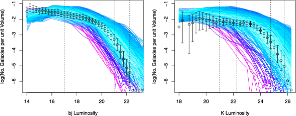
Of all the outputs produced by Galform, we focus our analysis on by far the most important: the bj and K luminosity functions, which give the log number of blue or red (i.e., young or old) galaxies, respectively, per unit volume, binned by luminosity (Norberg et al. (2002)). These observed luminosity functions, shown as the black points in Figure 2, are considered to be the benchmark by which models of galaxy formation are judged. Models will be discarded if they do not match these luminosity functions alone, and determining the set of input parameters that give rise to such matches is of inherent scientific worth, as it will be highly informative regarding the various physical processes involved in galaxy formation. Determining if any matches even exist and, if so, obtaining a large set of runs that match this data for use in future analysis are major goals of the project.

3 Bayesian History Matching

This study concerns Bayesian history matching, to identify a collection of input parameter choices for Galform which give acceptable matches to certain measurements on the universe. History matching is a common term in the oil industry, where it is used to describe the adjustment of a model of a reservoir, by modifying the input parameter choices, until it closely reproduces the historical production and pressure profiles recorded in that reservoir. In Durham, we have developed a general Bayesian approach to this problem for oil reservoirs, expanding the use of the term from finding a single match to searching for all such matches. A good description of this work can be found in Craig et al. (1997). This history matching methodology is part of the general Bayesian treatment of uncertainty in physical systems modelled by complex computer simulators. A good reference for this area is the website for the Managing Uncertainty in Complex Models (MUCM) project, http://www.mucm.ac.uk. Here, we focus on those aspects of the general methodology that are most relevant to history matching.

We want to use the Galform simulator to reproduce the observed history of the physical system. Therefore, we need to consider how good the match should be in order to be acceptable. We must recognise the limitations of the simulator as a representation of the physical system. Our models approximate and simplify both the properties of the system and the physical principles used to generate the corresponding system behaviour. Even so, the mathematical implementation is still too complex for precise solution, and so is further simplified and approximated. Add to this our uncertainty about initial conditions, boundary conditions and forcing functions for the system, and it is clear that we must assess the structural discrepancy between model outcomes, even if well chosen, and actual physical behaviour of the system. Our judgements about structural discrepancy determine our views about the quality of the match that we may achieve.

The general structure of the problem is as follows. We represent the simulator as a vector function, taking inputs $x$ which represent system properties, and returning outputs $f(x)$ which are intended to correspond to certain properties, $y$, of the physical system. We have observations $z$ on $y$. We represent the difference between $z$ and $y$ by the relation

$$z=y+e,$$ (1)

where $e$ is the vector of random observational errors, taken to be independent of $y$ and, typically, of each other. If $f(x)$ was a perfect representation of the system, then we would only accept a choice $x^{*}$ as representing the system if $f(x^{*})=y$. Because we can only compare $f(x^{*})$ with $z$, we would therefore require the match between $f(x^{*})$ and $z$ to be probabilistically consistent with the relation $z=f(x^{*})+e$.

However, because of structural discrepancy, even if we had evaluated an appropriate choice $f(x^{*})$, we would still be uncertain about the true system value, $y$. If we represent this residual uncertainty by the random structural discrepancy vector $\varepsilon$ and consider $\varepsilon$ to be independent of $f(x^{*})$, then we can write

$$y=f\bigl{(}x^{*}\bigr{)}+\varepsilon,$$ (2)

where, for example, the variance of each element of $\varepsilon$ expresses our judgement about how well the corresponding element of $f(x^{*})$ is expected to reproduce that element of the system, and the correlation between two elements of $\varepsilon$ expresses our judgements about the similarities of the issues relating to each component of the discrepancy. We may view $\varepsilon$ as a way of expressing the sense that we are prepared to tolerate a less than perfect match, and explore the effect of different choices for this tolerance on the space of acceptable parameter matches. [For a much more detailed treatment of the concept of model discrepancy, see Goldstein and Rougier (2009) and the accompanying discussion.] Specification of beliefs for $\varepsilon$ may partly be carried out by experiments on the simulator itself [e.g., by exploring the effect of perturbing the forcing function or adding some internal randomness to the propagation of an internal state vector propagated over time by the model; see, e.g., Goldstein, Seheult and Vernon (2013)]. However, a large component of such specification comes from the scientifically grounded but subjective judgements of the expert.

Combining (1) and (2), we therefore consider the match acceptable if it is probabilistically consistent with the relation

$$z=f\bigl{(}x^{*}\bigr{)}+\varepsilon+e.$$ (3)

Our aim is to identify the collection, $\chi(z)$, of all choices of $x^{*}$ which would give acceptable fits to historical data or, at the least, to identify a wide range of elements of $\chi(z)$. If our input parameter space is low dimensional, and the function is very fast to evaluate, then we can find $\chi(z)$ by evaluating the function everywhere and identifying the collection of all choices $x^{*}$ consistent with (3). However, for most complex physical models, it is infeasible to evaluate the simulator at enough choices to search the input space exhaustively. Therefore, we must construct a representation of our uncertainty about the value of the simulator at each input choice for which we have not yet evaluated the simulator. This representation is termed an emulator. The emulator both suggests an approximation to the function and also contains an assessment of the likely magnitude of the error of the approximation. A common choice of form for emulation of component $f_{i}$ is

$$f_{i}(x)=\sum_{j}\beta_{ij}g_{ij}(x_{A_{i}})+u_{i}(x_{A_{i}})+w_{i}(x),$$ (4)

where the active variables $x_{A_{i}}$ are subsets of the 17 inputs, $B=\{\beta_{ij}\}$ are unknown scalars, $g_{ij}$ are known deterministic functions of $x_{A_{i}}$, for example, polynomials, $u_{i}(x_{A_{i}})$ is a Gaussian process or, in a less fully specified version, a weakly second order stationary stochastic process, with, for example, correlation function

$$\operatorname{Corr}\bigl{(}u_{i}(x_{A_{i}}),u_{i}\bigl{(}x^{\prime}_{A_{i}}\bigr{)}\bigr{)}$$

(5)

$$\quad=\exp\bigl{(}-\bigl{\|}x_{A_{i}}-x_{A_{i}}^{\prime}\bigr{\|}^{2}/\theta_{i}^{2}\bigr{)},$$

and $w_{i}(x)$ is an uncorrelated nugget. $Bg(x)$ expresses global variation in $f$, while $u(x)$ expresses local variation in $f$. We fit the emulators, given a collection of carefully chosen simulator evaluations, using our favourite statistical tools, guided by expert judgement. We use detailed diagnostics to check emulator validity. A good introduction to function emulation is given by O’Hagan (2006).

Using the emulator, we can obtain, for each choice of inputs $x$, the mean and variance, $\mathrm{E}(f(x))$ and $\operatorname{Var}(f(x))$. Applying relation (3), for $x\in\chi(z)$, gives $\operatorname{Var}(z_{i}-\mathrm{E}(f_{i}(x)))=\operatorname{Var}(f_{i}(x))+\operatorname{Var}(\varepsilon_{i})+\operatorname{Var}(e_{i})$. We can therefore calculate, for each output $f_{i}(x)$, the “implausibility” if we consider the value $x$ to be a member of $\chi(z)$. This is the standardised distance between $z_{i}$ and $\mathrm{E}(f_{i}(x))$, which is

$$I_{(i)}^{2}(x) = \bigl{|}z_{i}-\mathrm{E}\bigl{(}f_{i}(x)\bigr{)}\bigr{|}^{2}$$

$${}/\bigl{[}\operatorname{Var}\bigl{(}f_{i}(x)\bigr{)}+\operatorname{Var}(\varepsilon_{i})+\operatorname{Var}(e_{i})\bigr{]}.$$

Large values of $I_{(i)}(x)$ suggest that it is implausible that $x\in\chi(z)$. The implausibility calculation can be performed univariately, or by multivariate calculation over sub-vectors. The implausibilities are then combined, such as by using $I_{M}(x)=\max_{i}I_{(i)}(x)$, and can then be used to identify regions of $x$ with large $I_{M}(x)$ as implausible. With this information, we can then refocus our analysis on the “nonimplausible” regions of the input space, by making more simulator runs and refitting our emulator over such subregions and iteratively repeating the analysis. This is a form of iterative global search aimed at finding all choices of $x$ which would give acceptable fits to historical data. We may find $\chi(z)$ is empty, which is a strong warning of problems with our simulator or with our data.

History matching may be compared with model calibration which aims to identify the one “true” value of the input parameters $x^{*}$. Often, we will prefer to carry out a history match because either we do not believe in a unique true input value for the model or we are unsure as to whether any good choices of input parameters exist. Further, full probabilistic calibration analysis may be difficult, as, typically, $\chi(z)$ will comprise a tiny volume of the original parameter space. Therefore, even if there is an eventual intention to carry out a full probabilistic calibration, it is often good practice to history match first, in order to check the simulator and to reduce the original parameter space down to $\chi(z)$.

Finally, a note on the methods used in this study. We may carry out a full Bayes analysis, with complete joint probabilistic specification of all of the uncertain quantities in the problem. Alternatively, we may carry out a Bayes linear analysis, based just on a prior specification of the means, variances and covariances of all quantities of interest. Probability is the most common choice, but there are advantages in working with expectations, as the uncertainty specification is simpler and the analysis is much more technically straightforward. Bayes linear analysis [for a detailed account, see Goldstein and Wooff (2007)] is based around these updating equations for mean and variance:

$$\mathsf{E}_{z}[y] = \mathrm{E}(y)+\operatorname{Cov}(y,z)\operatorname{Var}(z)^{-1}\bigl{(}z-\mathrm{E}(z)\bigr{)},$$ (7)

$$\qquad\mathsf{Var}_{z}[y] = \operatorname{Var}(y)$$

$${}-\operatorname{Cov}(y,z)\operatorname{Var}(z)^{-1}\operatorname{Cov}(z,y).$$

History matching fits naturally with this approach and the Galform study has been analysed using Bayes linear methods. There are natural probabilistic counterparts, which we expect could have found similar history matches to those we discovered, but with considerably more effort in prior specification and computation.

Figure 3: Left panel: the sd of each contribution from the various sources of uncertainty for the full range of the bj luminosity function (the $x$-axis is the same as Figure 2). The vertical lines represent the three bj outputs chosen for emulation in wave 1. Green line: the total uncertainty due to all contributions; this value is used for the error bars in Figure 2. The K luminosity results are similar. The residual standard deviation $\sigma$ for waves 1 to 3 (top right panel) and the adjusted R² for waves 1 to 3 (bottom right panel) for the polynomial part $\mathit{Bg}(x)$ of each emulator [equation (4)]. We fit high-dimensional cubic polynomials due to having large run numbers. First 6 connected points: bj outputs chosen for emulation, later 5 are the K outputs (shown as vertical lines in Figure 6, left and right panels, resp.). See Vernon, Goldstein and Bower (2010).

4 Application to a Galaxy Formation Simulation

4.1 Sources of Uncertainty

We now describe the application of the methodology introduced in Section 3 to the Galform model described in Section 2. In order to determine the meaning of an acceptable match, it is essential that we identify all sources of uncertainty that lie between the model output $f(x)$ and reality $y$. Note that the majority of these uncertainties have been neglected or ignored in even the most detailed of previous analyses. As discussed in Section 3, the uncertainties separate into two classes: the model discrepancy $\varepsilon$ and the observation errors $e$. In the case of Galform, the model discrepancy was decomposed into three uncorrelated contributions $\varepsilon=\Phi_{\mathrm{IA}}+\Phi_{\mathrm{DM}}+\Phi_{E}$ where:

$\Phi_{\mathrm{IA}}$ Inactive variable uncertainty: due to coding issues, for the first three waves we could not vary all 17 parameters simultaneously. The 9 least active inputs were fixed and their effects represented by this term.

$\Phi_{\mathrm{DM}}$ dark matter uncertainty: unknown configuration of dark matter in the universe, assessed from computer model experiments on the 40 sub-volumes.

Table 2: Summary of the 4 waves of emulation. Col. 2: the no. of model runs used to construct the emulator; col. 3: no. of outputs emulated, col. 4: the no. of active variables; col. 5–8: the implausibility thresholds; col. 9: the percentage of the parameter space deemed nonimplausible

Wave	Runs	Outputs emul.	Active inputs	$\bolds{I_{M}}$	$\bolds{I_{2M}}$	$\bolds{I_{3M}}$	$\bolds{I_{\mathit{MV}}}$	% Space
1	0993	17	15	–	2.7	2.3	–	14.9%
2	1414	11	18	–	2.7	2.3	–	5.9%
3	1620	11	18	–	2.7	2.3	26.75	1.6%
4	2011	11	10	3.2	2.7	2.3	26.75	0.26%
5	2000	–	–	2.5	–	–	26.75	0.039%

$\Phi_{E}$ Subjective expert assessment of model discrepancy between full Galform model (all 17 inputs and correct dark matter) and real universe. Using a detailed elicitation tool, the cosmologist was able to specify a multivariate covariance structure for $\Phi_{E}$ representing beliefs about the known deficiencies of the model (over/under abundance of matter and ageing rates of red/blue galaxies), leading to positive correlations between the discrepancy for bj outputs and smaller positive correlations across bj and K outputs. Our methods also incorporate a sensitivity analysis regarding the expert’s assessment of $\Phi_{E}$ (Goldstein and Vernon (2009)).

The four contributions to the observation errors $e$ are as follows:

Luminosity zero point error: correlated uncertainty across luminosity outputs due to difficulty of defining galaxy of “zero” brightness.

The $k+e$ error: a highly correlated error on all output points due to (i) galaxies being so far away it takes light billions of years to reach us and (ii) galaxies moving away from us so quickly their light is redshifted.

Normalisation error: correction for over/under population of galaxies in local universe using theoretical considerations of universe on large scales.

Galaxy production error: uncertain theoretical correction due to bright/faint galaxies being measured up to relatively large/short distances from Earth.

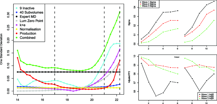
Note that the observations represent theory laden data having been heavily preprocessed prior to our analysis and, hence, it would be dangerous to neglect any one of the above observational errors. All the above uncertainties are shown for the full bj luminosity function in Figure 3 (left panel), plotted as one standard deviation against luminosity [the $x$-axis is the same as Figure 2 (left panel)].

Figure 4: The top three panels give waves 1, 2 and 3 minimised implausibility projection plots in the $V_{\mathrm{hot},\mathrm{disk}}$–${\alpha_{\mathrm{cool}}}$ plane, representing $I_{2M}(x)$ minimised across the remaining 15 inputs. The red region indicates high implausibility where input points will be discarded, green/yellow: nonimplausible points. The bottom three panels give the optical depth plots, showing the fraction of the hidden 15-dimensional volume that satisfies the implausibility cutoff, at that grid-point.

4.2 Emulation and Iterative History Matching

We proceed to emulate in iterations or waves as described in Section 3. In each wave we design a space filling set of runs, choose a subset of viable outputs $f_{i}(x)$ for emulation, for each output choose a subset of active inputs $x_{A}$ and then construct a Bayes linear emulator for $f_{i}(x)$ using equations (4) and (3). The emulators are combined with the subjectively assessed model discrepancy and the observation errors to produce an implausibility measure $I_{(i)}(x)$ for each output [equation (3)]. We then discard regions of input space $x$ that do not satisfy cutoffs on $I_{M}(x)$, $I_{2M}(x)$ and $I_{3M}(x)$ [the first, second and third highest $I_{(i)}(x)$]. Table 2 summarises the 4 waves that were performed. For example, in wave 1 we emulated only 7 outputs (shown as vertical dotted lines in Figure 2) and used only 5 active variables for each emulator, imposing cautious implausibility constraints on only $I_{2M}(x)$ and $I_{3M}(x)$ [as $I_{M}(x)$ can be sensitive to inaccuracies in the emulators]. At each wave we performed 200 diagnostic runs to check emulator performance.

Figure 5: Left: wave 4 minimised implausibility (below diagonal) and optical depth (above diagonal) projections (see Figure 4). Right: the wave 5 runs coloured by the implausibility consistent with the left panel, now with no emulator uncertainty, confirming the wave 4 predictions.

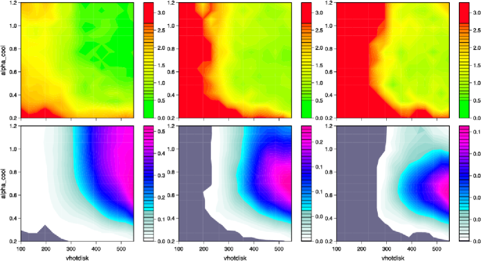
In each new wave we perform more runs, the emulators become more accurate, the implausibility measures more informative and, hence, we are able to discard more space as implausible than in the previous wave. Explicit improvement in the emulators over the first three waves is shown in Figure 3 (top right and bottom right panels). We expect this emulator improvement, as at each wave (a) there are a higher density of runs which improves the Gaussian process part of the emulator, (b) we can choose more active inputs $x_{A}$, (c) we are emulating a smoother function since it is defined over a smaller volume and (d) we can hence choose more outputs to emulate. The iterative nature of the space reduction process is the main reason the history matching approach is so powerful and is shown in Figure 4 for waves 1 to 3. The percentage of input space remaining is given in Table 2.

4.3 Iterative History Matching: Waves 4 and 5 Results

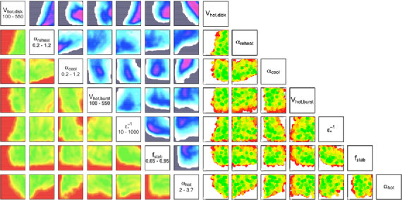
We performed 4 waves of history matching in order to identify the set of input parameters consistent with the luminosity function observations. Various 2D projections of the nonimplausible set of inputs at wave 4 are shown in Figure 5 (left panel), where the projections are onto the subspaces of pairs of 7 of the most interesting input parameters, out of the full 17 given in Table 1. These projections, along with higher-dimensional equivalents, provide the cosmologists with detailed insight into to the behaviour of the Galform model: indeed, there was much initial surprise as to the extent of the nonimplausible region in some directions, despite it occupying a tiny percentage of the original input space of only $0.039\%$.

Figure 6: Left: the bj luminosity function output for the first 500 runs of waves 1, 2 and 3 and the wave 5 acceptable runs that satisfy $I_{M}(x)<2.5$. Right: K luminosity. The disparity at luminosity $\leq$ 19 between K luminosity data and wave 5 runs is due to the limited resolution of the dark matter simulation [see Bower et al. (2006)] and so is not considered of interest.

As the wave 4 emulator variances were smaller than the combined model discrepancy and observation errors, the iterations were terminated. A final set of wave 5 runs was generated both to confirm the predictions made by the wave 4 emulator of the extent of the region of acceptable matches and to obtain a large set of acceptable runs for use by the cosmologists, a major goal of the project. These wave 5 runs are shown in Figure 5 (right panel) with the same implausibility colour scale as in the left panel, but now without any emulator uncertainty. Large numbers of acceptable runs were found, and 306 runs were found to satisfy the more strict cutoff $I_{M}(x)<2.5$, superior to any matches previously found by the cosmologists. The outputs of these acceptable runs, along with those of previous waves, are shown in Figure 6. Note that the acceptable runs are good matches across all luminosities, not just at the 11 ouptuts chosen for emulation.

5 Conclusion

The task of finding matches between complex galaxy formation simulation output and observations of the real universe represents a fundamental challenge within cosmology. Even to define what we mean by an acceptable match requires an assessment of model discrepancy, which can only come through a, necessarily subjective, scientific judgement based on many years of experience in constructing such simulations. Therefore, this problem fits naturally into a Bayesian framework, in which we treat all of the uncertainties arising from properties of the simulator or of the data in a unified manner.

The resulting problem, of identifying matches consistent with our uncertainty measures, is extremely challenging, involving understanding the simulator’s behaviour over a high-dimensional input parameter space. It is difficult to see how to proceed without the use of carefully constructed Bayesian emulators that represent our beliefs about the behaviour of the deterministic function at all points in the input space and which are fast to evaluate. These emulators are used within an iterative history matching strategy that seeks only to emulate in detail the most interesting parts of the input space, and thus provides a global search algorithm which gives a practical and tractable Bayesian solution to the problem.

We have demonstrated this solution for the galaxy formation simulator. Specifically, we have identified the regions of input space of interest, occupying $0.039\%$ of the initial volume, and provided the cosmologists with a large set of runs that yield acceptable matches: a major goal of the project. An account of the impact of this approach within cosmology is given in Bower et al. (2010). A history match is in most cases sufficient for the scientists’ needs, both for model analysis and development. However, even if a more detailed, fully probabilistic Bayesian analysis is required, perhaps of a well-tested and highly accurate model, a history match is usually a good precursor to the calibration exercise, to rule out the vast areas of input space that would possess extremely low posterior probability.

References

- Bower et al. (2006) {barticle}[author] \bauthor\bsnmBower, \bfnmR. G.\binitsR. G., \bauthor\bsnmBenson, \bfnmA. J.\binitsA. J. \betalet al. (\byear2006). \btitleThe broken hierarchy of galaxy formation. \bjournalMon. Not. Roy. Astron. Soc. \bvolume370 \bpages645–655. \bptokimsref \endbibitem
- Bower et al. (2012) {barticle}[author] \bauthor\bsnmBower, \bfnmR. G.\binitsR. G., \bauthor\bsnmBenson, \bfnmA. J.\binitsA. J. \betalet al. (\byear2012). \btitleWhat shapes the galaxy mass function? Exploring the roles of supernova-driven winds and AGN. \bjournalMon. Not. Roy. Astron. Soc. \bvolume422 \bpages2816. \bptokimsref \endbibitem
- Bower et al. (2010) {barticle}[author] \bauthor\bsnmBower, \bfnmR. G.\binitsR. G., \bauthor\bsnmVernon, \bfnmI.\binitsI., \bauthor\bsnmGoldstein, \bfnmM.\binitsM. \betalet al. (\byear2010). \btitleThe parameter space of galaxy formation. \bjournalMon. Not. Roy. Astron. Soc. \bvolume407 \bpages2017–2045. \bptokimsref \endbibitem
- Craig et al. (1997) {bincollection}[mr] \bauthor\bsnmCraig, \bfnmP. S.\binitsP. S., \bauthor\bsnmGoldstein, \bfnmM.\binitsM., \bauthor\bsnmSeheult, \bfnmA. H.\binitsA. H. and \bauthor\bsnmSmith, \bfnmJ. A.\binitsJ. A. (\byear1997). \btitlePressure matching for hydrocarbon reservoirs: A case study in the use of Bayes linear strategies for large computer experiments. In \bbooktitleCase Studies in Bayesian Statistics (\beditor\bfnmC.\binitsC. \bsnmGatsonis, \beditor\bfnmJ. S.\binitsJ. S. \bsnmHodges, \beditor\bfnmR. E.\binitsR. E. \bsnmKass, \beditor\bfnmR.\binitsR. \bsnmMcCulloch, \beditor\bfnmP.\binitsP. \bsnmRossi and \beditor\bfnmN. D.\binitsN. D. \bsnmSingpurwalla, eds.) \bvolume3 \bpages36–93. \bpublisherSpringer, \blocationNew York. \bptokimsref \endbibitem
- Goldstein and Rougier (2009) {barticle}[mr] \bauthor\bsnmGoldstein, \bfnmMichael\binitsM. and \bauthor\bsnmRougier, \bfnmJonathan\binitsJ. (\byear2009). \btitleReified Bayesian modelling and inference for physical systems (with discussion). \bjournalJ. Statist. Plann. Inference \bvolume139 \bpages1221–1239. \biddoi=10.1016/j.jspi.2008.07.019, issn=0378-3758, mr=2479863 \bptokimsref \endbibitem
- Goldstein, Seheult and Vernon (2013) {bincollection}[author] \bauthor\bsnmGoldstein, \bfnmM.\binitsM., \bauthor\bsnmSeheult, \bfnmA.\binitsA. and \bauthor\bsnmVernon, \bfnmI.\binitsI. (\byear2013). \btitleAssessing model adequacy. In \bbooktitleEnvironmental Modelling: Finding Simplicity in Complexity \bpublisherWiley, \blocationNew York. \bptokimsref \endbibitem
- Goldstein and Vernon (2009) {bincollection}[author] \bauthor\bsnmGoldstein, \bfnmM.\binitsM. and \bauthor\bsnmVernon, \bfnmI.\binitsI. (\byear2009). \btitleBayes linear analysis of imprecision in computer models, with application to understanding the Universe. In \bbooktitleISIPTA’09: Proceedings of the 6th International Symposium on Imprecise Probability: Theories and Applications \bpages441–450. \bpublisherSIPTA, \blocationLugano, Switzerland. \bptokimsref \endbibitem
- Goldstein and Wooff (2007) {bbook}[mr] \bauthor\bsnmGoldstein, \bfnmMichael\binitsM. and \bauthor\bsnmWooff, \bfnmDavid\binitsD. (\byear2007). \btitleBayes Linear Statistics: Theory and Methods. \bpublisherWiley, \blocationChichester. \biddoi=10.1002/9780470065662, mr=2335584 \bptokimsref \endbibitem
- Norberg et al. (2002) {barticle}[author] \bauthor\bsnmNorberg, \bfnmP.\binitsP., \bauthor\bsnmCole, \bfnmS.\binitsS. \betalet al. (\byear2002). \btitleThe 2dF galaxy redshift survey: The -band galaxy luminosity function and survey selection function. \bjournalMon. Not. Roy. Astron. Soc. \bvolume336 \bpages907–934. \bptokimsref \endbibitem
- O’Hagan (2006) {barticle}[author] \bauthor\bsnmO’Hagan, \bfnmA.\binitsA. (\byear2006). \btitleBayesian analysis of computer code outputs: A tutorial. \bjournalReliability Engineering and System Safety \bvolume91 \bpages1290–1300. \bptokimsref \endbibitem
- Vernon, Goldstein and Bower (2010) {barticle}[mr] \bauthor\bsnmVernon, \bfnmIan\binitsI., \bauthor\bsnmGoldstein, \bfnmMichael\binitsM. and \bauthor\bsnmBower, \bfnmRichard G.\binitsR. G. (\byear2010). \btitleGalaxy formation: A Bayesian uncertainty analysis (with discussion). \bjournalBayesian Anal. \bvolume5 \bpages619–669. \bidmr=2740148 \bptokimsref \endbibitem