Ubiquitous antinodal quasiparticles and deviation from simple d-wave form in underdoped Bi-2212: Supplementary materials

To assess the effects of instrument resolution on the measured gap function, we simulate spectra using a model spectral function proposed by Kordyuk et al. Kordyuk et al. (2003):

$$\Sigma"(\mathbf{k},\omega)=\sqrt{(\alpha\omega)^{2}+(\beta T)^{2}}$$ (1)

The simulations in Fig. S1 use the values $(\alpha,\beta,T)=(0.2,9.3,10K)$ which produces spectra comparable to experiments. An additional energy-independent momentum broadening of 0.006 $\AA^{-1}$ is included for better agreement with data. The band structure is taken to be a tight binding model with parameters

$$(\mu,t,t^{\prime},t^{\prime\prime},t^{\prime\prime\prime},t^{\prime\prime\prime\prime})=(0.091,-0.72,0.063,-0.17,-0.015,0.073)$$ (2)

The resolution function is taken to be a two-dimensional Gaussian in energy and momentum with values chosen to be relevant to experiments. Momentum resolution perpendicular to the analyzer slit is neglected.

Instrumental resolution not only broadens spectra, but it can also move the peak position of energy distribution curves (EDCs) slightly. Because there is no spectral weight above E_F in a low-temperature experiment, applying a convolution operation to a band which crosses E_F will tend to push weight asymmetrically near E_F. In the cuprates, the near-nodal region is most strongly affected by resolution effects because the Fermi velocity is larger. This is seen in Fig. S1(h)-(j) which shows symmetrized EDCs at k_F for three cuts indicated in panel (k). Closer to the node, instrumental energy resolution pushes the EDC peak to higher binding energy, but this effect is less pronounced at the antinode where bands are less dispersive.

The simulations are summarized in Fig. S1(a)-(d) which shows gaps around the Fermi surface for different choices of instrument resolution. The gap function is deliberately chosen to deviate from a simple d-wave form, and is instead described by a form with a higher harmonic: $\Delta(\theta)=\Delta_{0}*[\cos(2\theta)+(1-B)*\cos(6\theta)]$. The parameter B quantifies the degree of deviation from a simple d-wave form, with B$=$1 signifying a simple d-wave form and smaller values indicating greater deviation from a simple d-wave form. With increasing energy resolution and identical momentum resolution, the B parameter approaches 1, indicating decreasing deviation from a simple d-wave form. This may be one of the reasons Ref. Zhao et al., 2013 reports a simple d-wave form for all dopings. When the deviation from a simple d-wave form is subtle, poorer resolution can obscure this effect. Increasing the momentum resolution (Fig. S1(d)) can also smooth out subtle features in the gap function.

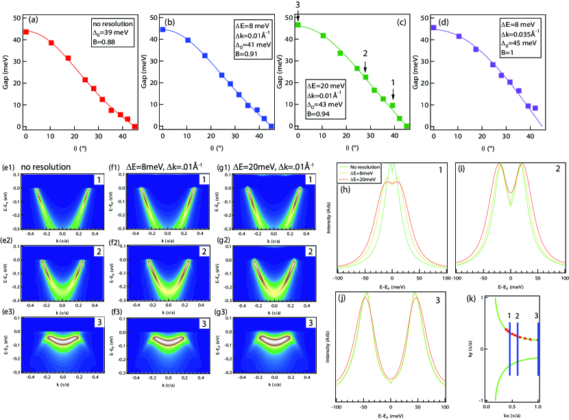
Figure S1: (a)-(d) Gap vs Fermi surface angle for various choices of energy and momentum resolution in simulation. Fits are to a d-wave gap with a higher harmonic term: $\Delta(\theta)=\Delta_{0}*[\cos(2\theta)+(1-B)*\cos(6\theta)]$. Panel (c) marks the three cuts which are detailed in subsequent panels. (e)-(g) simulated data with cuts taken parallel to the Brilliouin zone boundary. In (f)-(g), data has been convolved with a resolution function. (h)-(j) EDCs at k_F with varying resolution. (k) Fermi surface schematic, Fermi crossings used in (a)-(d), and cuts used in (e)-(g).

References

- Kordyuk et al. (2003) A. A. Kordyuk, S. V. Borisenko, M. Knupfer, and J. Fink, Phys. Rev. B 67, 064504 (2003).
- Zhao et al. (2013) J. Zhao, U. Chatterjee, D. Ai, D. Hinks, H. Zheng, G. Gu, S. Rosenkranz, J.-P. Castellan, H. Claus, M. R. Norman, M. Randeria, and J. C. Campuzano, Proc. Nat. Acad. Sci. 110, 17774 (2013).