Discrete Convexity and Polynomial Solvability
in Minimum 0-Extension Problems

Abstract

A $0$-extension of graph ${\mit\Gamma}$ is a metric $d$ on a set $V$ containing the vertex set $V_{{\mit\Gamma}}$ of ${\mit\Gamma}$ such that $d$ extends the shortest path metric of ${\mit\Gamma}$ and for all $x\in V$ there exists a vertex $s$ in ${\mit\Gamma}$ with $d(x,s)=0$. The minimum $0$-extension problem 0-Ext$[{\mit\Gamma}]$ on ${\mit\Gamma}$ is: given a set $V\supseteq V_{{\mit\Gamma}}$ and a nonnegative cost function $c$ defined on the set of all pairs of $V$, find a $0$-extension $d$ of ${\mit\Gamma}$ with $\sum_{xy}c(xy)d(x,y)$ minimum. The $0$-extension problem generalizes a number of basic combinatorial optimization problems, such as minimum $(s,t)$-cut problem and multiway cut problem.

Karzanov proved the polynomial solvability of 0-Ext$[{\mit\Gamma}]$ for a certain large class of modular graphs ${\mit\Gamma}$, and raised the question: What are the graphs ${\mit\Gamma}$ for which 0-Ext$[{\mit\Gamma}]$ can be solved in polynomial time? He also proved that 0-Ext$[{\mit\Gamma}]$ is NP-hard if ${\mit\Gamma}$ is not modular or not orientable (in a certain sense).

In this paper, we prove the converse: if ${\mit\Gamma}$ is orientable and modular, then 0-Ext$[{\mit\Gamma}]$ can be solved in polynomial time. This completes the classification of graphs ${\mit\Gamma}$ for which 0-Ext$[{\mit\Gamma}]$ is tractable. To prove our main result, we develop a theory of discrete convex functions on orientable modular graphs, analogous to discrete convex analysis by Murota, and utilize a recent result of Thapper and Živný on valued CSP.

1 Introduction

By a (semi)metric $d$ on a finite set $V$ we mean a nonnegative symmetric function on $V\times V$ satisfying $d(x,x)=0$ for all $x\in V$ and the triangle inequalities $d(x,y)+d(y,z)\geq d(x,z)$ for all $x,y,z\in V$. An extension of a metric space $(S,\mu)$ is a metric space $(V,d)$ with $V\supseteq S$ and $d(s,t)=\mu(s,t)$ for $s,t\in S$. An extension $(V,d)$ of $(S,\mu)$ is called a $0$-extension if for all $x\in V$ there exists $s\in S$ with $d(s,x)=0$.

Let ${\mit\Gamma}$ be a simple connected undirected graph with vertex set $V_{{\mit\Gamma}}$. Let $d_{\mit\Gamma}$ denote the shortest path metric on $V_{\mit\Gamma}$ with respect to the uniform unit edge-length of ${\mit\Gamma}$. The minimum $0$-extension problem 0-Ext$[{\mit\Gamma}]$ on ${\mit\Gamma}$ is formulated as:

0-Ext${[{\mit\Gamma}]}$: 

Given $V\supseteq V_{{\mit\Gamma}}$ and $\displaystyle c:{V\choose 2}\to{\bf Q}_{+}$,

                 

minimize $\displaystyle\sum_{xy\in{V\choose 2}}c(xy)d(x,y)$ over all $0$-extensions $(V,d)$ of $(V_{{\mit\Gamma}},d_{{\mit\Gamma}})$.

Here ${V\choose 2}$ denotes the set of all pairs of $V$. The minimum $0$-extension problem is formulated by Karzanov [32], and is equivalent to the following classical facility location problem, known as multifacility location problem [55], where we let $V\setminus V_{{\mit\Gamma}}:=\{1,2,\ldots,n\}$:

(1.1) Min. $$\sum_{s\in V_{{\mit\Gamma}}}\sum_{1\leq j\leq n}c(sj)d_{{\mit\Gamma}}(s,\rho_{j})+\sum_{1\leq i<j\leq n}c(ij)d_{{\mit\Gamma}}(\rho_{i},\rho_{j})$$

s.t. $$\rho=(\rho_{1},\rho_{2},\ldots,\rho_{n})\in V_{{\mit\Gamma}}\times V_{{\mit\Gamma}}\times\cdots\times V_{{\mit\Gamma}}.$$

This problem can be interpreted as follows: We are going to locate $n$ new facilities $1,2,\ldots,n$ on graph ${\mit\Gamma}$, where the facilities communicate each other and communicate existing facilities on ${\mit\Gamma}$. The cost of the communication is propositional to the distance. Our goal is to find a location of minimum total communication cost. This classic facility location problem arises in many practical situations such as the image segmentation in computer vision, and related clustering problems in machine learning; see [36]. Also 0-Ext$[{\mit\Gamma}]$ includes a number of basic combinatorial optimization problems. For example, take as ${\mit\Gamma}$ the graph $K_{2}$ consisting of a single edge $st$. Then 0-Ext$[K_{2}]$ is the minimum $(s,t)$-cut problem. More generally, 0-Ext$[K_{m}]$ is the multiway cut problem on $m$ terminals. Therefore 0-Ext$[K_{m}]$ is solvable in polynomial time if $m=2$ and is NP-hard if $m>2$ [14].

This paper addresses the following problem considered by Karzanov [32, 34, 35].

What are the graphs ${\mit\Gamma}$ for which 0-Ext$[{\mit\Gamma}]$ is solvable in polynomial time?

Here such a graph is simply called tractable.

A classical result in location theory in the 1970’s is:

Theorem 1.1 ([51]; also see [37]).

If ${\mit\Gamma}$ is a tree, then 0-Ext$[{\mit\Gamma}]$ is solvable in polynomial time.

The tractability of graphs ${\mit\Gamma}$ is preserved under taking Cartesian products. Therefore, cubes, grid graphs, and the Cartesian product of trees are tractable. Chepoi [12] extended this classical result to median graphs as follows.

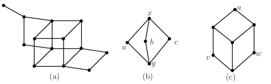
Figure 1: (a) a median graph, (b) $a,b,c$ have two medians $x,y$, and (c) $u,v,w$ have no median

A median of a triple $p_{1},p_{2},p_{3}$ of vertices is a vertex $m$ satisfying $d_{{\mit\Gamma}}(p_{i},p_{j})=d_{{\mit\Gamma}}(p_{i},m)+d_{{\mit\Gamma}}(m,p_{j})$ for $1\leq i<j\leq 3$. A median graph is a graph in which every triple of vertices has a unique median. Trees and their products are median graphs. See Figure 1 for illustration of the median concept.

Theorem 1.2 ([12]).

If ${\mit\Gamma}$ is a median graph, then 0-Ext$[{\mit\Gamma}]$ is solvable in polynomial time.

Karzanov [32] introduced the following LP-relaxation of 0-Ext$[{\mit\Gamma}]$.

Ext${[{\mit\Gamma}]}$: 

Given $V\supseteq V_{{\mit\Gamma}}$ and $c:\displaystyle{V\choose 2}\to{\bf Q}_{+}$,

                 

minimize $\displaystyle\sum_{xy\in{V\choose 2}}c(xy)d(x,y)$ over all extensions $(V,d)$ of $(V_{{\mit\Gamma}},d_{{\mit\Gamma}})$.

This relaxation Ext$[{\mit\Gamma}]$ is a linear program with size polynomial in the input size. Therefore, if for every input $(V,c)$, Ext$[{\mit\Gamma}]$ has an optimal solution that is a $0$-extension, then 0-Ext$[{\mit\Gamma}]$ is solvable in polynomial time. In this case we say that Ext$[{\mit\Gamma}]$ is exact. In the same paper, Karzanov gave a combinatorial characterization of graphs ${\mit\Gamma}$ for which Ext$[{\mit\Gamma}]$ is exact. A graph ${\mit\Gamma}$ is called a frame if
$(1.2)$ (1) ${\mit\Gamma}$ is bipartite, (2) ${\mit\Gamma}$ has no isometric cycle of length greater than $4$, and (3) ${\mit\Gamma}$ has an orientation $o$ with the property that for every 4-cycle $uv,vv^{\prime},v^{\prime}u^{\prime},u^{\prime}u$, one has $u\swarrow_{o}v$ if and only if $u^{\prime}\swarrow_{o}v^{\prime}$.
Here an isometric cycle in ${\mit\Gamma}$ means a cycle $C$ such that every pair of vertices in $C$ has a shortest path for ${\mit\Gamma}$ in this cycle $C$, and $p\swarrow_{o}q$ means that edge $pq$ is oriented from $q$ to $p$ by $o$.

Theorem 1.3 ([32]).

Ext$[{\mit\Gamma}]$ is exact if and only if ${\mit\Gamma}$ is a frame.

Theorem 1.4 ([32]).

If ${\mit\Gamma}$ is a frame, then 0-Ext$[{\mit\Gamma}]$ is solvable in polynomial time.

It is noted that the class of frames is not closed under taking Cartesian products, whereas the tractability of graphs is preserved under taking Cartesian products. Also it should be noted that Ext$[{\mit\Gamma}]$ is the LP-dual to the $d_{{\mit\Gamma}}$-weighted maximum multiflow problem, and 0-Ext$[{\mit\Gamma}]$ describes a combinatorial dual problem [32, 33]; see also [21, 22, 24, 23] for further elaboration of this duality.

Karzanov [32] also proved the following hardness result. For an undirected graph ${\mit\Gamma}$, an orientation with the property ((3)) (3) is said to be admissible. ${\mit\Gamma}$ is said to be orientable if it has an admissible orientation. ${\mit\Gamma}$ is said to be modular if every triple of vertices has a (not necessarily unique) median.

Theorem 1.5 ([32]).

If ${\mit\Gamma}$ is not orientable or not modular, then 0-Ext$[{\mit\Gamma}]$ is NP-hard.

In fact, a frame is precisely an orientable modular graph with the hereditary property that every isometric subgraph is modular; see [2]. A median graph is an orientable modular graph but the converse is not true. Moreover, a median graph is not necessarily a frame, and a frame is not necessarily a median graph. In [34], Karzanov proved a tractability theorem extending Theorem 1.2. He conjectured that 0-Ext$[{\mit\Gamma}]$ is tractable for a certain proper subclass of orientable modular graphs including frames and median graphs. He also conjectured that 0-Ext$[{\mit\Gamma}]$ is NP-hard for any graph ${\mit\Gamma}$ not in this class.

The main result of this paper is the tractability theorem for all orientable modular graphs. Thus the class of tractable graphs is larger than his expectation.

Theorem 1.6.

If ${\mit\Gamma}$ is orientable modular, then 0-Ext$[{\mit\Gamma}]$ is solvable in polynomial time.

Combining this result with Theorem 1.5, we obtain a complete classification of the graphs ${\mit\Gamma}$ for which 0-Ext$[{\mit\Gamma}]$ is solvable in polynomial time.

Overview.

In proving Theorem 1.6, we employ an axiomatic approach to optimization in orientable modular graphs. This approach is inspired by the theory of discrete convex analysis developed by Murota and his collaborators (including Fujishige, Shioura, and Tamura); see [17, 45, 48, 49, 47] and also [16, Chapter VII]. Discrete convex analysis is a theory of convex functions on integer lattice ${\bf Z}^{n}$, with the goal of providing a unified framework for polynomially solvable combinatorial optimization problems including network flows, matroids, and submodular functions. The theory that we are going to develop here is, in a sense, a theory of discrete convex functions on orientable modular graphs, with the goal of providing a unified framework for polynomially solvable 0-extension problems and related multiflow problems. We believe that our theory establishes a new link between previously unrelated fields, broadens the scope of discrete convex analysis, and opens a new perspective and new research directions.

Let us start with a simple observation to illustrate our basic idea. Consider a path $P_{m}$ of length $m$, and consider 0-Ext$[P_{m}]$, where $P_{m}$ is trivially an orientable modular graph. Then 0-Ext$[P_{m}]$ for input $V,c$ can be regarded as an optimization problem on the integer lattice ${\bf Z}^{n}$ as follows. Suppose that $V_{P_{m}}=\{1,2,3,\ldots,m\}$, and $s$ and $s+1$ are adjacent for $s=1,2,\ldots,m-1$. Then $d_{P_{m}}(s,t)=|s-t|$, and 0-Ext$[P_{m}]$ is equivalent to the minimization of the function

(1.3) $$\sum_{1\leq s\leq m}\sum_{1<j<n}c(sj)|s-\rho_{j}|+\sum_{1\leq i<j\leq n}c(ij)|\rho_{i}-\rho_{j}|$$

over all $(\rho_{1},\rho_{2},\ldots,\rho_{n})\in[0,m]^{n}\cap{\bf Z}^{n}$. This function is a simple instance of L^♮-convex functions, one of the fundamental classes of discrete convex functions. We do not give a formal definition of L^♮-convex functions here. The only important facts for us are the following properties of L^♮-convex functions in optimization:

• Local optimality implies global optimality.

• The local optimality can be checked by submodular function minimization.

• An efficient descent algorithm can be designed based on successive application of submodular function minimization.

As is well-known, submodular functions can be minimized in polynomial time [20, 30, 54]. Actually the function (1.3) can be minimized by successive application of minimum-cut computation [37, 51], a special case of submodular function minimization.

Motivated by this observation, we regard 0-Ext$[{\mit\Gamma}]$ as a minimization of a function defined on the vertex set of a product of ${\mit\Gamma}$, which is also orientable modular. We will introduce a class of functions, called L-convex functions, on an orientable modular graph. We show that our L-convex function satisfies analogues of (a), (b) and (c) above, and also that a multifacility location function, the objective function of 0-Ext$[{\mit\Gamma}]$, is an L-convex function, in our sense, on the product of ${\mit\Gamma}$. Theorem 1.6 is a consequence of these properties.

Let us briefly mention how to define L-convex functions, which constitutes the main body of this paper. Our definition is based on the Lovász extension [44], a well-known concept in submodular function theory [16], and a kind of construction of polyhedral complexes, due to Karzanov [32] and Chepoi [13], from a class of modular graphs. Let ${\mit\Gamma}$ be an orientable modular graph with admissible orientation $o$. We call a pair $({\mit\Gamma},o)$ a modular complex. It turns out that $({\mit\Gamma},o)$ can be viewed as a structure glued together from modular lattices, and gives rise to a simplicial complex as follows. Consider a cube subgraph $B$ of ${\mit\Gamma}$. The digraph $\vec{B}$ oriented by $o$ coincides with the Hasse diagram of a Boolean lattice. Consider the simplicial complex ${\mit\Delta}({\mit\Gamma},o)$ whose simplices are sets of vertices forming a chain of the Boolean lattice corresponding to some cube subgraph of ${\mit\Gamma}$; see Figure 2.

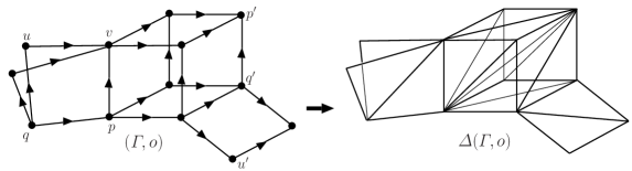
Figure 2: A construction of ${\mit\Delta}({\mit\Gamma},o)$

Each (abstract) simplex is naturally regarded as a simplex in the Euclidean space. ${\mit\Delta}({\mit\Gamma},o)$ is naturally regarded as a metrized simplicial complex. Then any function $g:V_{{\mit\Gamma}}\to{\bf R}$ is extended to $\overline{g}:{\mit\Delta}({\mit\Gamma},o)\to{\bf R}$ by interpolating $g$ on each simplex linearly; this is an analogue of the Lovász extension. The simplicial complex ${\mit\Delta}({\mit\Gamma},o)$ enables us to consider the neighborhood ${\cal L}_{p}^{*}$ around each vertex $p\in V_{{\mit\Gamma}}$, as well as the local behavior of $\overline{g}$ in ${\cal L}_{p}^{*}$.

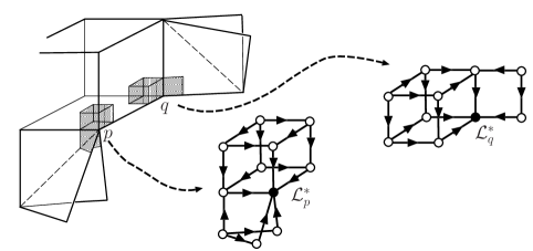
Figure 3: Neighborhood semilattices

As in Figure 3, neighborhood ${\cal L}^{*}_{p}$ can be described as a partially ordered set with the unique minimal element $p$. Then, by restricting $\overline{g}$ to ${\cal L}^{*}_{p}$, we obtain a function on ${\cal L}^{*}_{p}$ associated with each vertex $p$. In fact, the poset ${\cal L}^{*}_{p}$ is a modular semilattice, a semilattice analogue of a modular lattice introduced by Bandelt, van de Vel, and Verheul [5]. We first define submodular functions on modular semilattices, and next define L-convex functions on modular complex $({\mit\Gamma},o)$ as functions $g$ on $V_{{\mit\Gamma}}$ such that $\overline{g}$ is submodular on neighborhood semilattice ${\cal L}^{*}_{p}$ for each vertex $p$.

Then the multifacility location function, the objective of 0-Ext$[{\mit\Gamma}]$ (see (1.1)), is indeed an L-convex function on the $n$-fold product of ${\mit\Gamma}$, and the optimal solution of 0-Ext$[{\mit\Gamma}]$ can be obtained by successive application of submodular function minimization on the product of $n$ modular semilattices. Thus our problem reduces to the problem of minimizing submodular function $f$ on the product of modular semilattices ${\cal L}_{1},{\cal L}_{2},\ldots,{\cal L}_{n}$, where the input of the problem is ${\cal L}_{1},{\cal L}_{2},\ldots,{\cal L}_{n}$, and an evaluating oracle of $f$. We do not know whether this problem in general is tractable in the oracle model, but the submodular functions arising from 0-Ext$[{\mit\Gamma}]$ take a special form; they are the sum of submodular functions with arity $2$. Here the arity of a function $f$ is the number of variables of $f$. Namely, if a function $f$ on ${\cal L}={\cal L}_{1}\times{\cal L}_{2}\times\cdots\times{\cal L}_{n}$ is represented as

$$f(x)=h(x_{i_{1}},x_{i_{2}},\ldots,x_{i_{k}})\quad(x=(x_{1},x_{2},\ldots,x_{n})\in{\cal L})$$

for some function $h$ on ${\cal L}_{i_{1}}\times{\cal L}_{i_{2}}\times\cdots\times{\cal L}_{i_{k}}$ with $i_{1}<i_{2}<\cdots<i_{k}$, then the arity of $f$ is (at most) $k$. See (1.1); our objective function is a weighted sum of distance functions, which have arity $2$. This type of optimization problem with bounded arity is well-studied in the literature of valued CSP (valued constraint satisfaction problem) [7, 42, 53, 59]. Valued CSP deals with minimization of a sum of functions $f_{i}$ $(i=1,2,\ldots,m)$, where the arity $k_{i}$ of each $f_{i}$ is a part of the input; namely the input consists of all values of all functions $f_{i}$. Valued CSP admits an integer programming formulation, and its natural LP relaxation is called the basic LP-relaxation. Recently, Thapper and Živný [56] discovered a surprising criterion for the basic LP-relaxation of valued CSP to exactly solve the original valued CSP instance. They proved that if the class of valued CSP (the class of input objective functions) has a certain nice fractional polymorphism (a certain set of linear inequalities which any input function satisfies), then the basic LP-relaxation is exact. We prove that the class of submodular functions on modular semilattice admits such a fractional polymorphism. Then the sum of submodular functions with bounded arity can be minimized in polynomial time. Consequently we can solve 0-Ext$[{\mit\Gamma}]$ in polynomial time.

We believe that our classes of functions deserve to be called submodular and L-convex. Indeed, they include not only (ordinary) submodular/L-convex functions but also other submodular/L-convex-type functions. Examples are bisubmodular functions [9, 50, 52] (see [16, Section 3.5]), multimatroid rank functions by Bouchet [8], submodular functions on trees by Kolmogorov [38], $k$-submodular functions by Huber and Kolmogorov [27] (also see [18]), and skew-bisubmodular functions by Huber, Krokhin and Powell [29] (also see [19, 29, 28]). Moreover, combinatorial dual problems arising from a large class of (well-behaved) multicommodity flow problems, discussed in [21, 22, 24, 23, 31, 32, 33], fall into submodular/L-convex function minimization in our sense. This can be understood as a multiflow analogue of a fundamental fact in network flow theory: the minimum cut problem, the dual of maxflow problem, is a submodular function minimization. The detailed discussion on these topics will be given in a separate paper [26]; some of the results were announced by [25].

Organization.

In Section 2, we first explain basic notions of valued CSP and the Thapper-Živný criterion (Theorem 2.1) on the exactness of the basic LP relaxation. We then describe basic facts on modular graphs and modular lattices. In Section 3, we develop a theory of submodular functions on modular semilattices. We show that our submodular function satisfies the Thapper-Živný criterion, and that a sum of submodular functions with bounded arity can be minimized in polynomial time. In Section 4, we first explore several structural properties of orientable modular graphs. Based on the above mentioned idea, we define L-convex functions, and prove that our L-convex functions indeed have properties analogous to (a), (b) and (c) above. In Section 5, we formulate 0-Ext$[{\mit\Gamma}]$ as an optimization problem on a modular complex. We show that a multifacility location function, the objective function of 0-Ext$[{\mit\Gamma}]$, is indeed an L-convex function, and we prove Theorem 1.6. Our framework is applicable to a certain weighted version of 0-Ext$[{\mit\Gamma}]$. As a corollary, we give a generalization of Theorem 1.6 to general metrics, which completes classification of metrics $\mu$ for which the 0-extension problem on $\mu$ is polynomial time solvable (Theorem 5.9). In the last section (Section 6), we discuss a connection to a dichotomy theorem of finite-valued CSP obtained by Thapper and Živný [57] after the first submission of this paper. In fact, the complexity dichotomy (of form “either P or NP-hard”) of 0-Ext, established in this paper, can be viewed as a special case of their dichotomy theorem of finite-valued CSP.

Notation.

Let ${\bf Z},{\bf Q}$, and ${\bf R}$ denote the sets of integers, rationals, and reals, respectively. Let $\overline{{\bf R}}:={\bf R}\cup\{\infty\}$ and $\overline{{\bf Q}}:={\bf Q}\cup\{\infty\}$, where $\infty$ is an infinity element and is treated as: $\infty\cdot 0=0$, $x<\infty$ $(x\in{\bf R})$, $\infty+x=\infty$ $(x\in\overline{{\bf R}})$, $x\cdot\infty=\infty$ $(a\in{\bf R}:a>0)$. Let ${\bf Z}_{+},{\bf Q}_{+}$, and ${\bf R}_{+}$ denote the sets of nonnegative integers, nonnegative rationals, and nonnegative reals, respectively. For a function $f:X\to\overline{{\bf R}}$ on a set $X$, let $\mathop{\rm dom}f$ denote the set of elements $x\in X$ with $f(x)\neq\infty$.

For a graph ${\mit\Gamma}$, the vertex set and the edge set are denoted by $V_{{\mit\Gamma}}$ and $E_{{\mit\Gamma}}$, respectively. For a vertex subset $X$, ${\mit\Gamma}[X]$ denotes the subgraph of ${\mit\Gamma}$ induced by $X$. For a nonnegative edge-length $h:E_{{\mit\Gamma}}\to{\bf R}_{+}$, $d_{{\mit\Gamma},h}$ denotes the shortest path metric on $V_{{\mit\Gamma}}$ with respect to the edge-length $h$. When $h(e)=1$ for every edge $e$, $d_{{\mit\Gamma},h}$ is denoted by $d_{{\mit\Gamma}}$. A path is represented by a chain $(p_{1},p_{2},\ldots,p_{n})$ of vertices with $p_{i}p_{i+1}\in E_{{\mit\Gamma}}$. The Cartesian product ${\mit\Gamma}\times{\mit\Gamma}^{\prime}$ of graphs ${\mit\Gamma}$ and ${\mit\Gamma}^{\prime}$ is the graph with vertex set $V_{\mit\Gamma}\times V_{{\mit\Gamma}^{\prime}}$ and edge set given as: $(p,p^{\prime})$ and $(q,q^{\prime})$ are connected by an edge if and only if $p=q$ and $p^{\prime}q^{\prime}\in E_{{\mit\Gamma}^{\prime}}$ or $p^{\prime}=q^{\prime}$ and $pq\in E_{\mit\Gamma}$. The $n$-fold Cartesian product ${\mit\Gamma}\times{\mit\Gamma}\times\cdots\times{\mit\Gamma}$ of ${\mit\Gamma}$ is denoted by ${\mit\Gamma}^{n}$. In this paper, graphs and posets (partially ordered sets) are supposed to be finite.

2 Preliminaries

In this section, we give preliminary arguments for valued CSP, and modular graphs and modular (semi)lattices. Our references are [41, 59] for valued CSP and [3, 5, 6, 13, 58] for modular graphs and lattices. A further discussion on valued CSP is given in Section 6.

2.1 Valued CSP and fractional polymorphism

Let $D_{1},D_{2},\ldots,D_{n}$ be finite sets, and let $D:=D_{1}\times D_{2}\times\cdots\times D_{n}$. A constraint on $D$ is a function $f:D_{i_{1}}\times D_{i_{2}}\times\cdots\times D_{i_{k}}\to\overline{\bf R}$ for some $i_{1}<i_{2}<\cdots<i_{k}$, where $I_{f}:=\{i_{1},i_{2},\ldots,i_{k}\}$ is called the scope of $f$, and $k_{f}:=k$ is called the arity of $f$. Let $D_{I_{f}}:=D_{i_{1}}\times D_{i_{2}}\times\cdots\times D_{i_{f}}$, and for $x=(x_{1},x_{2},\ldots,x_{n})\in D$, let $x_{I_{f}}:=(x_{i_{1}},x_{i_{2}},\ldots,x_{i_{k}})\in D_{I_{f}}$. The valued CSP (valued constraint satisfaction problem) is:

VCSP:

Given a set ${\cal F}$ of constraints on $D$,

minimize $\displaystyle\sum_{f\in{\cal F}}f(x_{I_{f}})$ over all $x=(x_{1},x_{2},\ldots,x_{n})\in D$.

The input of VCSP is the set of all values of all constraints in ${\cal F}$, and hence its size is estimated by $O(|{\cal F}|N^{K}B)$, where $N:=\max_{1\leq i\leq n}|D_{i}|$, $K:=\max_{f\in{\cal F}}k_{f}$, and $B$ is the bit size to represent constraints in ${\cal F}$. By a constraint language we mean a (possibly infinite) set ${\mit\Lambda}$ of constraints. A constraint in ${\mit\Lambda}$ is called a ${\mit\Lambda}$-constraint. Let VCSP$[{\mit\Lambda}]$ denote the subclass of VCSP such that the input is restricted to a set of ${\mit\Lambda}$-constraints.

The minimum 0-extension problem 0-Ext$[{\mit\Gamma}]$ is formulated as an instance of VCSP. Let $D_{i}:=V_{{\mit\Gamma}}$ for $i=1,2,\ldots,n$. Define constraints $g_{i}:D_{i}\to{\bf R}$ and $f_{ij}:D_{i}\times D_{j}\to{\bf R}$ by

(2.1) $$g_{i}(\rho_{i}) := \sum_{s\in V_{{\mit\Gamma}}}c(si)d_{{\mit\Gamma}}(s,\rho_{i})\quad(\rho_{i}\in D_{i}),$$

$$f_{ij}(\rho_{i},\rho_{j}) := c(ij)d_{{\mit\Gamma}}(\rho_{i},\rho_{j})\quad((\rho_{i},\rho_{j})\in D_{i}\times D_{j}).$$

Define the input ${\cal F}$ of VCSP by

$${\cal F}:=\{g_{i}\mid 1\leq i\leq n\}\cup\{f_{ij}\mid 1\leq i<j\leq n\}.$$

Notice that the size of ${\cal F}$ is polynomial in $n$, ${\mit\Gamma}$, and the bit size representing $c$. Hence 0-Ext$[{\mit\Gamma}]$ is a particular subclass of VCSP.

VCSP admits the following integer programming formulation:

(2.2) Min. $$\sum_{f\in{\cal F}}\sum_{y\in\mathop{\rm dom}f}f(y)\lambda_{f,y}$$

s.t. $$\sum_{y\in\mathop{\rm dom}f:y_{i}=a}\lambda_{f,y}=\mu_{i,a}\quad(f\in{\cal F},i\in I_{f},a\in D_{i})$$

$$\sum_{a\in D_{i}}\mu_{i,a}=1\quad(1\leq i\leq n),$$

$$\lambda_{f,y}\in\{0,1\}\quad(f\in{\cal F},y\in\mathop{\rm dom}f),$$

$$\mu_{i,a}\in\{0,1\}\quad(1\leq i\leq n,a\in D_{i}).$$

Indeed, for each $i$ there uniquely exists $a_{i}\in D_{i}$ with $\mu_{i,a_{i}}=1$. Also for $f\in{\cal F}$ there uniquely exists $y\in\mathop{\rm dom}f$ such that $\lambda_{f,y}=1$ and $y_{i}=a_{i}$ for $i\in I_{f}$. Define $x=(x_{1},x_{2},\ldots,x_{n})$ by $x_{i}:=a_{i}$. Then $\lambda_{f,y}=1$ if and only if $x_{I_{f}}=y$. Therefore we obtain a solution $x=(x_{1},x_{2},\ldots,x_{n})$ of VCSP with the same objective value. Conversely, for a solution $x=(x_{1},x_{2},\ldots,x_{n})$ of VCSP, define $\mu_{i,a}:=1$ if $x_{i}=a$, and $\lambda_{f,y}:=1$ if $x_{I_{f}}=y$. The other variables are defined as zero. Then we obtain a solution of (2.2) with the same objective value.

Observe that there are $O(|{\cal F}|N^{K}+nN)$ variables and $O(|{\cal F}|KN+n)$ constraints. Therefore the size of this IP is bounded by a polynomial of the input size. The basic LP relaxation (BLP) is the linear problem obtained by relaxing the 0-1 constraints $\lambda_{f,y}\in\{0,1\}$ and $\mu_{i,a}\in\{0,1\}$ into $\lambda_{f,y}\geq 0$ and $\mu_{i,a}\geq 0$, respectively. In particular BLP can be solved in (strongly) polynomial time.

Recently Thapper and Živný [56] discovered a surprisingly powerful criterion for which BLP solves VCSP. To describe their result, let us introduce some notions. For a constraint language ${\mit\Lambda}$, BLP is said be exact for ${{\mit\Lambda}}$ if for every input ${\cal F}\subseteq{{\mit\Lambda}}$, the optimal value of BLP coincides with the optimal value of VCSP$[{\mit\Lambda}]$. An operation on $D_{i}$ is a function $D_{i}\times D_{i}\to D_{i}$. A (separable) operation $\vartheta$ on $D$ is a function $D\times D\to D$ such that $\vartheta$ is represented as

$$\vartheta(x,y)=(\vartheta_{1}(x_{1},y_{1}),\vartheta_{2}(x_{2},y_{2}),\ldots,\vartheta_{n}(x_{n},y_{n}))\quad(x,y\in D)$$

for some operations $\vartheta_{i}$ on $D_{i}$ for $i=1,2,\ldots,n$. A fractional operation $\omega$ is a function from the set of all operations to ${\bf R}_{+}$ such that the total sum $\sum\omega(\vartheta)$ over all operations $\vartheta$ is $1$. We denote a fractional operation $\omega$ by the form of a formal convex combination $\sum\omega(\vartheta)\vartheta$ of operations $\vartheta$. The support of $\omega$ is the set of operations $\vartheta$ with $\omega(\vartheta)>0$. For a constraint language ${\mit\Lambda}$, a fractional polymorphism is a fractional operation $\sum_{\vartheta}\omega({\vartheta})\vartheta$ on $D$ such that it satisfies

(2.3) $$\frac{f(x)+f(y)}{2}\geq\sum_{\vartheta}\omega(\vartheta)f(\vartheta(x,y))\quad(f\in{\mit\Lambda},x,y\in D_{I_{f}}),$$

where $\vartheta$ is regarded an operation on $D_{I_{f}}$ by $(\vartheta(x,y))_{i}:=\vartheta_{i}(x_{i},y_{i})$ for $i\in I_{f}$. For example, if $D_{i}$ is a lattice for each $i$, then $\frac{1}{2}\wedge+\frac{1}{2}\vee$ is nothing but a fractional polymorphism for submodular functions, i.e., functions $f$ satisfying $f(p)+f(q)\geq f(p\wedge q)+f(p\vee q)$ for $p,q\in D$.

Theorem 2.1 (Special case of [56, Theorem 5.1 ]).

If a constraint language ${\mit\Lambda}$ admits a fractional polymorphism $\omega$ such that the support of $\omega$ contains a semilattice operation, then BLP is exact for ${\mit\Lambda}$, and hence VCSP$[{\mit\Lambda}]$ can be solved in polynomial time.

Here a semilattice operation is an operation $\vartheta$ satisfying $\vartheta(a,a)=a$, $\vartheta(a,b)=\vartheta(b,a)$, and $\vartheta(\vartheta(a,b),c)=\vartheta(a,\vartheta(b,c))$ for $a,b,c\in D$. Although the feasible region of BLP is not necessarily an integral polytope, we can check whether there exists an optimal solution $x$ with $x_{i}=a\in D_{i}$ by comparing the optimal values of BLP for the input ${\cal F}$ and for ${\cal F}_{i,a}$, which is the set of cost functions obtained by fixing variable $x_{i}$ to $a$ for each cost function on ${\cal F}$. Necessarily BLP is exact for ${\cal F}_{i,a}$ if there is an optimal solution $x$ with $x_{i}=a$. Hence, after $n$ fixing procedures, we obtain an optimal solution $x$.

Remark 2.2.

In the setting in [56], $D_{i}$ is the same set $\tilde{D}$ for all $i$. Our setting reduces to this case by taking the disjoint union of $D_{i}$ as $\tilde{D}$, and extending each cost function $f:D_{I_{f}}\to\overline{{\bf R}}$ to $f:{\tilde{D}}^{k_{f}}\to\overline{{\bf R}}$ by $f(x_{i_{1}},x_{i_{2}},\ldots,x_{i_{k}}):=\infty$ for $(x_{i_{1}},x_{i_{2}},\ldots,x_{i_{k}})\not\in D_{i_{1}}\times D_{i_{2}}\times\cdots\times D_{i_{K}}$. Without such a reduction, their proof also works for our setting in a straightforward way.

2.2 Modular metric spaces and modular graphs

For a metric space $(X,d)$, the (metric) interval $I(x,y)$ of $x,y\in X$ is defined as

$$I(x,y):=\{z\in X\mid d(x,z)+d(z,y)=d(x,y)\}.$$

For two subsets $A,B$, $d(A,B)$ denotes the infimum of distances between $A$ and $B$, i.e.,

$$d(A,B)=\inf_{x\in A,y\in B}d(x,y).$$

For $x_{1},x_{2},x_{3}\in X$, an element $m$ in $I(x_{1},x_{2})\cap I(x_{2},x_{3})\cap I(x_{3},x_{1})$ is called a median of $x_{1}$, $x_{2}$, and $x_{3}$. A metric space $(X,d)$ is said to be modular if every triple of elements in $X$ has a median. In particular, a graph ${\mit\Gamma}$ is modular if and only if the shortest path metric space $(V_{{\mit\Gamma}},d_{{\mit\Gamma}})$ is modular. We will often use the following characterization of modular graphs.

Lemma 2.3 ([5, Proposition 1.7]; see [58, Proposition 6.2.6, Chapter I]).

A connected graph $\mit\Gamma$ is modular if and only if

• $\mit\Gamma$ is bipartite, and

• for vertices $p,q$ and neighbors $p_{1},p_{2}$ of $p$ with $d_{{\mit\Gamma}}(p,q)=1+d_{{\mit\Gamma}}(p_{1},q)=1+d_{{\mit\Gamma}}(p_{2},q)$, there exists a common neighbor $p^{*}$ of $p_{1},p_{2}$ with $d_{{\mit\Gamma}}(p,q)=2+d_{{\mit\Gamma}}(p^{*},q)$.

The condition (2) is called the quadrangle condition [3, 13] (or the semimodularity condition in [5, 58]).

Lemma 2.4.

For a modular graph, every admissible orientation is acyclic.

Proof.

Suppose indirectly that the statement is false. Take a vertex $p$ belonging to a directed cycle, and take a directed cycle $C$ containing $p$ with $\sum_{u\in V_{C}}d_{{\mit\Gamma}}(p,u)$ minimum. The length $k$ of $C$ is at least four (by simpleness and bipartiteness). By the definition of admissible orientation, $k=4$ is impossible. Hence $k>4$. Take a vertex $q$ in $C$ with $d_{{\mit\Gamma}}(p,q)$ maximum. Take two neighbors $q^{\prime},q^{\prime\prime}$ of $q$ in $C$. Then $d_{{\mit\Gamma}}(q,p)=d_{{\mit\Gamma}}(q^{\prime},p)+1=d_{{\mit\Gamma}}(q^{\prime\prime},p)+1$ (by the maximality of $q$ and the bipartiteness of ${\mit\Gamma}$). By the quadrangle condition, there is a common neighbor $q^{*}$ of $q^{\prime},q^{\prime\prime}$ with $d_{{\mit\Gamma}}(p,q^{*})=d_{{\mit\Gamma}}(p,q)-2$. Here the cycle $C^{\prime}$ obtained from $C$ by replacing $q$ by $q^{*}$ is a directed cycle, since the orientation is admissible. Then we have $\sum_{u^{\prime}\in V_{C^{\prime}}}d_{{\mit\Gamma}}(p,u^{\prime})<\sum_{u\in V_{C}}d_{{\mit\Gamma}}(p,u)$. This contradicts the minimality of $C$. ∎

2.2.1 Orbits and orbit-invariant functions

Let ${\mit\Gamma}$ be a modular graph. Edges $e$ and $e^{\prime}$ are said to be projective if there is a sequence $(e=e_{0},e_{1},e_{2},\ldots,e_{m}=e^{\prime})$ of edges such that $e_{i}$ and $e_{i+1}$ belong to a common 4-cycle and share no common vertex. We will use the following criterion for two edges to belong to a common orbit.

Lemma 2.5.

Let ${\mit\Gamma}$ be a modular graph. For edges $pq$ and $p^{\prime}q^{\prime}$, suppose that $d_{\mit\Gamma}(p,p^{\prime})=d_{\mit\Gamma}(q,q^{\prime})$ and $d_{{\mit\Gamma}}(p,q^{\prime})=d_{{\mit\Gamma}}(p,p^{\prime})+1=d_{{\mit\Gamma}}(p^{\prime},q)$.

• $pq$ and $p^{\prime}q^{\prime}$ are projective.

• In addition, if ${\mit\Gamma}$ has an admissible orientation $o$, then $p\searrow_{o}q$ implies $p^{\prime}\searrow_{o}q^{\prime}$.

Proof.

We use the induction on $k:=d_{{\mit\Gamma}}(p,p^{\prime})=d_{{\mit\Gamma}}(q,q^{\prime})$. The case of $k=1$ is obvious. Take a neighbor $p^{*}$ of $p$ with $d_{{\mit\Gamma}}(p^{*},p^{\prime})=d_{{\mit\Gamma}}(p,p^{\prime})-1=k-1$. Then $d_{{\mit\Gamma}}(p^{*},q^{\prime})=k$. By the quadrangle condition for $p,q,p^{*},q^{\prime}$, there is a common neighbor $q^{*}$ of $q,p^{*}$ with $d_{{\mit\Gamma}}(q^{*},q^{\prime})=k-1$. Also $d_{{\mit\Gamma}}(q^{*},p^{\prime})=k$. Obviously $pq$ and $p^{*}q^{*}$ are projective, and $p\searrow_{o}q$ implies $p^{*}\searrow_{o}q^{*}$. Apply the induction for $p^{*}q^{*}$ and $p^{\prime}q^{\prime}$. ∎

An orbit is an equivalence class of the projectivity relation. The (disjoint) union of several orbits is called an orbit-union. For an orbit-union $U$, ${\mit\Gamma}/{U}$ is the graph obtained by contracting all edges not in $U$ and by identifying multiple edges. The vertex in ${\mit\Gamma}/U$ corresponding to $p\in V_{{\mit\Gamma}}$ is denoted by $p/U$. The graph ${\mit\Gamma}/U$ is also modular, and any shortest path in ${\mit\Gamma}$ induces a shortest path in ${\mit\Gamma}/U$ as follows.

Lemma 2.6 ([1], also see [34]).

Let ${\mit\Gamma}$ be a modular graph, and $U$ an orbit-union.

• ${\mit\Gamma}/U$ is a modular graph.

• For every $p,q\in V_{{\mit\Gamma}}$, every shortest $(p,q)$-path $P$, and every $(p,q)$-path $P^{\prime}$, we have $|P\cap U|\leq|P^{\prime}\cap U|$.

• For every $p,q\in V_{{\mit\Gamma}}$ and every shortest $(p,q)$-path $P$, the image $P/U$ of $P$ is a shortest $(p/U,q/U)$-path in ${\mit\Gamma}/U$.

In particular, for any partition ${\cal U}$ of $E_{{\mit\Gamma}}$ into orbit-unions, we have

$$d_{{\mit\Gamma}}(p,q)=\sum_{U\in{\cal U}}d_{{\mit\Gamma}/U}(p/U,q/U)=\sum_{Q:\mbox{\footnotesize{orbit}}}d_{{\mit\Gamma}/Q}(p/Q,q/Q)\quad(p,q\in V_{\mit\Gamma}).$$

A function $h$ on edge set $E_{{\mit\Gamma}}$ is called orbit-invariant if $h(e)=h(e^{\prime})$ provided $e$ and $e^{\prime}$ belong to the same orbit. For an orbit $Q$, let $h_{Q}$ denote the value of $h$ on $Q$. An orbit-invariant function $h$ is said to be nonnegative if $h(e)\geq 0$ for $e\in E_{{\mit\Gamma}}$, and is said to be positive if $h(e)>0$ for $e\in E_{{\mit\Gamma}}$. For a constant $c\geq 0$, if $h(e)=c$ for all edges $e$, then $h$ is simply denoted by $c$; in particular $d_{{\mit\Gamma}}=d_{{\mit\Gamma},1}$. By taking the value of $h$ of the preimage, we can define a function on the edge set of ${\mit\Gamma}/U$ for any orbit-union $U$, which is also orbit-invariant in ${\mit\Gamma}/U$ and is denoted by $h$. By Lemma 2.6 (2), the shortest path structures of $(V_{{\mit\Gamma}},d_{{\mit\Gamma}})$ and $(V_{{\mit\Gamma}},d_{{\mit\Gamma},h})$ are the same in the following sense:

Lemma 2.7.

If an orbit-invariant function $h$ is nonnegative, then $(1)$ implies $(2)$, where

• $P$ is a shortest $(p,q)$-path with respect to $1$,

• $P$ is a shortest $(p,q)$-path with respect to $h$.

If $h$ is positive, then the converse also holds.

As a consequence of Lemmas 2.6 and 2.7, for any partition ${\cal U}$ of $E_{{\mit\Gamma}}$ into orbit-unions, we have

(2.4) $$d_{{\mit\Gamma},h}(p,q)=\sum_{U\in{\cal U}}d_{{\mit\Gamma}/U,h}(p/U,q/U)=\sum_{Q:\mbox{\footnotesize{orbit}}}h_{Q}d_{{\mit\Gamma}/Q,1}(p/Q,q/Q).$$

2.2.2 Convex sets and gated sets

Let $(X,d)$ be a metric space. A subset $Y\subseteq X$ is called convex if $I(p,q)\subseteq Y$ for every $p,q\in Y$. A subset $Y\subseteq X$ is called gated if for every $p\in X$ there is $p^{*}\in Y$, called a gate of $p$ at $Y$, such that $d(p,q)=d(p,p^{*})+d(p^{*},q)$ holds for every $q\in Y$. One can easily see that gate $p^{*}$ is uniquely determined for each $p$ [15, p. 112]. Therefore we obtain a map $\mathop{\rm Pr}_{Y}:X\to Y$ by defining $\mathop{\rm Pr}_{Y}(p)$ to be the gate of $p$ at $Y$.

Theorem 2.8 ([15]).

Let $A$ and $A^{\prime}$ be gated subsets of $(X,d)$ and let $B:=\mathop{\rm Pr}_{A}(A^{\prime})$ and $B^{\prime}:=\mathop{\rm Pr}_{A^{\prime}}(A)$.

• $\mathop{\rm Pr}_{A}$ and $\mathop{\rm Pr}_{A^{\prime}}$ induce isometries, inverse to each other, between $B^{\prime}$ and $B$.

• For $p\in A$ and $p^{\prime}\in A^{\prime}$, the following conditions are equivalent:

  • $d(p,p^{\prime})=d(A,A^{\prime})$.

  • $p=\mathop{\rm Pr}_{A}(p^{\prime})$ and $p^{\prime}=\mathop{\rm Pr}_{A^{\prime}}(p)$.

• $B$ and $B^{\prime}$ are gated, and $\mathop{\rm Pr}_{B}=\mathop{\rm Pr}_{A}\circ\mathop{\rm Pr}_{A^{\prime}}$ and $\mathop{\rm Pr}_{B^{\prime}}=\mathop{\rm Pr}_{A^{\prime}}\circ\mathop{\rm Pr}_{A}$.

As remarked in [15], every gated set is convex (see the proof of Lemma 2.9 below). The converse is not true in general, but is true for modular graphs. The following useful characterization of convex (gated) sets in a modular graph is due to Chepoi [11]. Here, for a graph ${\mit\Gamma}$, a subset $Y$ of vertices is said to be convex (resp. gated) if $Y$ is convex (resp. gated) in $(V_{{\mit\Gamma}},d_{{\mit\Gamma}})$.

Lemma 2.9 ([11]).

Let $\mit\Gamma$ be a modular graph. For $Y\subseteq V_{\mit\Gamma}$, the following conditions are equivalent:

• $Y$ is convex.

• $Y$ is gated.

• ${\mit\Gamma}[Y]$ is connected and $I(p,q)\subseteq Y$ holds for every $p,q\in Y$ with $d_{\mit\Gamma}(p,q)=2$.

We give a proof for the convenience of readers as the original paper is in Russian.

Proof.

$d_{{\mit\Gamma}}$ is denoted by $d$. (1) $\Rightarrow$ (3) is obvious. We show (3) $\Rightarrow$ (1). Take $p,q\in Y$, and take $a\in I(p,q)$. We are going to show $a\in Y$. Since ${\mit\Gamma}[Y]$ is connected, we can take a path $P=(p=p_{0},p_{1},\ldots,p_{k}=q)$ with $p_{i}\in Y$. Take such a path $P$ with $\kappa_{P}:=\sum_{i=0}^{k}d(a,p_{i})$ minimum. If $d(a,p_{i-1})<d(a,p_{i})>d(a,p_{i+1})$ for some $i$, then, by the quadrangle condition in Lemma 2.3, there is a common neighbor $p^{*}$ of $p_{i-1},p_{i+1}$ with $d(a,p^{*})=d(a,p_{i})-2$. Since $I(p_{i-1},p_{i+1})\subseteq Y$ by (3), $p^{*}$ belongs to $Y$. Then we can replace $p_{i}$ by $p^{*}$ in $P$ to obtain another path $P^{\prime}$ connecting $p,q$ with $\kappa_{P^{\prime}}=\kappa_{P}-2$; a contradiction to the minimality. Therefore there is no index $j$ with $d(a,p_{j-1})<d(a,p_{j})>d(a,p_{j+1})$. Thus there is a unique index $i$ with $d(a,p_{i})$ minimum. Then we have $d(p,p_{i})+d(p_{i},a)=d(p,a)$ and $d(q,p_{i})+d(p_{i},a)=d(q,a)$. By $a\in I(p,q)$, we have $d(p,q)=d(p,a)+d(a,q)=d(p,p_{i})+d(p_{i},q)+2d(p_{i},a)\geq d(p,q)+2d(p_{i},a)$. Hence we must have $d(p_{i},a)=0$, implying $a=p_{i}\in Y$.

We show (2) $\Rightarrow$ (1). As already mentioned, any gated set is convex. Indeed, suppose that $Y$ is gated. Take $p,q\in Y$, and take $a\in I(p,q)$. Consider the gate $a^{*}$ of $a$ in $Y$. Then $d(p,a)=d(p,a^{*})+d(a^{*},a)$ and $d(q,a)=d(q,a^{*})+d(a^{*},a)$. Since $a\in I(p,q)$, we have $d(p,q)=d(p,a)+d(a,q)=d(p,a^{*})+d(a^{*},q)+2d(a^{*},a)\geq d(p,q)+2d(a^{*},a)$, implying $d(a^{*},a)=0$ and $a=a^{*}\in Y$. Thus we get (2) $\Rightarrow$ (1).

Finally we show (1) $\Rightarrow$ (2). Suppose that $Y$ is convex. Let $p$ be an arbitrary vertex. Let $p^{*}$ be a point in $Y$ satisfying $d(p,Y)=d(p,p^{*})$. We show that $p^{*}$ is a gate of $p$ at $Y$. Take arbitrary $q\in Y$. Consider a median $m$ of $p,q,p^{*}$. By convexity, $m$ belongs to $Y$, and also $m\in I(p^{*},p)$. By definition of $p^{*}$, it must hold $p^{*}=m$. Thus $d(p,q)=d(p,p^{*})+d(p^{*},q)$ holds for every $q\in Y$. This means that $p^{*}$ is the gate of $p$, and therefore $Y$ is gated. ∎

2.3 Modular lattices and modular semilattices

Let ${\cal L}$ be a partially ordered set (poset) with partial order $\preceq$. For $a,b\in{\cal L}$, the (unique) minimum common upper bound, if it exists, is denoted by $a\vee b$, and the (unique) maximum common lower bound, if it exists, is denoted by $a\wedge b$. ${\cal L}$ is said to be a lattice if both $a\vee b$ and $a\wedge b$ exist for every $a,b\in{\cal L}$, and said to be a (meet-)semilattice if $a\wedge b$ exists for every $a,b\in{\cal L}$. In a semilattice, if $a$ and $b$ have a common upper bound, then $a\vee b$ exists. Such $(a,b)$ is said to be bounded. By the expression“$a\vee b\in{\cal L}$” we mean that $a\vee b$ exists. A pair $(a,b)$ is said to be comparable if $a\preceq b$ or $b\preceq a$, and incomparable otherwise. We say “$b$ covers $a$” if $a\prec b$ and there is no $c\in{\cal L}$ with $a\prec c\prec b$, where $a\prec b$ means $a\preceq b$ and $a\neq b$. The maximum element (universal upper bound) and the minimum element (universal lower bound), if they exist, are denoted by ${\bf 1}$ and ${\bf 0}$, respectively. For $a\preceq b$, the interval $\{c\in{\cal L}\mid a\preceq c\preceq b\}$ is denoted by $[a,b]$. A chain from $a$ to $b$ is a sequence $(a=u_{0},u_{1},u_{2},\ldots,u_{k}=b)$ with $u_{i-1}\prec u_{i}$ for $i=1,2,\ldots,k$; the number $k$ is the length of the chain. The length $r[a,b]$ of the interval $[a,b]$ is defined as the maximum length of a chain from $a$ to $b$. The rank $r(a)$ of an element $a$ is defined by $r(a)=r[{\bf 0},a]$. An atom is an element of rank $1$. The covering graph of a poset ${\cal L}$ is the underlying undirected graph of the Hasse diagram of ${\cal L}$.

A lattice ${\cal L}$ is called modular if $a\vee(b\wedge c)=(a\vee b)\wedge c$ for every $a,b,c\in{\cal L}$ with $a\preceq c$. Modular lattices are also characterized by the modular equality of the rank function.

Lemma 2.10 (See [6, Chapter III, Corollary 1]).

A lattice ${\cal L}$ is modular if and only if

$$r(a)+r(b)=r(a\vee b)+r(a\wedge b)\quad(a,b\in{\cal L}).$$

A lattice ${\cal L}$ is called complemented if for every $p\in{\cal L}$ there is an element $q$, called a complement of $p$, such that $p\vee q={\bf 1}$ and $p\wedge q={\bf 0}$, and relatively complemented if $[a,b]$ is complemented for every $a,b\in{\cal L}$ with $a\preceq b$.

Theorem 2.11 (See [6, Chapter IV, Theorem 4.1]).

Let ${\cal L}$ be a modular lattice. The following conditions are equivalent:

• ${\cal L}$ is complemented.

• ${\cal L}$ is relatively complemented.

• Every element is the join of atoms.

• ${\bf 1}$ is the join of atoms.

Modular semilattice.

The modularity concept has been extended for semilattices by Bandelt, van de Vel, and Verheul [4]. A semilattice ${\cal L}$ is said to be modular if $[{\bf 0},p]$ is a modular lattice for every $p\in{\cal L}$, and $a\vee b\vee c\in{\cal L}$ provided $a\vee b,b\vee c,c\vee a\in{\cal L}$. A modular semilattice is said to be complemented if $[{\bf 0},p]$ is a complemented modular lattice for every $p\in{\cal L}$.

It is known that a lattice is modular if and only if its covering graph is modular; see [58, Proposition 6.2.1]. A modular semilattice is characterized by an analogous property as follows.

Theorem 2.12 ([5, Theorem 5.4]).

A semilattice is modular if and only if its covering graph is modular.

The Hasse diagram of ${\cal L}$ is admissibly oriented since every 4-cycle is a form of $(p,p\wedge q,q,p\wedge q)$.

Corollary 2.13.

The covering graph of a modular semilattice is orientable modular.

Let ${\cal L}$ be a modular semilattice and let ${\mit\Gamma}$ be the covering graph of ${\cal L}$, which is orientable modular. An immediate consequence of the Jordan-Dedekind chain condition for modular lattices is:
$(2.5)$    For $p,q\in{\cal L}$ with $p\preceq q$, we have $I(p,q)=[p,q]$ and $d_{{\mit\Gamma}}(p,q)=r[p,q]$.
A (positive) valuation of ${\cal L}$ is is a function on ${\cal L}$ satisfying

(2.6) $$v(q)-v(p)>0 (p,q\in{\cal L}:p\prec q),$$

(2.7) $$v(p)+v(q)=v(p\wedge q)+v(p\vee q) (p,q\in{\cal L}:\mbox{bounded}).$$

This is a natural extension of a valuation of a modular lattice; see [6, Chapter III, 50] (we follow the terminology in the third edition of this book). In particular, the rank function $r$ is a valuation. For $p,q$ with $p\preceq q$, let $v[p,q]$ denote $v(q)-v(p)$. Valuations and orbit-invariant functions are related in the following way.

Lemma 2.14.

• For a valuation $v$ on ${\cal L}$, the edge-length $h$ on ${\mit\Gamma}$ defined by

  $$h(pq):=v(q)-v(p)\quad(p,q\in{\cal L}:\mbox{$q$ covers $p$})$$

  is a positive orbit-invariant function, and satisfies

  $$v[p,q]=d_{{\mit\Gamma},h}(p,q)\quad(p,q\in{\cal L}:p\preceq q).$$

• For a positive orbit-invariant function $h$ on ${\mit\Gamma}$, a function $v$ on ${\cal L}$ defined by

  $$v(p):=d_{{\mit\Gamma},h}({\bf 0},p)\quad(p\in{\cal L})$$

  is a valuation.

Proof.

(1). The positivity of $h$ follows from (2.6). The orbit invariance of $h$ follows from (2.7) and the observation that every 4-cycle of ${\mit\Gamma}$ is the form of $(p,p\wedge q,q,p\vee q)$, where $p\vee q$ covers $p$ and $q$, and $p\wedge q$ is covered by $p$ and $q$. We show the latter part by induction on $r[p,q]$; the case $r[p,q]=1$ is obvious. Take $p^{\prime}\in[p,q]=I(p,q)$ such that $p^{\prime}$ covers $p$. By induction, we have $d_{{\mit\Gamma},h}(p^{\prime},q)=v[p^{\prime},q]$. By Lemma 2.7 and (2.3), we have $d_{{\mit\Gamma},h}(p,q)=h(pp^{\prime})+d_{{\mit\Gamma},h}(p^{\prime},q)=v[p,q]$.

(2). By Lemma 2.7 and (2.3), if $q$ covers $p$, then $v(q)-v(p)=h(pq)>0$, implying (2.6). For a bounded pair $(p,q)$, take maximal chains $(p\wedge q=p_{0},p_{1},\ldots,p_{k}=p)$ and $(p\wedge q=q_{0},q_{1},\ldots,q_{l}=q)$. Let $a_{i,j}:=p_{i}\vee q_{j}$. By modularity, we see that $a_{i+1,j+1}$ covers $a_{i+1,j}$ and $a_{i,j+1}$, and $a_{i,j}$ is covered by $a_{i+1,j}$ and $a_{i,j+1}$; in particular $a_{i+1,j+1}=a_{i+1,j}\vee a_{i,j+1}$ and $a_{i,j}=a_{i+1,j}\wedge a_{i,j+1}$. Therefore $v(p)+v(q)-v(p\wedge q)-v(p\vee q)=\sum_{i,j}(v(a_{i+1,j})+v(a_{i,j+1})-v(a_{i+1,j+1})-v(a_{i,j}))=\sum_{i,j}(h(a_{i+1,j}a_{i,j})-h(a_{i,j+1}a_{i+1,j+1}))$. By the orbit invariance of $h$, all summands are zero, implying (2.7). ∎

Consider the case where ${\cal L}$ is the product ${\cal L}_{1}\times{\cal L}_{2}$ of two modular semilattices ${\cal L}_{1},{\cal L}_{2}$. For a valuation $v$ on ${\cal L}$, define $v_{i}:{\cal L}_{i}\to{\bf R}$ $(i=1,2)$ by

(2.8) $$v_{1}(p_{1}):=v(p_{1},{\bf 0})\quad(p_{1}\in{\cal L}_{1}),\quad v_{2}(p_{2}):=v({\bf 0},p_{2})\quad(p_{2}\in{\cal L}_{2}).$$

Then $v_{i}$ is a valuation on ${\cal L}_{i}$ for $i=1,2$, and satisfies

(2.9) $$v(p)=v_{1}(p_{1})+v_{2}(p_{2})-v({\bf 0})\quad(p=(p_{1},p_{2})\in{\cal L}).$$

Conversely, for a valuation $v_{i}$ on ${\cal L}_{i}$ $(i=1,2)$, define $v:{\cal L}\to{\bf R}$ by

(2.10) $$v(p):=v_{1}(p_{1})+v_{2}(p_{2})\quad(p=(p_{1},p_{2})\in{\cal L}).$$

Then $v$ is a valuation on ${\cal L}$.

In the sequel, a modular semilattice ${\cal L}$ is supposed to be endowed with some valuation $v$. If ${\cal L}$ is the product of modular semilattices ${\cal L}_{i}$, then the valuation of each ${\cal L}_{i}$ is defined by (2.8), and is also denoted by $v$. For modular semilattices ${\cal L}_{1}$ and ${\cal L}_{2}$, the valuation $v$ of ${\cal L}_{1}\times{\cal L}_{2}$ is defined to be the sum of valuations of ${\cal L}_{1}$ and ${\cal L}_{2}$ according to (2.10). Also a modular semilattice ${\cal L}$ is regarded as a metric space by the shortest path metric of its covering graph ${\mit\Gamma}$ with respect to a positive orbit-invariant function in Lemma 2.14 (1). The corresponding metric function is denoted by $d=d_{{\cal L}}$. We give basic properties of metric intervals of ${\cal L}$.

Lemma 2.15.

For $p,q\in{\cal L}$, we have the following.

• $d(p,q)=v[p\wedge q,p]+v[p\wedge q,q]$.

• $I(p,q)=\{a\vee b\mid a\in[p\wedge q,p],b\in[p\wedge q,q]:\mbox{$a\vee b$ exists}\}$.

• If $c=a\vee b$ for $a\in[p\wedge q,p],b\in[p\wedge q,q]$, then $a=p\wedge c$ and $b=q\wedge c$.

• For $u,u^{\prime}\in I(p,q)$, it holds $u\wedge u^{\prime}=(u\wedge u^{\prime}\wedge p)\vee(u\wedge u^{\prime}\wedge q)$; in particular $u\wedge u^{\prime}\in I(p,q)$.

The properties (1), (2), and (3) appeared (implicitly) in [5].

Proof.

By Lemmas 2.7 and 2.14, we can assume that valuation $v$ is equal to the rank function $r$.

(3). Necessarily $a\preceq p\wedge c$ and $b\preceq q\wedge c$, implying $a\vee b\preceq(p\wedge c)\vee(q\wedge c)\preceq c=a\vee b$. Hence $(p\wedge c)\vee(q\wedge c)=c$. Also $(p\wedge c)\wedge(q\wedge c)=p\wedge q$ (since $p\wedge q\preceq c$). By the modularity equality, we have $r(a)+r(b)=r(c)+r(p\wedge q)=r(p\wedge c)+r(q\wedge c)$, which implies $r[a,p\wedge c]=r[b,q\wedge c]=0$. Thus $p\wedge c=a$ and $q\wedge c=a$ must hold.

(1). We use the induction on $d(p,q)$. Take a neighbor $q^{\prime}$ of $q$ in $I(p,q)$. By induction $d(p,q^{\prime})=r[p\wedge q^{\prime},p]+r[p\wedge q^{\prime},q^{\prime}]$, and either (i) $q$ covers $q^{\prime}$ or (ii) $q^{\prime}$ covers $q$. In the first case (i), we must have $p\wedge q\preceq q^{\prime}$. Suppose not. Then $(p\wedge q)\vee q^{\prime}=q$, and $(p\wedge q)\wedge q^{\prime}=p\wedge q^{\prime}$. The modularity equality yields $r[p\wedge q,q]=r[p\wedge q^{\prime},q^{\prime}]$, which means that there is a $(p,q)$-path passing through $p\wedge q$ with the length shorter than $d(p,q^{\prime})$, contradicting $d(p,q)=d(p,q^{\prime})+1$. It follows from $p\wedge q\preceq q^{\prime}$ that $p\wedge q=p\wedge q^{\prime}$, and the claim follows. In the second case (ii) where $q^{\prime}$ covers $q$, $p\wedge q^{\prime}$ covers $p\wedge q$; since otherwise $p\wedge q^{\prime}=p\wedge q$ which leads to a contradiction $d(p,q^{\prime})>d(p,q)$. By the modularity equality $r[p\wedge q^{\prime},q^{\prime}]=r[p\wedge q,q]$ and the claim follows.

(2). By (1), $p\wedge q\in I(p,q)$. By the modularity equality we have $(\supseteq)$. We show the reverse inclusion. Take $u\in I(p,q)$. Let $a:=u\wedge p$ and $b:=u\wedge q$. By (1), $d(p,q)=d(p,u)+d(u,q)=d(p,a)+d(a,u)+d(u,b)+d(b,q)$. Necessarily $u\in I(a,b)$, and $d(a,b)=r[a,u]+r[b,u]$. Since $d(a,b)=r[a\wedge b,a]+r[a\wedge b,b]=r[a,a\vee b]+r[b,a\vee b]=d(a,b)-2r[a\vee b,u]$, we have $r[a\vee b,u]=0$, implying $a\vee b=u$. Also $d(p,q)=d(p,a)+d(a,b)+d(b,q)$ must hold. Hence $d(p,q)=d(p,a)+d(a,a\wedge b)+d(a\wedge b,b)+d(b,q)=r[a\wedge b,p]+r[a\wedge b,q]=d(p,q)+2r[a\wedge b,p\wedge q]$. This implies $a\wedge b=p\wedge q$, and $a\in[p\wedge q,p]$ and $b\in[p\wedge q,p]$.

(4). First we note that $I(p,q)$ is an isometric subspace (with respect to $r$). Indeed, for $w,w^{\prime}\in I(p,q)$, by Theorem 2.12, there is a median $m$ of $p,w,w^{\prime}$. In particular $m\in I(p,q)$. So $I(w,m)\cup I(m,w^{\prime})\subseteq I(p,q)$. This means that $w$ and $w^{\prime}$ are joined by a path in $I(p,q)$ of length $d(w,w^{\prime})$. By (2) and (3), if $w$ covers $w^{\prime}$, then $w\wedge p$ covers $w^{\prime}\wedge p$ and $w\wedge q=w^{\prime}\wedge q$, or $w\wedge q$ covers $w^{\prime}\wedge q$ and $w\wedge p=w^{\prime}\wedge p$. Thus a shortest path $P$ between $u$ and $u^{\prime}$ in $I(p,q)$ induces a path $P^{\prime}$ between $a:=u\wedge p$ and $a^{\prime}:=u^{\prime}\wedge p$ (by map $w\mapsto w\wedge p$) and a path $P^{\prime\prime}$ between $b:=u\wedge q$ and $b^{\prime}:=u^{\prime}\wedge q$ (by map $w\mapsto w\wedge q$). The length of $P$ is the sum of lengths of $P^{\prime}$ and of $P^{\prime\prime}$. This implies that

$$d(u,u^{\prime}) \geq d(a,a^{\prime})+d(b,b^{\prime})=r(a)+r(a^{\prime})-2r(a\wedge a^{\prime})+r(b)+r(b^{\prime})-2r(b\wedge b^{\prime})$$

$$= r(a\vee b)+r(a^{\prime}\vee b^{\prime})-2r((a\wedge a^{\prime})\vee(b\wedge b^{\prime}))$$

$$= d(u,u^{\prime})+2r[(a\wedge a^{\prime})\vee(b\wedge b^{\prime}),u\wedge u^{\prime}],$$

where the second equality follows from the modularity equality with $a\wedge b=a^{\prime}\wedge b^{\prime}=p\wedge q$ and the third follows from (1). Hence $u\wedge u^{\prime}=(a\wedge a^{\prime})\vee(b\wedge b^{\prime})$, as required. ∎

A subset $X$ of ${\cal L}$ is called a subsemilattice if $p\wedge q\in X$ for any $p,q\in X$, and is called convex if $X$ is a convex set in ${\mit\Gamma}$. For an edge-set $U$, define ${\cal L}|U\subseteq{\cal L}$ by

(2.11) $${\cal L}|U:=\{p\in{\cal L}\mid\mbox{any shortest path from ${\bf 0}$ to $p$ belongs to $U$}\}.$$

Lemma 2.16.

• Any convex set in ${\cal L}$ is a modular subsemilattice of ${\cal L}$.

• Suppose that ${\cal L}$ is a lattice. Then a subset $C$ is convex if and only if $C=[a,b]$ for some $a,b\in{\cal L}$ with $a\preceq b$.

• Suppose that ${\cal L}$ is complemented. For an orbit-union $U$, ${\cal L}|U$ is convex, and is a complemented modular subsemilattice of ${\cal L}$. For $p\in{\cal L}$, define $p|U\in{\cal L}|U$ by

  $$p|U:=\mbox{the gate of $p$ at ${\cal L}|U$}.$$

  Then $p|U\preceq p$, and any shortest path between $p$ and $p|U$ does not meet $U$.

Proof.

(1) follows from Lemma 2.15. The if part of (2) also follows from Lemma 2.15. To see the only if part of (2), consider $a:=\bigwedge_{u\in C}u$ and $b:=\bigvee_{u\in C}u$. Then $C\subseteq[a,b]$. From $a,b\in C$, we have $[a,b]=I(a,b)\subseteq C$.

(3). For $p,q\in{\cal L}|U$, there is a shortest path from ${\bf 0}$ to $p$ (or $q$) passing through $p\wedge q$. This means $[p\wedge q,p],[p\wedge q,q]\subseteq{\cal L}|U$. By Lemma 2.15 and Lemma 2.6 (2), it holds that $I(p,q)\subseteq{\cal L}|U$. Hence ${\cal L}|U$ is convex, and is a modular subsemilattice by (1). Since $[p,q]=I(p,q)\subseteq{\cal L}|U$ for $p,q\in{\cal L}|U$ with $p\preceq q$, every interval of ${\cal L}|U$ is complemented.

By ${\bf 0}\in{\cal L}|U$ and the definition of gates, we have $p|U\in I({\bf 0},p)=[{\bf 0},p]$. Hence $p|U\preceq p$. Suppose that there is a shortest path from $p|U$ to $p$ having an edge $st$ in $U$. Suppose that $s$ is covered by $t$. By the relative complementarity of $[p|U,p]$, there is $s^{\prime}$ such that $s^{\prime}\vee s=t$ and $s\wedge s^{\prime}=p|U$. Then $s^{\prime}$ covers $p|U$. So $d(p|U,t)=d(s^{\prime},t)+1$ and $d(p,p|U)=d(p,s^{\prime})+1$ hold. In particular, edges $st$ and $(p|U)s^{\prime}$ are projective (Lemma 2.5). Thus $(p|U)s^{\prime}\in U$, and $s^{\prime}\in{\cal L}|U$. By definition of gates, we have $d(p,s^{\prime})=d(p,p|U)+1$, contradicting $d(p,p|U)=d(p,s^{\prime})+1$. ∎

3 Submodular function on modular semilattice

In this section, we develop a theory of submodular functions on modular semilattices. A modular semilattice ${\cal L}$ is not necessarily a lattice. Join $p\vee q$ of elements $p,q$ may or may not exist. Interestingly, we can define a certain kind of a join, called a fractional join, which is a formal convex combination of elements of a set ${\cal E}(p,q)\subseteq{\cal L}$ determined by $(p,q)$:

$$\sum_{u\in{\cal E}(p,q)}c(u;p,q)u.$$

If $p,q$ have the join $p\vee q$, then the fractional join is equal to $1(p\vee q)$. In Section 3.1, the set ${\cal E}(p,q)$ and the coefficient $c(u;p,q)$ are introduced. Then, in Section 3.2, a function $f:{\cal L}\to\overline{{\bf R}}$ is defined to be a submodular function if it satisfies

$$f(p)+f(q)\geq f(p\wedge q)+\sum_{u\in{\cal E}(p,q)}c(u;p,q)f(u)\quad(p,q\in{\cal L}).$$

The main properties of our submodular functions are:

• The distance function $d=d_{{\cal L}}$ on ${\cal L}$ is submodular on ${\cal L}\times{\cal L}$ (Theorem 3.6).

• Submodular functions admit a fractional polymorphism containing semilattice operation $\wedge$, and hence VCSP$[{\mit\Lambda}]$ for submodular language ${\mit\Lambda}$ can be solved in polynomial time by the basic LP relaxation (Theorem 3.9).

For readability, less obvious theorems will be proved in Section 3.3.

Although our framework for submodularity was motivated by its application to 0-extension problems, it turned out that several other submodular-type functions, mentioned in the introduction, fall into our framework; see [25, 26] for detail.

3.1 Fractional join

Let ${\cal L}$ be a modular semilattice, where its valuation is denoted by $v$. We begin by sketching the construction of the fractional join of $p,q$; see Figure 4. By valuation $v$ and the expression in Lemma 2.15 (3), the metric interval $I(p,q)$ is naturally mapped to the plane ${\bf R}^{2}$. Consider the convex hull $\mathop{\rm Conv}I(p,q)$ of the image of $I(p,q)$. Then the fractional join is a formal sum of elements $u\in I(p,q)$ mapped to maximal extreme points of $\mathop{\rm Conv}I(p,q)$; the set of such elements is called the $(p,q)$-envelope. The coefficient of $u$ is determined by the normal cone $C(u;p,q)$ at (the image of) $u$.

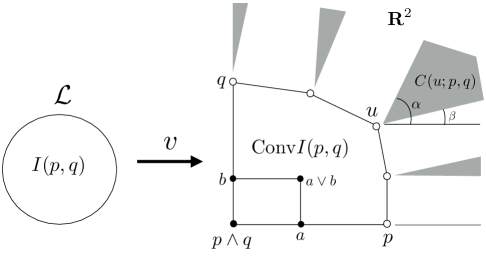
Figure 4: Construction of fractional join

$(p,q)$-envelope.

First we introduce the concept of the $(p,q)$-envelope. Let $(p,q)$ be a pair of elements in ${\cal L}$. Define vector $v(u;p,q)$ in ${\bf R}^{2}_{+}$ by

(3.1) $$v(u;p,q):=(v[p\wedge q,u\wedge p],v[p\wedge q,u\wedge q]).$$

Let $\mathop{\rm Conv}I(p,q)$ denote the convex hull of $\{v(u;p,q)\mid u\in I(p,q)\}$ in ${\bf R}^{2}_{+}$. The polygon $\mathop{\rm Conv}I(p,q)$ contains $v(p\wedge q;p,q)=(0,0)$, $v(p;p,q)=(v[p\wedge q,p],0)$, and $v(q;p,q)=(0,v[p\wedge q,q])$ as extreme points, and contains horizontal segment $[v(p\wedge q;p,q),v(p;p,q)]$ and vertical segment $[v(p\wedge q;p,q),v(q;p,q)]$ as edges. Also $\mathop{\rm Conv}I(p,q)$ is contained in the rectangle of four vertices

$$(0,0),(v[p\wedge q,p],0),(v[p\wedge q,p],0),(v[p\wedge q,p],v[p\wedge q,q]).$$

The $(p,q)$-envelope ${\cal E}({p,q})$ is the set of elements $u\in I(p,q)$ such that $v(u;p,q)$ is a maximal extreme point of $\mathop{\rm Conv}I(p,q)$, where a maximal extreme point is an extreme point $z$ in $\mathop{\rm Conv}I(p,q)$ such that for every positive vector $\epsilon$ it holds $z+\epsilon\not\in\mathop{\rm Conv}I(p,q)$. Observe that ${\cal E}({p,q})$ always contains $p$ and $q$.

Lemma 3.1.

The map $u\mapsto v(u;p,q)$ is injective on ${\cal E}(p,q)$.

This lemma will be proved in Section 3.3.1. Hence the map $u\mapsto v(u;p,q)$ is a bijection between ${\cal E}({p,q})$ and the set of maximal extreme points of $\mathop{\rm Conv}I(p,q)$.

Valuation of convex cones in ${\bf R}^{2}_{+}$.

To define the coefficient, we consider a valuation of convex cones in ${\bf R}^{2}_{+}$. Every closed convex cone $C(\neq\{0\})$ in ${\bf R}^{2}_{+}$ is uniquely represented as

$$C=\{(x,y)\in{\bf R}^{2}_{+}\mid-x\sin\alpha+y\cos\alpha\leq 0,\ -x\sin\beta+y\cos\beta\geq 0\}$$

for some $0\leq\beta\leq\alpha\leq\pi/2$. Define $[C]$ by

(3.2) $$[C]:=\frac{\sin\alpha}{\cos\alpha+\sin\alpha}-\frac{\sin\beta}{\cos\beta+\sin\beta}.$$

For convention, we let $[\{0\}]:=0.$ The following property is easily verified, where $C,C^{\prime}$ are closed convex cones in ${\bf R}^{2}_{+}$:
$(3.3)$ (1) $[C]\geq 0$, and $[C]>0$ if and only if $C$ is full dimensional. (2) $[C]+[C^{\prime}]=[C\cap C^{\prime}]+[C\cup C^{\prime}]$ for $C\cap C^{\prime}\neq\emptyset$. (3) $[{\bf R}^{2}_{+}]=1$.
We are now ready to define the fractional join.

Fractional join.

For $u\in I(p,q)$, let $C(u;p,q)$ denote the set of nonnegative vectors $w\in{\bf R}^{2}_{+}$ with $\langle w,v(u;p,q)\rangle=\max_{u^{\prime}\in I(p,q)}\langle w,v(u^{\prime};p,q)\rangle$, where $\langle,\rangle$ is the standard inner product. Namely $C(u;p,q)$ is the intersection of ${\bf R}^{2}_{+}$ and the normal cone of $\mathop{\rm Conv}I(p,q)$ at extreme point $v(u;p,q)$. In particular, $C(u;p,q)$ forms a closed convex cone in ${\bf R}^{2}_{+}$. The fractional join of $(p,q)$ is the formal convex combination of $u\in{\cal E}(p,q)$ with coefficient $[C(u;p,q)]$:

$$\sum_{u\in{\cal E}(p,q)}[C(u;p,q)]u.$$

Obviously it holds $[C(u;p,q)]=0$ for $u\in I(p,q)\setminus{\cal E}(p,q)$ since $C(u;p,q)=\{0\}$. So the fractional join is also equal to $\sum_{u\in I(p,q)}[C(u;p,q)]u$. Note that the set ${\cal E}(p,q)$ and the coefficient $[C(u_{i};p,q)]$ depend on valuation $v$. Since the set of cones $C(u;p,q)$ $(u\in{\cal E}(p,q))$ forms the intersection of ${\bf R}^{2}_{+}$ and the normal fan of $\mathop{\rm Conv}I(p,q)$, we have
$(3.4)$ (1) ${\bf R}^{2}_{+}=\bigcup_{u\in{\cal E}(p,q)}C(u;p,q)$. (2) For distinct $u,u^{\prime}\in{\cal E}(p,q)$, the intersection $C(u;p,q)\cap C(u^{\prime};p,q)$ has no interior point, and hence $[C(u;p,q)\cap C(u^{\prime};p,q)]=0$. (3) $\bigcup_{u\in{\cal E}(p,q)}[C(u;p,q)]=1$.
Therefore the fractional join of $p,q$ is a formal convex combination of elements in ${\cal E}(p,q)$. An explicit formula of $[C(u;p,q)]$ is given as follows.

Lemma 3.2.

Suppose that ${\cal E}(p,q)=\{p=u_{0},u_{1},u_{2},\ldots,u_{m}=q\}$, and $v(u_{i};p,q)$ and $v(u_{i+1};p,q)$ are adjacent extreme points in $\mathop{\rm Conv}I(p,q)$. Then we have

$$[C(u_{i};p,q)]=\delta_{i}-\delta_{i-1}\quad(i=0,1,2,\ldots,m),$$

where $\delta_{i}$ is defined by $\delta_{-1}:=0$, $\delta_{m}:=1$, and

$$\delta_{i}:=\frac{v[u_{i}\wedge u_{i+1},u_{i}]}{v[u_{i}\wedge u_{i+1},u_{i}]+v[u_{i}\wedge u_{i+1},u_{i+1}]}\quad(i=1,2,\ldots,m-1).$$

This lemma will be proved in Section 3.3.1. We next define the fractional join operation. Let ${\cal O}({\cal L})$ denote the set of all binary operations ${\vartheta}:{\cal L}\times{\cal L}\to{\cal L}$. Regard ${\cal O}({\cal L})$ as a poset by the order: $\vartheta\preceq\vartheta^{\prime}$ if $\vartheta(p,q)\preceq\vartheta^{\prime}(p,q)$ for all $p,q$. Then ${\cal O}({\cal L})$ is isomorphic to the product ${\cal L}^{{\cal L}\times{\cal L}}$ of ${\cal L}$ by the correspondence:

(3.5) $${\cal O}({\cal L})\ni\vartheta\longleftrightarrow(\vartheta(p,q):p,q\in{\cal L})\in{\cal L}^{{\cal L}\times{\cal L}}.$$

In particular ${\cal O}({\cal L})$ is also a modular semilattice, where the meet $\wedge$ is given by $(\vartheta\wedge\vartheta^{\prime})(p,q):=\vartheta(p,q)\wedge\vartheta^{\prime}(p,q)$. The valuation of ${\cal O}({\cal L})$ is given according to (2.10), and is also denoted by $v$. Let $L,R$ be the projection operations defined by

$$L(p,q):=p,\quad R(p,q):=q\quad(p,q\in{\cal L}).$$

Let $I({\cal L}):=I(L,R)$, and let ${\cal E}({\cal L})$ denote the $(L,R)$-envelope ${\cal E}({L,R})$ in ${\cal O}({\cal L})$. An operation in ${\cal E}({\cal L})$ is called extremal. For an operation $\vartheta$ in $I({\cal L})$, the cone $C(\vartheta;L,R)$ is denoted simply by $C({\vartheta})$. The fractional join operation is the formal sum of extremal operations $\vartheta$ with coefficient $[C(\vartheta)]$:

$$\sum_{\vartheta\in{\cal E}({\cal L})}[C(\vartheta)]\vartheta.$$

The fractional join operation is nothing but the fractional join of $L,R$ in ${\cal O}({\cal L})$, and indeed gives fractional joins in ${\cal L}$.

Proposition 3.3.

$\displaystyle\sum_{u\in{\cal E}(p,q)}[C(u;p,q)]u=\sum_{\vartheta\in{\cal E}({\cal L})}[C(\vartheta)]\vartheta(p,q)\quad(p,q\in{\cal L}).$

The proof is given in Section 3.3.2. Consider the case where ${\cal L}$ is the product of modular semilattices ${\cal L}_{i}$ for $i=1,2,\ldots,n$. For operations $\vartheta_{i}$ on ${\cal L}_{i}$ $(i=1,2,\ldots,n)$, the componentwise extension $(\vartheta_{1},\vartheta_{2},\ldots,\vartheta_{n})$ is an operation on ${\cal L}$ defined by

$$(\vartheta_{1},\vartheta_{2},\ldots,\vartheta_{n})(p,q) = (\vartheta_{1}(p_{1},q_{1}),\vartheta_{2}(p_{2},q_{2}),\ldots,\vartheta_{n}(p_{n},q_{n}))$$

$$\quad\quad\quad(p,q\in{\cal L}={\cal L}_{1}\times{\cal L}_{2}\times\cdots\times{\cal L}_{n}).$$

Proposition 3.4.

$$\sum_{\vartheta\in{\cal E}({\cal L})}[C(\vartheta)]\vartheta=\sum_{\vartheta_{1},\vartheta_{2},\ldots,\vartheta_{n}}[C(\vartheta_{1})\cap C(\vartheta_{2})\cap\cdots\cap C(\vartheta_{n})](\vartheta_{1},\vartheta_{2},\ldots,\vartheta_{n}),$$

where $\vartheta_{i}$ is taken over all extremal operations in ${\cal L}_{i}$ $(i=1,2,\ldots,n)$. Moreover, if ${\cal L}_{i}={\cal L}_{j}$ and $\vartheta_{i}\neq\vartheta_{j}$ for some $i,j$, then $[C(\vartheta_{1})\cap C(\vartheta_{2})\cap\cdots\cap C(\vartheta_{n})]=0$.

The proof is given in Section 3.3.3. In particular, any extremal operation $\vartheta$ in ${\cal L}$ is the componentwise extension of extremal operations $\theta_{i}$ in ${\cal L}_{i}$ for $i=1,2,\ldots,n$.

3.2 Submodular function

Let ${\cal L}$ be a modular semilattice with valuation $v$. A function $f:{\cal L}\to\overline{{\bf R}}$ is called submodular on ${\cal L}$ (with respect to $v$) if it satisfies

(3.6) $$f(p)+f(q)\geq f(p\wedge q)+\sum_{u\in{\cal E}(p,q)}[C(u;p,q)]f(u)\quad(p,q\in{\cal L}).$$

By Proposition 3.3, a submodular function may also be characterized as a function $f$ satisfying

(3.7) $$f(p)+f(q)\geq f(p\wedge q)+\sum_{\vartheta\in{\cal E}({\cal L})}[C(\vartheta)]f(\vartheta(p,q))\quad(p,q\in{\cal L}).$$

In the case where a pair $(p,q)$ is bounded, the join $(p,q)$ exists, $\mathop{\rm Conv}I(p,q)$ is a square of vertices $(0,0),(0,v[p\wedge q,q]),(v[p\wedge q,p],0),(v[p\wedge q,p],v[p\wedge q,q])$, ${\cal E}(p,q)=\{p,p\vee q,q\}$, and the fractional join is equal to $0p+1(p\vee q)+0q=p\vee q$. See Figure 5.

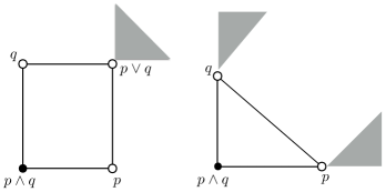
Figure 5: $\mathop{\rm Conv}I(p,q)$ for a bounded pair (left) and an antipodal pair (right)

Hence the corresponding inequality in (3.6) is equal to the usual submodularity inequality:

(3.8) $$f(p)+f(q)\geq f(p\wedge q)+f(p\vee q).$$

Another extremal case is the case of ${\cal E}(p,q)=\{p,q\}$, which implies that $\mathop{\rm Conv}I(p,q)$ is the triangle with vertices $(0,0),(v[p\wedge q,p],0),(0,v[p\wedge q,q])$. Such a pair $(p,q)$ is called antipodal. By definition, a pair $(p,q)$ is antipodal if and only if every bounded pair $(a,b)$ with $p\succeq a\succeq p\wedge q\preceq b\preceq q$ satisfies

(3.9) $$v[a,p]v[b,q]\geq v[p\wedge q,a]v[p\wedge q,b].$$

This condition rephrases that the point $v(a\vee b;p,q)$ is lower than the line through the points $v(p;p,q)$ and $v(q;p,q)$. In this case, the fractional join of $(p,q)$ is equal to

$$\frac{v[p\wedge q,p]}{v[p\wedge q,p]+v[p\wedge q,q]}p+\frac{v[p\wedge q,q]}{v[p\wedge q,p]+v[p\wedge q,q]}q.$$

The inequality in (3.6) corresponds to

(3.10) $$v[p\wedge q,q]f(p)+v[p\wedge q,p]f(q)\geq(v[p\wedge q,p]+v[p\wedge q,q])f(p\wedge q).$$

We call this inequality the $\wedge$-convexity inequality. Then inequalities (3.8) and (3.10) suffice to characterize the submodularity:

Theorem 3.5.

$f:{\cal L}\to\overline{{\bf R}}$ is submodular if and only if it satisfies

• ${\cal E}(p,q)\subseteq\mathop{\rm dom}f$ for $p,q\in\mathop{\rm dom}f$,

• the submodularity inequality for every bounded pair $(p,q)$, and

• the $\wedge$-convexity inequality for every antipodal pair $(p,q)$.

The proof is given in Section 3.3.1. One of the main properties of our submodularity is the following:

Theorem 3.6.

Let ${\cal L}$ be a modular semilattice. The distance function $d_{{\cal L}}$ on ${\cal L}$ is submodular on ${\cal L}\times{\cal L}$.

We will prove this theorem and a more general version (Theorem 4.8) in Section 4.3.3. We note some basic properties of our submodular functions concerning addition and restriction.

Lemma 3.7.

Let ${\cal L},{\cal L}^{\prime},{\cal M}$ and ${\cal M}^{\prime}$ be modular semilattices, and let $f$ and $f^{\prime}$ be submodular functions on ${\cal L}$.

• For $b\in{\bf R}$ and $c,c^{\prime}\in{\bf R}_{+}$, $b+cf+c^{\prime}f^{\prime}$ is a submodular function on ${\cal L}$.

• A function $\tilde{f}$ defined by

  $$\tilde{f}(p,p^{\prime}):=f(p)\quad((p,p^{\prime})\in{\cal L}\times{\cal L}^{\prime})$$

  is a submodular function on ${\cal L}\times{\cal L}^{\prime}$.

• Suppose ${\cal L}={\cal M}\times{\cal M}^{\prime}$. For any $p^{\prime}\in{\cal M}^{\prime}$, a function $f_{p^{\prime}}$ defined by

  $$f_{p^{\prime}}(p):=f(p,p^{\prime})\quad(p\in{\cal M})$$

  is a submodular function on ${\cal M}$.

• For a convex set ${\cal N}$ of ${\cal L}$, the restriction of $f$ to ${\cal N}$ is a submodular function on ${\cal N}$ (regarded as a modular semilattice).

Proof.

(1) follows from the facts that the submodularity is closed under nonnegative sum, and that any constant function is submodular (by ((3)) (3)).

(2) follows from (3.7), Proposition 3.4, and

$$\tilde{f}(p,p^{\prime})+\tilde{f}(q,q^{\prime})=f(p)+f(q)\geq f(p\wedge q)+\sum_{\vartheta\in{\cal E}({\cal L})}[C(\vartheta)]f(\vartheta(p,q))$$

$$=\tilde{f}(p\wedge q,p^{\prime}\wedge q^{\prime})+\sum_{\vartheta\in{\cal E}({\cal L})}\sum_{\vartheta^{\prime}\in{\cal E}({\cal L}^{\prime})}[C(\vartheta)\cap C(\vartheta^{\prime})]\tilde{f}(\vartheta(p,q),\vartheta^{\prime}(p^{\prime},q^{\prime})),$$

where we use $[C(\vartheta)]=\sum_{\vartheta^{\prime}\in{\cal E}({\cal L}^{\prime})}[C(\vartheta)\cap C(\vartheta^{\prime})]$ (obtained from ((3))).

(3). Notice that the $(p,p)$-envelope is $\{p\}$, and any extremal operation $\vartheta$ is idempotent, i.e., $\vartheta(p,p)=p$. Thus, by Proposition 3.4, we have

$$f_{p^{\prime}}(p)+f_{p^{\prime}}(q)=f(p,p^{\prime})+f(q,p^{\prime})$$

$$\geq f(p\wedge q,p^{\prime}\wedge p^{\prime})+\sum_{\vartheta\in{\cal E}({\cal M})}\sum_{\vartheta^{\prime}\in{\cal E}({\cal M^{\prime}})}[C(\vartheta)\cap C(\vartheta^{\prime})]f(\vartheta(p,q),\vartheta^{\prime}(p^{\prime},p^{\prime}))$$

$$=f(p\wedge q,p^{\prime})+\sum_{\vartheta\in{\cal E}({\cal M})}\sum_{\vartheta^{\prime}\in{\cal E}({\cal M^{\prime}})}[C(\vartheta)\cap C(\vartheta^{\prime})]f(\vartheta(p,q),p^{\prime})$$

$$=f_{p^{\prime}}(p\wedge q)+\sum_{\vartheta\in{\cal E}({\cal M})}[C(\vartheta)]f_{p^{\prime}}(\vartheta(p,q)).$$

(4) follows from the fact that for $p,q\in{\cal N}$ the metric interval $I(p,q)$ is the same on ${\cal L}$ and on ${\cal N}$. ∎

We finally give a useful criterion of the submodularity. A bounded pair $(p,q)$ in ${\cal L}$ is said to be $2$-bounded if $p\vee q$ covers $p$ and $q$ (in which case both $p$ and $q$ cover $p\wedge q$).

Proposition 3.8.

Suppose that ${\cal L}$ is the product of two modular semilattices ${\cal L}_{1}\times{\cal L}_{2}$. $f:{\cal L}\to{\bf R}$ is submodular if and only if it satisfies

• the submodularity inequality for every $2$-bounded pair $p,q$, and

• the $\wedge$-convexity inequality for every pair $(p,q)=((p_{1},p_{2}),(q_{1},q_{2}))$ such that $p_{1}=q_{1}$ and $(p_{2},q_{2})$ is antipodal in ${\cal L}_{2}$ or $p_{2}=q_{2}$ and $(p_{1},q_{1})$ is antipodal in ${\cal L}_{1}$.

The proof is given in Section 3.3.4. Notice that this criterion does not work when $f$ has infinite values.

Minimizing a sum of submodular functions with bounded arity.

Here we consider the problem of minimizing submodular function $f$ on the product of modular semilattices ${\cal L}_{1},{\cal L}_{2},\ldots,{\cal L}_{n}$, where the input of the problem is ${\cal L}_{1},{\cal L}_{2},\ldots,{\cal L}_{n}$ and an evaluating oracle of $f$. In the case where each ${\cal L}_{i}$ is a lattice of rank $1$, this problem is the submodular set function minimization in the ordinary sense, and can be solved in polynomial time [20, 30, 54]. However, we do not know whether this problem in general is polynomial time solvable or not. One notable result in this direction, due to Kuivinen [43], is that if each ${\cal L}_{i}$ is a complemented modular lattice of rank $2$ (a diamond lattice), then this problem has a good characterization.

So we restrict our investigation to the problem of minimizing a sum of submodular functions with bounded arity, i.e., valued CSP for submodular functions. See Section 2.1 for notions in valued CSP. Let ${\cal L}:={\cal L}_{1}\times{\cal L}_{2}\times\cdots\times{\cal L}_{n}$. A constraint $f$ on ${\cal L}$ is called submodular if $f$ is a submodular function on ${\cal L}_{I_{f}}$. The submodular language ${\cal S}_{\cal L}$ is the set of all submodular constraints on ${\cal L}$.

Theorem 3.9.

Let ${\cal L}$ be the product of modular semilattices ${\cal L}_{1},{\cal L}_{2},\ldots,{\cal L}_{n}$. Then VCSP$[{\cal S}_{\cal L}]$ can be solved in polynomial time.

Indeed, the submodular language ${\cal S}_{\cal L}$ satisfies the Thapper-Živný criterion (Theorem 2.1). Define a fractional operation $\omega$ on ${\cal L}$ by

(3.11) $$\omega=\frac{1}{2}\wedge+\frac{1}{2}\sum_{\vartheta\in{\cal E}({\cal L})}[C(\vartheta)]\vartheta.$$

By Proposition 3.4, an extremal operation is the componentwise extension of operations in ${\cal L}_{i}$, and is separable. Also, by ((3)) (3), the total sum of coefficients $[C(\vartheta)]$ is equal to $1$. Therefore $\omega$ is a fractional polymorphism for the submodular language ${\cal S}_{\cal L}$. Obviously $\wedge$ is a semilattice operation. Hence Theorem 3.9 follows from Theorem 2.1.

Figure 6: A nonsemilattice orientable modular graph

Remark 3.10.

Suppose that ${\mit\Gamma}$ is the covering graph of a modular semilattice ${\cal L}$. By Theorem 3.6 and Lemma 3.7, $g_{j}$ and $f_{ij}$ (defined in (2.1)) are submodular constraints on ${\cal L}^{n}$. Then 0-Ext$[{\mit\Gamma}]$ is a subclass of VCSP$[{\cal S}_{{\cal L}^{n}}]$. Therefore, by Theorem 3.9, 0-Ext$[{\mit\Gamma}]$ can be solved by the basic LP relaxation. This observation, however, does not get us to the main result (Theorem 1.6) since there is an orientable modular graph that cannot be represented as the covering graph of a modular semilattice. See the graph of Figure 6, where there are exactly two admissible orientations: one is the reverse of the other, and both orientations have two sinks and two sources. Nevertheless, the basic LP is expected to solve 0-Ext$[{\mit\Gamma}]$ for an arbitrary orientable modular graph ${\mit\Gamma}$; see Section 6.

3.3 Proofs

3.3.1 Proof of Lemmas 3.1 and 3.2 and Theorem 3.5

Let $(p,q)$ be a pair of elements in modular semilattice ${\cal L}$. First we prove a general version of Lemma 3.1.

Lemma 3.11.

For $s,s^{\prime}\in{\cal E}(p,q)$, if $v(s\wedge p)\geq v(s^{\prime}\wedge p)$ and $v(s\wedge q)\leq v(s^{\prime}\wedge q)$, then $s\wedge p\succeq s^{\prime}\wedge p$ and $s\wedge q\preceq s^{\prime}\wedge q$. In particular, $v(s;p,q)=v(s^{\prime};p,q)$ implies $s=s^{\prime}$.

Proof.

We can assume that $v(p\wedge q)=0$ by adding a constant to $v$ (for notational simplicity). It suffices to consider the case where $v(s;p,q)=v(s^{\prime};p,q)$ or $v(s;p,q)$ and $v(s^{\prime};p,q)$ are adjacent extreme points in $\mathop{\rm Conv}I(p,q)$. Let $(a,b):=(s\wedge p,s\wedge q)$ and $(a^{\prime},b^{\prime}):=(s^{\prime}\wedge p,s^{\prime}\wedge q)$. All pairs $(a,a^{\prime})$, $(a,b\wedge b^{\prime})$, and $(a^{\prime},b\wedge b^{\prime})$ from among the triple $(a,a^{\prime},b\wedge b^{\prime})$ are bounded. By definition of modular semilattices, their join $\eta:=(a\vee a^{\prime})\vee(b\wedge b^{\prime})$ exists and belongs to $I(p,q)$ (see Lemma 2.15). Similarly the join $\xi:=(a\wedge a^{\prime})\vee(b\vee b^{\prime})$ of triple $(a\wedge a^{\prime},b,b^{\prime})$ exists and belongs to $I(p,q)$. Therefore $v(\eta;p,q)=(v(a\vee a^{\prime}),v(b\wedge b^{\prime}))$ and $v(\xi;p,q)=(v(a\wedge a^{\prime}),v(b\vee b^{\prime}))$. By modularity equality (2.7) for $v$, we have

$$v(s;p,q)+v(s^{\prime};p,q)=(v(a)+v(a^{\prime}),v(b)+v(b^{\prime}))=v(\eta;p,q)+v(\xi;p,q).$$

Then both $v(\eta;p,q)$ and $v(\xi;p,q)$ must belong to $[v(u;p,q),v(u^{\prime};p,q)]$ since it is an edge (or an extreme point) of $\mathop{\rm Conv}I(p,q)$. Necessarily $v(\eta;p,q)=v(s;p,q)$ and $v(\xi;p,q)=v(s^{\prime};p,q)$. This means that $a\vee a^{\prime}=a$ and $b\vee b^{\prime}=b^{\prime}$. Hence the claim follows. ∎

Lemma 3.12.

For $s,t\in{\cal E}(p,q)$ with $t\wedge p\preceq s\wedge p$ (and $t\wedge q\succeq s\wedge q$), the following hold:

• $d(p,q)=d(p,s)+d(s,t)+d(t,q)$; in particular $I(s,t)\subseteq I(p,q)$.

• $v(u;p,q)=v(u;s,t)+v(s\wedge t;p,q)$ for $u\in I(s,t)\subseteq I(p,q)$.

• If $v(s;p,q)$ and $v(t;p,q)$ are adjacent extreme points, then $(s,t)$ is antipodal.

Proof.

(1). By Lemma 2.15 (4), we have $(s\wedge t)\vee(q\wedge t)=(s\wedge t\wedge p)\vee(s\wedge t\wedge q)\vee(q\wedge t)=(t\wedge p)\vee(t\wedge q)=t$. This means $t\in I(s,q)$. Hence $d(p,q)=d(p,s)+d(s,q)=d(p,s)+d(s,t)+d(t,q)$.

(2). By $u\wedge s=(s\wedge t)\vee(u\wedge p)$ (Lemma 2.15 (4) for $I(p,t)$), we have $v[t\wedge p,p\wedge u]=v[s\wedge t,u\wedge s]$, and

$$v[p\wedge q,p\wedge u]=v[p\wedge q,t\wedge p]+v[t\wedge p,p\wedge u]=v[p\wedge q,s\wedge t\wedge p]+v[s\wedge t,u\wedge s].$$

Similarly (for $I(s,q)$), we have $v[p\wedge q,q\wedge u]=v[p\wedge q,s\wedge t\wedge q]+v[s\wedge t,u\wedge t]$.

(3). If $(s,t)$ is not antipodal, then there is $u\in I(s,t)$ such that $v(u;s,t)$ goes beyond the line segment between $v(s;s,t)$ and $v(t;s,t)$. Then, by (2), $v(u;p,q)$ is in the outside of $\mathop{\rm Conv}I(p,q)$. This is a contradiction. ∎

Suppose that ${\cal E}({p,q})=\{p=u_{0},u_{1},\ldots,u_{m}=q\}$, and $v(u_{i};p,q)$ and $v(u_{i+1};p,q)$ are adjacent extreme points. Let $\theta_{i}$ be the angle of the line normal to the line segment connecting $v(u_{i-1};p,q)$ and $v(u_{i};p,q)$. By Lemma 3.12 (2), $\theta_{i}$ is equal to the angle of the line normal to the line segment connecting $v(u_{i-1};u_{i},u_{i-1})$ and $v(u_{i};u_{i},u_{i-1})$. Therefore

(3.12) $$\frac{\sin\theta_{i}}{\sin\theta_{i}+\cos\theta_{i}}=\frac{v[u_{i}\wedge u_{i-1},u_{i-1}]}{v[u_{i}\wedge u_{i-1},u_{i-1}]+v[u_{i}\wedge u_{i-1},u_{i}]}=\delta_{i-1}.$$

Therefore we obtain the formula of Lemma 3.2.

Next we prove Theorem 3.5. It suffices to prove the if part. Let $(p,q)$ be a pair of (incomparable) elements in ${\cal L}$. Suppose that ${\cal E}({p,q})=\{p=u_{0},u_{1},\ldots,u_{m}=q\}$ is given as above. Let $p_{i}:=u_{i}\wedge p$ and $q_{i}:=u_{i}\wedge q$ for $i=0,1,2,\ldots,m$. By Lemma 3.11, it holds $p_{i}\succeq p_{j}$ and $q_{i}\preceq q_{j}$ for $i\leq j$.

Figure 7: $\mathop{\rm Conv}I(p,q)$ and ${\cal E}(p,q)$

Let $b_{i}:=u_{i-1}\wedge u_{i}$ for $i=1,2,\ldots,m$; see Figure 7. Then we have

(3.13) $$b_{i}\wedge q_{i}=u_{i-1}\wedge u_{i}\wedge u_{i}\wedge q=q_{i-1}.$$

Also, by Lemma 2.15 (3) and (4), we have

$$b_{i}\vee q_{i} = (u_{i-1}\wedge u_{i})\vee q_{i}=(u_{i-1}\wedge u_{i}\wedge p)\vee(u_{i-1}\wedge u_{i}\wedge q)\vee q_{i}$$

$$= (p_{i-1}\wedge p_{i})\vee(q_{i-1}\wedge q_{i})\vee q_{i}=p_{i}\vee q_{i}=u_{i}.$$

Let $f$ be a function on ${\cal L}$ satisfying the conditions (1), (2), and (3) in Theorem 3.5. We show that $f$ satisfies the inequality (3.6) for $p,q$. We may assume that $p,q\in\mathop{\rm dom}f$. By condition (1), ${\cal E}(p,q)\subseteq\mathop{\rm dom}f$. Namely $u_{i}\in\mathop{\rm dom}f$. By (3), we have $b_{i}=u_{i}\wedge u_{i-1}\in\mathop{\rm dom}f$. By (2), we have $b_{i}\wedge b_{i-1}=u_{i}\wedge u_{i-1}\wedge u_{i-2}=u_{i}\wedge u_{i-2}\in\mathop{\rm dom}f$. Consequently all $p_{i},q_{i},b_{i}$ belong to $\mathop{\rm dom}f$. By (3.13), (3.3.1), and the condition (2) (submodularity), we have

(3.15) $$f(b_{i})+f(q_{i})\geq f(q_{i-1})+f(u_{i})\quad(i=1,2,\ldots,m).$$

By adding (3.15) for $i=1,2,\ldots,m$ and $f(p)=f(u_{0})$ (recall $(p,q)=(u_{0},q_{m})$), we obtain

(3.16) $$f(p)+f(b_{1})+f(b_{2})+\cdots+f(b_{m})+f(q)\geq f(p\wedge q)+f(u_{0})+f(u_{1})+\cdots+f(u_{m}).$$

By Lemma 3.12 (3), pair $(u_{i},u_{i+1})$ is antipodal. By condition (3), $f$ satisfies the $\wedge$-convexity inequality (3.10) for $(u_{i},u_{i+1})$, which is rewritten as

(3.17) $$f(u_{i})\geq f(b_{i+1})+\delta_{i}f(u_{i})-\delta_{i}f(u_{i+1}).$$

Substituting (3.17) to (3.16) for $i=0,1,2,\ldots,m-1$, we obtain

$$f(p)+f(q)\geq f(p\wedge q)+\sum_{i=0}^{m}(\delta_{i}-\delta_{i-1})f(u_{i})=f(p\wedge q)+\sum_{i=0}^{m}[C(u_{i};p,q)]f(u_{i}).$$

3.3.2 Proof of Proposition 3.3

We start with preliminary arguments. Suppose that ${\cal L}$ is the product ${\cal L}_{1}\times{\cal L}_{2}$ of modular semilattices ${\cal L}_{1}$ and ${\cal L}_{2}$. The valuations of ${\cal L}_{1}$ and ${\cal L}_{2}$ are given as (2.8). They are also denoted by $v$. Let $(p,q)=((p_{1},p_{2}),(q_{1},q_{2}))$ be a pair of elements in ${\cal L}$. By (2.9), we have

(3.18) $$v(u;p,q)=v(u_{1};p_{1},q_{1})+v(u_{2};p_{2},q_{2})\quad(u\in I(p,q)).$$

By this equation together with $I(p,q)=I(p_{1},q_{1})\times I(p_{2},q_{2})$, we have

(3.19) $$\mathop{\rm Conv}I(p,q)=\mathop{\rm Conv}I(p_{1},q_{1})+\mathop{\rm Conv}I(p_{2},q_{2}),$$

where the sum means the Minkowski sum.

In general, if a polytope $P$ is the Minkowski sum of two polytopes $Q$ and $Q^{\prime}$, then every extreme point of $P$ is uniquely represented as the sum of extreme points of $Q$ and of $Q^{\prime}$. By this fact and the injectivity of $v(\cdot;p,q)$ (Lemma 3.1) on ${\cal E}(p,q)$, we obtain:
$(3.20)$    For $u=(u_{1},u_{2})\in{\cal E}(p,q)$, there uniquely exist maximal extreme points $x_{i}\in\mathop{\rm Conv}I(p_{i},q_{i})$ for $i=1,2$ such that $x_{i}=v(u_{i};p_{i},q_{i})$ for $i=1,2$, and $v(u;p,q)=x_{1}+x_{2}$. In particular, $u_{i}$ belongs to ${\cal E}(p_{i},q_{i})$ for $i=1,2$.
Moreover, $v(u;p,q)$ maximizes $\langle c,x\rangle$ over $x\in\mathop{\rm Conv}I(p,q)$ if and only if $v(u_{i};p_{i},q_{i})$ maximizes $\langle c,x\rangle$ over $x\in\mathop{\rm Conv}I(p_{i},q_{i})$ for $i=1,2$. Therefore we have

(3.21) $$C(u;p,q)=C(u_{1};p_{1},q_{1})\cap C(u_{2};p_{2},q_{2}).$$

We are ready to prove Proposition 3.3. Regard ${\cal O}({\cal L})$ as a modular semilattice ${\cal L}^{{\cal L}\times{\cal L}}$. Then $I({\cal L})$ is the product of $I(L(p,q),R(p,q))=I(p,q)$ over all $(p,q)\in{\cal L}\times{\cal L}$. By (3.19) we have

$$\mathop{\rm Conv}I({\cal L})=\sum_{(p,q)\in{\cal L}\times{\cal L}}\mathop{\rm Conv}I(p,q).$$

By (3.3.2), for every extremal operation $\vartheta$, each $\vartheta(p,q)$ belongs to ${\cal E}(p,q)$. Also, by (3.21), we have

(3.22) $$C(\vartheta)=\bigcap_{(p,q)\in{\cal L}\times{\cal L}}C(\vartheta(p,q);p,q)\quad(\vartheta\in{\cal E}({\cal L})).$$

From ((3)), $C(\vartheta)\subseteq C(u;p,q)$ if and only if $\vartheta(p,q)=u$, and

(3.23) $$C(u;p,q)=\bigcup_{\vartheta\in{\cal E}({\cal L}):\vartheta(p,q)=u}C(\vartheta)\quad(p,q\in{\cal L},u\in{\cal E}(p,q)),$$

where any two of the cones in the union have no common interior points. Therefore

$$\sum_{\vartheta\in{\cal E}({\cal L})}[C(\vartheta)]\vartheta(p,q)=\sum_{u\in{\cal E}(p,q)}\left(\sum_{\vartheta\in{\cal E}({\cal L}):\vartheta(p,q)=u}[C(\vartheta)]\right)u=\sum_{u\in{\cal E}(p,q)}[C(u;p,q)]u.$$

This proves Proposition 3.3.

3.3.3 Proof of Proposition 3.4

It suffices to consider the case where ${\cal L}={\cal L}_{1}\times{\cal L}_{2}$. If $\vartheta\in I({\cal L})$ is the componentwise extension of $\vartheta_{i}\in I({\cal L}_{i})$ for $i=1,2$, then

$$v(\vartheta;L,R) = \sum_{(p,q)\in{\cal L}\times{\cal L}}v(\vartheta(p,q);p,q)$$

$$= \sum_{(p,q)\in{\cal L}\times{\cal L}}v(\vartheta_{1}(p_{1},q_{1});p_{1},q_{1})+v(\vartheta_{2}(p_{2},q_{2});p_{2},q_{2})$$

$$= |{\cal L}_{2}|^{2}v(\vartheta_{1};L,R)+|{\cal L}_{1}|^{2}v(\vartheta_{2};L,R).$$

Therefore it holds

(3.25) $$\mathop{\rm Conv}I({\cal L})\supseteq|{\cal L}_{2}|^{2}\mathop{\rm Conv}I({\cal L}_{1})+|{\cal L}_{1}|^{2}\mathop{\rm Conv}I({\cal L}_{2}).$$

We are going to show that every extremal operation in ${\cal L}$ is the componentwise extension of operations in ${\cal L}_{i}$ for $i=1,2$, and the equality holds in (3.25). Take an extremal operation $\vartheta$ on ${\cal L}$. There are $\vartheta_{i}:{\cal L}\times{\cal L}\to{\cal L}_{i}$ for $i=1,2$ such that $\vartheta(p,q)=(\vartheta_{1}(p,q),\vartheta_{2}(p,q))$ for $(p,q)\in{\cal L}\times{\cal L}$. By Proposition 3.3, $\vartheta(p,q)$ belongs to ${\cal E}(p,q)$. By (3.3.2), $\vartheta_{1}(p,q)$ and $\vartheta_{2}(p,q)$ belong to ${\cal E}(p_{1},q_{1})$ and ${\cal E}(p_{2},q_{2})$, respectively. For $(p,q),(p^{\prime},q^{\prime})\in{\cal L}\times{\cal L}$ with $(p_{1},q_{1})=(p^{\prime}_{1},q^{\prime}_{1})$, suppose (indirectly) that $\vartheta_{1}(p,q)\neq\vartheta_{1}(p^{\prime},q^{\prime})$. Let $\vartheta^{\prime}$ be the operation in $I({\cal L})$ obtained from $\vartheta$ by replacing $\vartheta_{1}(p^{\prime},q^{\prime})$ with $\vartheta_{1}(p,q)$, and let $\vartheta^{\prime\prime}$ be the operation in $I({\cal L})$ obtained from $\vartheta$ by replacing $\vartheta_{1}(p,q)$ with $\vartheta_{1}(p^{\prime},q^{\prime})$. Then we have

$$v(\vartheta(p,q);p,q)+v(\vartheta(p^{\prime},q^{\prime});p^{\prime},q^{\prime})=\sum_{i=1,2}v(\vartheta_{i}(p,q);p_{i},q_{i})+v(\vartheta_{i}(p^{\prime},q^{\prime});p^{\prime}_{i},q^{\prime}_{i})$$

$$=\frac{1}{2}\left\{(v(\vartheta^{\prime}(p,q);p,q)+v(\vartheta^{\prime}(p^{\prime},q^{\prime});p^{\prime},q^{\prime}))+(v(\vartheta^{\prime\prime}(p,q);p,q)+v(\vartheta^{\prime\prime}(p^{\prime},q^{\prime});p^{\prime},q^{\prime}))\right\}.$$

By Lemma 3.1, $v(\vartheta_{1}(p,q);p_{1},q_{1})$ and $v(\vartheta_{1}(p^{\prime},q^{\prime});p_{1},q_{1})$ are distinct, and consequently $v(\vartheta;L,R)$ is the midpoint of segment between distinct points $v(\vartheta^{\prime};L,R)$ and $v(\vartheta^{\prime\prime};L,R)$, contradicting the fact that $\vartheta$ is extremal. Therefore $\vartheta_{1}(p,q)=\vartheta_{1}(p^{\prime},q^{\prime})$ must hold. This means that $\vartheta_{1}(p,q)$ does not depend on the second component of each of $p,q$. So we can regard $\vartheta_{1}\in I({\cal L}_{1})$. Similarly $\vartheta_{2}\in I({\cal L}_{2})$, and $\vartheta$ is equal to the componentwise extension of $\vartheta_{1}$ and $\vartheta_{2}$. Hence the equality holds in (3.25), both $\vartheta_{1}$ and $\vartheta_{2}$ must be extremal, and $[C(\vartheta)]=[C(\vartheta_{1})\cap C(\vartheta_{2})]$. Thus we have

$$\sum_{\vartheta\in{\cal E}({\cal L})}[C(\vartheta)]\vartheta=\sum_{\vartheta_{1}\in{\cal E}({\cal L}_{1}),\vartheta_{2}\in{\cal E}({\cal L}_{2})}[C(\vartheta_{1})\cap C(\vartheta_{2})](\vartheta_{1},\vartheta_{2}).$$

Suppose that ${\cal L}_{1}={\cal L}_{2}$ holds. Suppose that $\vartheta_{1}$ and $\vartheta_{2}$ are different. We see from (3.3.3) that $v((\vartheta_{1},\vartheta_{2});L,R)$ is the midpoint of the segment between distinct points $v((\vartheta_{1},\vartheta_{1});L,R)$ and $v((\vartheta_{2},\vartheta_{2});L,R)$. Hence $(\vartheta_{1},\vartheta_{2})$ is never extremal. The proof of Proposition 3.4 is now complete.

3.3.4 Proof of Proposition 3.8

We use the characterization of Theorem 3.5. So the only if part is obvious. We prove the if part. We first show that the submodularity inequality for an arbitrary bounded pair is implied by submodularity inequalities for $2$-bounded pairs. For a bounded pair $(p,q)$, take maximal chains $(p\wedge q=p_{0},p_{1},\ldots,p_{k}=p)$ and $(p\wedge q=q_{0},q_{1},\ldots,q_{l}=q)$. Let $a_{i,j}:=p_{i}\vee q_{j}$. Then $f(p)+f(q)-f(p\wedge q)-f(p\vee q)=\sum_{i,j}(f(a_{i+1,j})+f(a_{i,j+1})-f(a_{i+1,j+1})-f(a_{i,j}))\geq 0$. Here we use the fact seen from modularity that $(a_{i+1,j},a_{i,j+1})$ is a $2$-bounded pair with $a_{i+1,j+1}=a_{i+1,j}\vee a_{i,j+1}$ and $a_{i,j}=a_{i+1,j}\wedge a_{i,j+1}$.

Next we show the $\wedge$-convexity inequality. Take an (incomparable) antipodal pair $(p,q)=((p_{1},p_{2}),(q_{1},q_{2}))$ in ${\cal L}$. Then ${\cal E}({p,q})=\{p,q\}$. Then $\mathop{\rm Conv}I(p,q)$ is a triangle. By (3.19), it holds $\mathop{\rm Conv}I(p,q)=\mathop{\rm Conv}I(p_{1},q_{1})+\mathop{\rm Conv}I(p_{2},q_{2})$. Therefore both $\mathop{\rm Conv}I(p_{1},q_{1})$ and $\mathop{\rm Conv}I(p_{2},q_{2})$ are triangles congruent to a dilation of $\mathop{\rm Conv}I(p,q)$. Hence $(p_{i},q_{i})$ is antipodal in ${\cal L}_{i}$, and $C(p_{i};p_{i},q_{i})=C(p;p,q)$ and $C(q_{i};p_{i},q_{i})=C(q;p,q)$ for $i=1,2$. In particular, both $((q_{1},q_{2}),(q_{1},p_{2}))$ and $((q_{1},p_{2}),(p_{1},p_{2}))$ are antipodal pairs in ${\cal L}={\cal L}_{1}\times{\cal L}_{2}$. Letting $C_{p}:=C(p;p,q)=C(p_{i};p_{i},q_{i})$ and $C_{q}:=C(q;p,q)=C(q_{i};p_{i},q_{i})$, we have

$$(1-[C_{q}])f(q_{1},q_{2})+(1-[C_{p}])f(q_{1},p_{2})\geq f(q_{1},p_{2}\wedge q_{2}),$$

$$(1-[C_{q}])f(q_{1},p_{2})+(1-[C_{p}])f(p_{1},p_{2})\geq f(p_{1}\wedge q_{1},p_{2}).$$

Also, by submodularity inequality (shown above), we have

$$f(q_{1},p_{2}\wedge q_{2})+f(p_{1}\wedge q_{1},p_{2})\geq f(p_{1}\wedge q_{1},p_{2}\wedge q_{2})+f(q_{1},p_{2}).$$

From the three inequalities, we obtain

$$(1-[C_{q}])f(q_{1},q_{2})+(2-[C_{p}]-[C_{q}])f(q_{1},p_{2})+(1-[C_{p}])f(p_{1},p_{2})$$

$$\quad\quad\geq f(p_{1}\wedge q_{1},p_{2}\wedge q_{2})+f(q_{1},p_{2}).$$

By using $[C_{p}]+[C_{q}]=1$, we obtain the $\wedge$-convexity inequality for $(p,q)$.

4 L-convex function on modular complex

A modular complex $\boldsymbol{{\mit\Gamma}}$ is a triple $({\mit\Gamma},o,h)$ of an orientable modular graph ${\mit\Gamma}$, its admissible orientation $o$, and its positive orbit-invariant function $h$. The goal of this section is to introduce a class of discrete convex functions, called L-convex functions, on $\boldsymbol{{\mit\Gamma}}$, and show that L-convex functions have several nice properties for optimization, analogous to L^♮-convex functions in discrete convex analysis.

The main properties of our L-convex functions are:

• The distance function $d_{{{\mit\Gamma}},h}$ is an L-convex function on $\boldsymbol{{\mit\Gamma}}\times\boldsymbol{{\mit\Gamma}}$ (Theorem 4.8).

• In the minimization of an L-convex function, checking optimality and finding a descent direction can be done by submodular function minimization on modular semilattices (Theorem 4.11).

In Section 4.1, we explore several structural properties of modular complexes. In particular, a modular complex can be regarded as a structure obtained by gluing modular semilattices (Theorem 4.2), and admits a subdivision operation (Theorem 4.3). This operation produces a fine modular complex $\boldsymbol{{\mit\Gamma}}^{*}$ into which the original modular complex $\boldsymbol{{\mit\Gamma}}$ is embedded, and also enables us to define the neighborhood semilattice ${\cal L}_{p}^{*}$ around each vertex $p$, which is also a modular semilattice. Based on this investigation as well as the idea mentioned in the introduction, in Section 4.2, we introduce L-convex functions on $\boldsymbol{{\mit\Gamma}}$, and present their properties. Again less obvious theorems will be proved in Section 4.3. A further geometric study on orientable modular graphs is given in [10].

4.1 Modular complex

Let $\boldsymbol{{\mit\Gamma}}=({\mit\Gamma},o,h)$ be a modular complex, where a modular complex is denoted by the bold style $\boldsymbol{{\mit\Gamma}}$ of the underlying graph ${\mit\Gamma}$.

Boolean pairs.

Consider a cube subgraph $B$ of ${{\mit\Gamma}}$, and consider the digraph $\vec{B}$ of $B$ oriented by $o$. One can easily see from the definition of an admissible orientation that $\vec{B}$ is isomorphic to the Hasse diagram of a Boolean lattice. Hence $\vec{B}$ determines the maximum element and the minimum element of the corresponding Boolean lattice. A pair $(p,q)$ of vertices is called $o$-Boolean, or simply, Boolean if $p$ and $q$ are the minimum element and the maximum element, respectively, of the Boolean lattice associated with some cube subgraph of ${{\mit\Gamma}}$. By convention, $(p,p)$ is defined to be Boolean. The set of Boolean pairs is denoted by ${\cal B}(\boldsymbol{{\mit\Gamma}})$. In Figure 2 in the introduction, for example, $(p^{\prime},p)$, $(v,q)$, $(p^{\prime},v)$ are Boolean, and $(q,p^{\prime})$ is not Boolean.

Recall that any admissible orientation is acyclic (Lemma 2.4). Let $\preceq(=\ \preceq_{o})$ be the transitive closure of relation $\swarrow(=\ \swarrow_{o})$ on $V_{{\mit\Gamma}}$. Then $V_{{\mit\Gamma}}$ is regarded as a partially ordered set according to this relation; so $p\swarrow q$ implies $p\prec q$. For any Boolean pair $(p,q)$, necessarily $p\preceq q$ holds.

Proposition 4.1.

Let $\boldsymbol{{\mit\Gamma}}$ be a modular complex. For $p,q\in V_{{\mit\Gamma}}$ with $p\preceq q$, we have the following:

• $[p,q]$ is a modular lattice, is convex in ${\mit\Gamma}$, and is equal to $I(p,q)$.

• $(p,q)$ is Boolean if and only if $[p,q]$ is a complemented modular lattice.

In particular we can check whether a given pair is Boolean in time polynomial in $|V_{{\mit\Gamma}}|$.

We prove this proposition in Section 4.3.1. We define the relation $\sqsubseteq(=\ \sqsubseteq_{o})$ as: $p\sqsubseteq q$ if $(p,q)$ is a Boolean pair. This relation $\sqsubseteq$ coarsens $\preceq$, and is not transitive in general. Since a complemented modular lattice is relatively complemented (Theorem 2.11), we have:
$(4.1)$    If $p\sqsubseteq q$ and $p\preceq u\preceq v\preceq q$, then $p\sqsubseteq u\sqsubseteq v\sqsubseteq q$.
For a vertex $p$, define subsets ${\cal L}^{+}_{p}(\boldsymbol{{\mit\Gamma}})$ and ${\cal L}^{-}_{p}(\boldsymbol{{\mit\Gamma}})$ of vertices by

(4.2) $${\cal L}^{+}_{p}(\boldsymbol{{\mit\Gamma}}):=\{q\in V_{{\mit\Gamma}}\mid p\sqsubseteq q\},\quad{\cal L}^{-}_{p}(\boldsymbol{{\mit\Gamma}}):=\{q\in V_{{\mit\Gamma}}\mid q\sqsubseteq p\}.$$

In the sequel, ${\cal L}^{+}_{p}(\boldsymbol{{\mit\Gamma}})$ and ${\cal L}^{-}_{p}(\boldsymbol{{\mit\Gamma}})$ are often denoted by ${\cal L}^{+}_{p}$ and ${\cal L}^{-}_{p}$, respectively. Regard ${\cal L}^{+}_{p}$ as a poset by the partial order $\preceq$, and regard ${\cal L}^{-}_{p}$ as a poset by the reverse of $\preceq$.

Theorem 4.2.

Let $\boldsymbol{{\mit\Gamma}}$ be a modular complex. For every vertex $p$, both ${\cal L}^{+}_{p}$ and ${\cal L}^{-}_{p}$ are complemented modular semilattices, and convex in ${\mit\Gamma}$.

Theorem 4.2 will be proved in Section 4.3.1. Therefore $\boldsymbol{{\mit\Gamma}}$ is a structure obtained by gluing modular lattices and semilattices. Moreover $\boldsymbol{{\mit\Gamma}}$ gives rise to a simplicial complex ${\mit\Delta}(\boldsymbol{{\mit\Gamma}})$ as follows. For each Boolean pair $(p,q)$ and each ascending path $(p=p_{0},p_{1},p_{2},\ldots,p_{k}=q)$ from $p$ to $q$, fill a $k$-dimensional simplex as in Figure 2. Then we obtain a simplicial complex ${\mit\Delta}(\boldsymbol{{\mit\Gamma}})$, and we can define an analogue of Lovász extension for any function on $V_{{\mit\Gamma}}$. We however do not use this complex ${\mit\Delta}(\boldsymbol{{\mit\Gamma}})$ in the sequel, although our argument is based on this geometric view. Instead of dealing with ${\mit\Delta}(\boldsymbol{{\mit\Gamma}})$, we use a graph-theoretic operation, the $2$-subdivision $\boldsymbol{{\mit\Gamma}}^{*}$ of $\boldsymbol{{\mit\Gamma}}$, which comes from the barycentric subdivision of ${\mit\Delta}(\boldsymbol{{\mit\Gamma}})$.

2-subdivision and neighborhood semilattices.

The $2$-subdivision $\boldsymbol{{\mit\Gamma}}^{*}$ of $\boldsymbol{{\mit\Gamma}}$ is constructed as follows. A Boolean pair $(p,q)\in{\cal B}(\boldsymbol{{\mit\Gamma}})$ is denoted by $q/p$. The $2$-subdivision ${{\mit\Gamma}}^{*}$ of ${{\mit\Gamma}}$ is a simple undirected graph on the set ${\cal B}(\boldsymbol{{\mit\Gamma}})$ of all Boolean pairs with edges given as: $q/p$ and $q^{\prime}/p^{\prime}$ are adjacent if and only if $p=p^{\prime}$ and $qq^{\prime}\in E_{\mit\Gamma}$ or $q=q^{\prime}$ and $pp^{\prime}\in E_{\mit\Gamma}$. The orientation $o^{*}$ for ${\mit\Gamma}^{*}$ is given as: $q/p\swarrow_{o^{*}}q^{\prime}/p^{\prime}$ if $p=p^{\prime}$ and $q\swarrow_{o}q^{\prime}$ or if $q=q^{\prime}$ and $p^{\prime}\swarrow_{o}p$. See Figure 8.

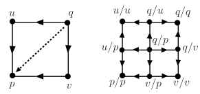
Figure 8: Orientations $o$ and $o^{*}$

In fact, ${\mit\Gamma}^{*}$ does not depend on the choice of an admissible orientation; see [10].

An edge joining $q/p$ and $q^{\prime}/p$ (resp. $q/p$ and $q/p^{\prime}$) is denoted by $qq^{\prime}/p$ (resp. $q/pp^{\prime}$). A function $h^{*}$ on $E_{{\mit\Gamma}^{*}}$ is defined as $h^{*}(qq^{\prime}/p):=h(qq^{\prime})/2$ and $h^{*}(q/pp^{\prime}):=h(pp^{\prime})/2$. Let $\boldsymbol{{\mit\Gamma}}^{*}:=({\mit\Gamma}^{*},o^{*},h^{*})$, which is called the $2$-subdivision of $\boldsymbol{{\mit\Gamma}}$.

Theorem 4.3.

For a modular complex $\boldsymbol{\mit\Gamma}$, the $2$-subdivision ${\boldsymbol{\mit\Gamma}}^{*}$ is also a modular complex.

This theorem will be proved in Section 4.3.2. Figure 9 illustrates the $2$-subdivision of $\boldsymbol{{\mit\Gamma}}$ in Figure 2.

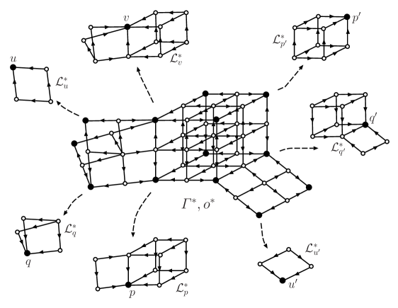
Figure 9: Construction of $\boldsymbol{{\mit\Gamma}}^{*}$ and neighborhood semilattices

By embedding $p\mapsto p/p$, we can regard $V_{{\mit\Gamma}}\subseteq V_{{\mit\Gamma}^{*}}$. The admissible orientation $o^{*}$ is oriented so that the vertices in $V_{{\mit\Gamma}}$ are all sinks. The partial order $\preceq_{o^{*}}$ on $V_{{\mit\Gamma}^{*}}$ induced by $o^{*}$ is denoted by $\preceq_{*}$, and $\sqsubseteq_{o^{*}}$ is also denoted by $\sqsubseteq_{*}$. In fact, one can show that two relations $\preceq_{*}$ and $\sqsubseteq_{*}$ are the same. Here we only note the following obvious relation:

(4.3) $$q/p\preceq_{*}q^{\prime}/p^{\prime}\Longleftrightarrow p^{\prime}\preceq p\preceq q\preceq q^{\prime}\quad(q/p,q^{\prime}/p^{\prime}\in{\cal B}(\boldsymbol{{\mit\Gamma}})).$$

For each vertex $p\in V_{{\mit\Gamma}}$, define the neighborhood semilattice ${\cal L}^{*}_{p}:={\cal L}_{p/p}^{+}(\boldsymbol{{\mit\Gamma}}^{*})$. By Theorems 4.2 and 4.3, we obtain:

Proposition 4.4.

Let $\boldsymbol{{\mit\Gamma}}$ be a modular complex. For each vertex $p$, the neighborhood semilattice ${\cal L}^{*}_{p}$ is a complemented modular semilattice with the minimum element $p$.

See Figure 9. Neighborhood semilattice ${\cal L}^{*}_{p}$ has more information about the local property of $p$ than ${\cal L}^{+}_{p}$ and ${\cal L}^{-}_{p}$ have.

Valuation of local semilattices.

A positive orbit-invariant function $h$ naturally gives valuation $v_{p}$ on ${\cal L}_{p}^{s}$ for $s\in\{-,+\}$, and valuation $v_{p}^{*}$ on ${\cal L}_{p}^{*}$ by

(4.4) $$v_{p}(q) := d_{{\mit\Gamma},h}(q,p)\quad(q\in{\cal L}_{p}^{s},s\in\{-,+\}),$$

$$v^{*}_{p}(v/u) := d_{{\mit\Gamma}^{*},h^{*}}(v/u,p/p)\quad(v/u\in{\cal L}_{p}^{*}).$$

See Lemma 2.14. In the sequel, semilattices ${\cal L}_{p}^{+}$, ${\cal L}_{p}^{-}$, and ${\cal L}_{p}^{*}$ are supposed to be endowed with these valuations.

Embedding of $\boldsymbol{{\mit\Gamma}}$ into $\boldsymbol{{\mit\Gamma}}^{*}$.

The distances on ${\mit\Gamma}$ and ${\mit\Gamma}^{*}$ are related as follows.

Proposition 4.5.

Let $\boldsymbol{{\mit\Gamma}}=({\mit\Gamma},o,h)$ be a modular complex, and $\boldsymbol{{\mit\Gamma}}^{*}$ the $2$-subdivision of $\boldsymbol{{\mit\Gamma}}$. Then we have

(4.5) $$d_{{\mit\Gamma}^{*},h^{*}}(q/p,q^{\prime}/p^{\prime})=\frac{d_{{\mit\Gamma},h}(p,p^{\prime})+d_{{\mit\Gamma},h}(q,q^{\prime})}{2}\quad(q/p,q^{\prime}/p^{\prime}\in{\cal B}(\boldsymbol{{\mit\Gamma}})=V_{{\mit\Gamma}^{*}}).$$

In particular, $(V_{\mit\Gamma},d_{{\mit\Gamma},h})$ is isometrically embedded into $(V_{{\mit\Gamma}^{*}},d_{{\mit\Gamma}^{*},h^{*}})$ by $p\mapsto p/p$.

This proposition will be proved in Section 4.3.2.

Product of modular complexes.

Suppose that we are given two modular complexes $\boldsymbol{{\mit\Gamma}}=({\mit\Gamma},o,h)$ and $\boldsymbol{{\mit\Gamma}}^{\prime}=({\mit\Gamma}^{\prime},o^{\prime},h^{\prime})$. Then the Cartesian product ${\mit\Gamma}\times{\mit\Gamma}^{\prime}$ is also modular. Furthermore, define the orientation $o\times o^{\prime}$ of ${\mit\Gamma}\times{\mit\Gamma}^{\prime}$ as: $(p,p^{\prime})\swarrow_{o\times o^{\prime}}(p,q^{\prime})$ if $p^{\prime}\swarrow_{o^{\prime}}q^{\prime}$ and $(p,p^{\prime})\swarrow_{o\times o^{\prime}}(q,p^{\prime})$ if $p\swarrow_{o}q$. Then $o\times o^{\prime}$ is an admissible orientation. Similarly define $h\times h^{\prime}$ by $(h\times h^{\prime})((p,p^{\prime})(q,p^{\prime})):=h(pq)$ and $(h\times h^{\prime})((p,p^{\prime})(p,q^{\prime})):=h^{\prime}(p^{\prime}q^{\prime})$, which is orbit-invariant in ${\mit\Gamma}\times{\mit\Gamma}^{\prime}$. Thus we obtain a new modular complex $\boldsymbol{{\mit\Gamma}}\times\boldsymbol{{\mit\Gamma}}^{\prime}:=({\mit\Gamma}\times{\mit\Gamma}^{\prime},o\times o^{\prime},h\times h^{\prime})$, which is called the product of $\boldsymbol{{\mit\Gamma}}$ and $\boldsymbol{{\mit\Gamma}}^{\prime}$.

Lemma 4.6.

$(p,p^{\prime})\sqsubseteq_{o\times o^{\prime}}(q,q^{\prime})$ if and only if $p\sqsubseteq_{o}q$ and $p^{\prime}\sqsubseteq_{o^{\prime}}q^{\prime}$.

Proof.

Since $[(p,p^{\prime}),(q,q^{\prime})]\simeq[p,q]\times[p^{\prime},q^{\prime}]$, $[(p,p^{\prime}),(q,q^{\prime})]$ is complemented modular if and only if both $[p,q]$ and $[p^{\prime},q^{\prime}]$ are complemented modular. Thus, by Proposition 4.1, we have the claim. ∎

In particular the correspondence ${\cal B}(\boldsymbol{{\mit\Gamma}}\times\boldsymbol{{\mit\Gamma}}^{\prime})\ni(q,q^{\prime})/(p,p^{\prime})\mapsto(q/p,q^{\prime}/p^{\prime})\in{\cal B}(\boldsymbol{{\mit\Gamma}})\times{\cal B}(\boldsymbol{{\mit\Gamma}}^{\prime})$ is bijective, and we can regard

$${\cal B}(\boldsymbol{{\mit\Gamma}}\times\boldsymbol{{\mit\Gamma}}^{\prime})={\cal B}(\boldsymbol{{\mit\Gamma}})\times{\cal B}(\boldsymbol{{\mit\Gamma}}^{\prime}).$$

Under this correspondence, the product operation and the 2-subdivision operation commute in the following sense.

Lemma 4.7.

• ${\cal L}^{s}_{(p,p^{\prime})}(\boldsymbol{{\mit\Gamma}}\times\boldsymbol{{\mit\Gamma}}^{\prime})={\cal L}^{s}_{p}(\boldsymbol{{\mit\Gamma}})\times{\cal L}^{s}_{p^{\prime}}(\boldsymbol{{\mit\Gamma}}^{\prime})$ for $s\in\{-,+\}$.

• $(\boldsymbol{{\mit\Gamma}}\times\boldsymbol{{\mit\Gamma}}^{\prime})^{*}=\boldsymbol{{\mit\Gamma}}^{*}\times{\boldsymbol{{\mit\Gamma}}^{\prime}}^{*}$.

• ${\cal L}^{*}_{(p,p^{\prime})}(\boldsymbol{{\mit\Gamma}}\times\boldsymbol{{\mit\Gamma}}^{\prime})={\cal L}^{*}_{p}(\boldsymbol{{\mit\Gamma}})\times{\cal L}^{*}_{p^{\prime}}(\boldsymbol{{\mit\Gamma}}^{\prime})$.

Proof.

(1) follows from the previous lemma. (2) follows from the fact that $(q,q^{\prime})/(p,p^{\prime})$ and $(v,v^{\prime})/(u,u^{\prime})$ have an edge in $({\mit\Gamma}\times{\mit\Gamma}^{\prime})^{*}$ if and only if $d_{{\mit\Gamma}}(q,v)+d_{{\mit\Gamma}^{\prime}}(q^{\prime},v^{\prime})+d_{{\mit\Gamma}}(p,u)+d_{{\mit\Gamma}^{\prime}}(p^{\prime},u^{\prime})=1$, which is equivalent to the condition that $(q/p,q^{\prime}/p^{\prime})$ and $(v/u,v^{\prime}/u^{\prime})$ have an edge in ${\mit\Gamma}^{*}\times{\mit\Gamma}^{\prime*}$. (3) follows from (2). ∎

4.2 L-convex function on modular complex

We are ready to introduce the concept of an L-convex function on a modular complex $\boldsymbol{{\mit\Gamma}}=({\mit\Gamma},o,h)$. Consider the $2$-subdivision $\boldsymbol{{\mit\Gamma}}^{*}$ of $\boldsymbol{{\mit\Gamma}}$. For a function $g:V_{{\mit\Gamma}}\to{\bf R}$, define $\overline{g}:V_{{\mit\Gamma}^{*}}\to{\bf R}$ by

(4.6) $$\overline{g}(q/p):=\frac{g(p)+g(q)}{2}\quad(q/p\in{\cal B}(\boldsymbol{{\mit\Gamma}})=V_{{\mit\Gamma}^{*}}).$$

This is the restriction of the Lovász extension of $g$; see the introduction for the Lovász extension. By restricting $\overline{g}$ to neighborhood semilattices, we obtain functions on (complemented) modular semilattices ${\cal L}^{*}_{p}$ for each vertex $p$.

An L-convex function on $\boldsymbol{{\mit\Gamma}}$ is a function $g:V_{{\mit\Gamma}}\to{\bf R}$ such that for each vertex $p\in V_{{\mit\Gamma}}$ the restriction of $\overline{g}$ to ${\cal L}^{*}_{p}$ is submodular on ${\cal L}^{*}_{p}$ (with respect to the valuation $v^{*}_{p}$). Corresponding to Theorem 3.6, the distance function $d_{{\mit\Gamma},h}$ is L-convex on $\boldsymbol{{\mit\Gamma}}\times\boldsymbol{{\mit\Gamma}}$, which is one of the most important properties for our application to 0-extension problem.

Theorem 4.8.

For a modular complex $\boldsymbol{{\mit\Gamma}}=({\mit\Gamma},o,h)$, the distance function $d_{{\mit\Gamma},h}$ is an L-convex function on $\boldsymbol{{\mit\Gamma}}\times\boldsymbol{{\mit\Gamma}}$.

The proof of this theorem is given in Section 4.3.3. Corresponding to Lemma 3.7, we obtain:

Lemma 4.9.

Let $\boldsymbol{{\mit\Gamma}},\boldsymbol{{\mit\Gamma}}^{\prime},\boldsymbol{{\mit\Lambda}}$, and $\boldsymbol{{\mit\Lambda}}^{\prime}$ be modular complexes, and let $g$ and $g^{\prime}$ be L-convex functions on $\boldsymbol{{\mit\Gamma}}$.

• For $b\in{\bf R}$ and $c,c^{\prime}\in{\bf R}_{+}$, $b+cg+c^{\prime}g^{\prime}$ is an L-convex function on $\boldsymbol{{\mit\Gamma}}$.

• A function $\tilde{g}$ defined by

  $$\tilde{g}(p,p^{\prime}):=g(p)\quad((p,p^{\prime})\in V_{{\mit\Gamma}\times{\mit\Gamma}^{\prime}})$$

  is an L-convex function on ${\boldsymbol{{\mit\Gamma}}}\times{\boldsymbol{{\mit\Gamma}}}^{\prime}$.

• Suppose that ${\boldsymbol{{\mit\Gamma}}}={\boldsymbol{{\mit\Lambda}}}\times{\boldsymbol{{\mit\Lambda}}}^{\prime}$. For $p^{\prime}\in V_{{\mit\Lambda}^{\prime}}$, a function $g_{p^{\prime}}$ defined by

  $$g_{p^{\prime}}(p):=g(p,p^{\prime})\quad(p\in V_{{\mit\Lambda}})$$

  is an L-convex function on $\boldsymbol{{\mit\Lambda}}$.

Proof.

(1) follows from Lemma 3.7 (1).

(2). $\overline{(\tilde{g})}(q/p,q^{\prime}/p^{\prime})=\{\tilde{g}(p,p^{\prime})+\tilde{g}(q,q^{\prime})\}/2=\{g(p)+g(q)\}/2=\overline{g}(q/p)$. Therefore, by Lemma 3.7 (2), function $(q/p,q^{\prime}/p^{\prime})\mapsto\overline{g}(q/p)$ is submodular on ${\cal L}^{*}_{p}(\boldsymbol{{\mit\Gamma}})\times{\cal L}^{*}_{p^{\prime}}(\boldsymbol{{\mit\Gamma}}^{\prime})={\cal L}^{*}_{(p,p^{\prime})}(\boldsymbol{{\mit\Gamma}}\times\boldsymbol{{\mit\Gamma}}^{\prime})$.

(3). $\overline{g_{p^{\prime}}}(q/p)=\{g(p,p^{\prime})+g(q,p^{\prime})\}/2=\overline{g}(q/p,p^{\prime}/p^{\prime})$. Since $\overline{g}$ is submodular on ${\cal L}_{p}^{*}(\boldsymbol{{\mit\Lambda}})\times{\cal L}_{p^{\prime}}^{*}(\boldsymbol{{\mit\Lambda}}^{\prime})$, by Lemma 3.7 (3), $\overline{g_{p^{\prime}}}$ is submodular on ${\cal L}_{p}^{*}(\boldsymbol{{\mit\Lambda}})$. ∎

The restrictions of an L-convex function to ${\cal L}_{p}^{+}$ and to ${\cal L}_{p}^{-}$ are submodular.

Lemma 4.10.

An L-convex function $g$ on $\boldsymbol{{\mit\Gamma}}$ is submodular on ${\cal L}^{+}_{p}$ and on ${\cal L}_{p}^{-}$ for each vertex $p$.

Proof.

Consider the set ${\cal L}_{p}^{*+}$ of elements in ${\cal L}_{p}^{*}$ of the form $q/p$. By Proposition 4.5, any vertex in any shortest path between $q/p$ and $q^{\prime}/p$ is of the form $u/p$. Hence ${\cal L}_{p}^{*+}$ is convex in ${\mit\Gamma}$ and in ${\cal L}_{p}^{*}$. By Lemma 3.7 (4), $\overline{g}$ is submodular on ${\cal L}_{p}^{*+}$. Obviously ${\cal L}_{p}^{*+}$ is isomorphic to ${\cal L}_{p}^{+}$ by $q/p\mapsto q$. By using relation $g(q)=2\overline{g}(q/p)-g(p)$ $(q\in{\cal L}^{+}_{p})$, we see the submodularity of $g$ on ${\cal L}^{+}_{p}$. ∎

L-optimality criterion.

Consider minimization of L-convex functions on a modular complex $\boldsymbol{{\mit\Gamma}}$. There is an optimality criterion that extends the L-optimality criterion of L^♮-convex function in discrete convex analysis; see [47, Theorem 7.14].

Theorem 4.11 (L-optimality criterion).

Let $g$ be an L-convex function on a modular complex $\boldsymbol{{\mit\Gamma}}$. For a vertex $p\in V_{\mit\Gamma}$, the following conditions are equivalent:

• $g(p)\leq g(q)$ holds for every $q\in V_{{\mit\Gamma}}$.

• $g(p)\leq g(q)$ holds for every $q\in V_{{\mit\Gamma}}$ with $p\sqsubseteq q$ or $q\sqsubseteq p$. That is

  $$g(p)=\min\{g(q)\mid q\in{\cal L}_{p}^{+}\}=\min\{g(q)\mid q\in{\cal L}_{p}^{-}\}.$$

We prove this theorem in Section 4.3.4. The condition (2) implies that $g$ can be minimized by tracing the 1-skeleton graph of ${\mit\Delta}(\boldsymbol{{\mit\Gamma}})$. By Lemma 4.10, checking the condition ($2$) reduces to the submodular function minimization on modular semilattices, analogous to the case of L^♮-convex function in discrete convex analysis [47, Section 10.3].

Suppose that $\boldsymbol{{\mit\Gamma}}$ is the product of modular complexes $\boldsymbol{{\mit\Gamma}}_{i}$ for $i=1,2,\ldots,n$. Again we say nothing about the complexity of the minimization under the oracle model. So we consider the VSCP situation. Recall Section 2.1. By an L-convex constraint on $\boldsymbol{{\mit\Gamma}}$ we mean an L-convex function $g$ on $\boldsymbol{{\mit\Gamma}}_{i_{1}}\times\boldsymbol{{\mit\Gamma}}_{i_{2}}\times\cdots\times\boldsymbol{{\mit\Gamma}}_{i_{k}}$ for some $i_{1}<i_{2}<\cdots<i_{k}$. By Lemma 4.9, the sum of L-convex constraints ${\cal G}$ is an L-convex function on $\boldsymbol{{\mit\Gamma}}$. By L-optimality criterion, the optimality check of given vertex $p$ reduces to the minimization of the sum of submodular constraints over modular semilattices ${\cal L}^{s}_{p}(\boldsymbol{{\mit\Gamma}})={\cal L}^{s}_{p_{1}}\times{\cal L}^{s}_{p_{2}}\times\cdots\times{\cal L}^{s}_{p_{n}}$ for $s\in\{-,+\}$. By Theorem 3.9, we obtain:

Theorem 4.12.

Let $\boldsymbol{{\mit\Gamma}}$ be the product of modular complexes $\boldsymbol{{\mit\Gamma}}_{i}$ $(i=1,2,\ldots,n)$, and let ${\cal G}$ be a set of L-convex constraints on $\boldsymbol{{\mit\Gamma}}$. Define $g:V_{{\mit\Gamma}}\to{\bf R}$ by

$$g(p):=\sum_{h\in{\cal G}}h(p_{I_{h}})\quad(p=(p_{1},p_{2},\ldots,p_{n})\in V_{{\mit\Gamma}}).$$

For a given vertex $p$, there exists an algorithm, in time polynomial in $n$ and $|{\cal G}|L^{K}$, to find $q\in{\cal L}^{-}_{p}\cup{\cal L}^{+}_{p}$ with $g(q)<g(p)$ or conclude that $p$ is a global minimizer of $g$, where $L:=\max_{1\leq i\leq n,s\in\{+,-\}}|{\cal L}_{p_{i}}^{s}|$ and $K:=\max_{g\in{\cal G}}k_{g}$.

Steepest descent algorithm.

Theorem 4.11, Lemma 4.10, and Theorem 3.9 naturally lead us to a descent algorithm for L-convex functions on modular complexes, analogous to the steepest descent algorithm for L-convex function minimization in discrete convex analysis.

Starting from an arbitrary point $p$, each descent step is to find, for $s\in\{-,+\}$, an optimal solution $q^{s}$ of the problem:
$(4.7)$    Minimize $g(q)$ over $q\in{\cal L}_{p}^{s}$.
As mentioned already, this is a submodular function minimization. If $g(p)=g(q^{+})=g(q^{-})$, then $p$ is optimal. Otherwise, take $s\in\{-,+\}$ with $g(q^{s})=\min\{g(q^{-}),g(q^{+})\}(<g(p))$, let $p:=q^{s}$ (steepest direction), and repeat the descent step. After a finite number of descent steps, we can obtain an optimal solution (a minimizer of $g$).

In the case where $f$ is an L^♮-convex function on a box subset $B$ of ${\bf Z}^{n}$, Murota [46] proved that, by appropriate choices of steepest directions, the number of the descent steps is bounded by $l_{1}$-diameter of $B$; later Kolmogorov and Shioura [40] improved this bound. We do not know whether a similar upper bound exists for L-convex function minimizations on general modular complexes. This issue will be studied in [26].

4.3 Proofs

4.3.1 Proof of Proposition 4.1 and Theorem 4.2

We can assume that $h$ is the uniform unit edge weight, and $d_{{\mit\Gamma},h}=d_{{\mit\Gamma}}$ is denoted by $d$. A path $(p_{0},p_{1},p_{2},\ldots,p_{k})$ is said to be ascending if $p_{i}\swarrow p_{i+1}$ for $i=0,\ldots,k-1$.

Lemma 4.13.

For $p,q\in V_{\mit\Gamma}$ with $p\preceq q$, a $(p,q)$-path $P$ is shortest if and only if $P$ is an ascending path from $p$ to $q$. In particular, $I(p,q)=[p,q]$, any maximal chain in $[p,q]$ has the same length, and the rank $r$ of $[p,q]$ is given by $r(a)=d(a,p)$.

Proof.

Suppose $p\preceq q$. Take an ascending path $P=(p=p_{0},p_{1},p_{2},\ldots,p_{k}=q)$. We use the induction on length $k$; the statement for $k=1$ is obvious.

(If part). We show $d(p,q)=k$. Suppose for contradiction that $d(p,q)<k$. By induction and bipartiteness, we have $d(p,p_{k})=d(p,p_{k-1})-1$ and $d(p,p_{k-1})=k-1$. By the quadrangle condition (Lemma 2.3 (2)) for $p_{k-1},p_{k},p_{k-2},p$, there is a common neighbor $q^{*}$ of $p_{k},p_{k-2}$ with $d(p,q^{*})=d(p,p_{k-1})-2=k-3$. Consider the 4-cycle of $p_{k-1},p_{k},q^{*},p_{k-2}$. By orientability $p_{k-2}\swarrow q^{*}$ must hold. Hence we obtain an ascending path $(p=p_{0},p_{1},\ldots,p_{k-2},q^{*})$ of length $k-1$ with $d(p,q^{*})=k-3$. A contradiction.

(Only if part). Take any shortest path $Q=(p=q_{0},q_{1},q_{2},\ldots,q_{k^{\prime}}=q)$ between $p$ and $q$. We show that $Q$ is ascending. By the if part, necessarily $k^{\prime}=k$. It suffices to show that $p\preceq q_{k-1}\swarrow q$; by induction $(p=q_{0},q_{1},q_{2},\ldots,q_{k-1})$ is ascending, and hence $Q$ is ascending. We can assume that $p_{k-1}\neq q_{k-1}$. By the quadrangle condition for $q,p_{k-1},q_{k-1},p$, there is a common neighbor $q^{*}$ of $p_{k-1},q_{k-1}$ with $d(q^{*},p)=d(q,p)-2$. Then $q^{*}\in I(p,p_{k-1})=[p,p_{k-1}]$ (by induction). This means $p\preceq q^{*}\swarrow p_{k-1}$, which in turn implies $q^{*}\swarrow q_{k-1}\swarrow q$ by the orientation of 4-cycle $(p_{k-1},q,q_{k-1},q^{*})$. Thus $p\preceq q_{k-1}\swarrow q$, as required. ∎

Let $(p)^{\uparrow}$ and $(p)^{\downarrow}$ denote the principal filter $\{q\in V_{{\mit\Gamma}}\mid q\succeq p\}$ and the principal ideal $\{q\in V_{{\mit\Gamma}}\mid q\preceq p\}$ of $p$, respectively.

Lemma 4.14.

For $a,b\in(p)^{\uparrow}$, there uniquely exists a median $m$ of $p,a,b$, which coincides with $a\wedge b$. Similarly, for $a,b\in(p)^{\downarrow}$ there uniquely exists a median $m$ of $q,a,b$, which coincides with $a\vee b$. Both $(p)^{\uparrow}$ and $(p)^{\downarrow}$ are convex, and modular semilattices.

Proof.

It suffices to prove the claim for $(p)^{\uparrow}$. Suppose that $a,b,p$ have two distinct medians $c,c^{\prime}$. Take a median $m$ of $c,c^{\prime},p$. Let $k:=d(c,m)=d(c^{\prime},m)>0$. We can take an ascending path $(m=m_{0},m_{1},\ldots,m_{k}=c)$ from $m$ to $c$, and also can take a neighbor $m^{\prime}$ of $m$ with $d(m,c^{\prime})=1+d(m^{\prime},c^{\prime})$; necessarily $m\swarrow m^{\prime}$. By the quadrangle condition for $m,m_{1},m^{\prime},a$, there is a common neighbor $m_{1}^{\prime}$ of $m_{1},m^{\prime}$ such that $d(a,m^{\prime}_{1})=d(a,m)-2$. Also by the quadrangle condition for $m,m_{1},m^{\prime},b$ there is a common neighbor $m_{1}^{\prime\prime}$ of $m_{1},m^{\prime}$ such that $d(b,m_{1}^{\prime\prime})=d(b,m)-2$. By $m_{1}\searrow m\swarrow m^{\prime}$ and the orientability, we have $m_{1}\swarrow m^{\prime}_{1}\searrow m^{\prime}$ and $m_{1}\swarrow m^{\prime\prime}_{1}\searrow m^{\prime}$. Hence $m^{\prime}_{1}=m^{\prime\prime}_{1}$ must hold. Similarly, by the quadrangle condition for $m_{1},m_{2},m_{1}^{\prime},a$ and for $m_{1},m_{2},m_{1}^{\prime},b$, we can find a common neighbor $m_{2}^{\prime}$ of $m_{2},m^{\prime}_{1}$ such that $d(m_{2},a)=d(m_{2}^{\prime},a)+1$ and $d(m_{2},b)=d(m^{\prime}_{2},b)+1$. Necessarily $m_{2}\preceq m_{2}^{\prime}\preceq a,b$. Repeat this process to obtain a neighbor $m^{\prime}_{k}$ of $m_{k}(=c)$ such that $d(c,a)=d(m^{\prime}_{k},a)+1$ and $d(c,b)=d(m^{\prime}_{k},b)+1$. This implies that $d(a,b)\leq d(a,m^{\prime}_{k})+d(m^{\prime}_{k},b)=d(a,c)+d(c,b)-2=d(a,b)-2$; a contradiction.

We show $m=a\wedge b$ in the poset $(p)^{\uparrow}$. Indeed, take an arbitrary $p^{\prime}\in(p)^{\uparrow}$ with $a\succeq p^{\prime}\preceq b$. Consider a median $m^{\prime}$ of $a,b,p^{\prime}$. Since there is an ascending path from $p$ to $m^{\prime}$ using $p^{\prime}$, $m^{\prime}$ is also a median of $a,b,p$, and $m^{\prime}=m$ by the uniqueness. Hence $p^{\prime}\preceq m$.

We next show the convexity of $(p)^{\uparrow}$ by verifying (3) in Lemma 2.9. Clearly the subgraph of ${\mit\Gamma}$ induced by $(p)^{\uparrow}$ is connected. Take $a,b\in(p)^{\uparrow}$ with $d(a,b)=2$. We show that $I(a,b)\subseteq(p)^{\uparrow}$. From Lemma 4.13, this is obvious when $a\preceq b$ or $b\preceq a$. Thus we may assume $a\not\preceq b$ and $b\not\preceq a$. Consider $a\wedge b$ in $(p)^{\uparrow}$ (the existence of $a\wedge b$ is guaranteed as above). By $d(a,b)=2$, $a$ and $b$ cover $a\wedge b$. By the admissibility of the orientation $o$, if $a$ and $b$ have another common neighbor $c\neq a\wedge b$, then $c$ covers $a$ and $b$, i.e., $c=a\vee b\in(p)^{\uparrow}$. Hence $I(a,b)\subseteq(p)^{\uparrow}$, and $(p)^{\uparrow}$ is convex.

For arbitrary $a,b\in(p)^{\uparrow}$, every maximal common lower bound $m^{\prime}$ of $a,b$ (not necessarily in $(p)^{\uparrow}$) belong to $I(a,b)$; consider a median $m^{\prime},a,b$, which is equal to $m^{\prime}$ by the above argument. By the convexity, $m^{\prime}$ belongs to $(p)^{\uparrow}$, and is equal to $a\wedge b$ in $(p)^{\uparrow}$. This means that $a,b$ have the meet in the poset $(V_{{\mit\Gamma}},\preceq)$.

Now $(p)^{\uparrow}$ is a semilattice, and convex in ${\mit\Gamma}$. The covering graph of $(p)^{\uparrow}$ is equal to the subgraph ${\mit\Gamma}[(p)^{\uparrow}]$ induced by $(p)^{\uparrow}$, which is modular (by convexity). By Theorem 2.12, $(p)^{\uparrow}$ is a modular semilattice. ∎

Proof of Proposition 4.1.

(1). Notice that the convexity is closed under the intersection. By $[p,q]=(p)^{\uparrow}\cap(q)^{\downarrow}$ and by the previous lemma, we have the convexity of $[p,q]$. Also $[p,q]$ is an interval of a modular semilattice, and hence a modular lattice.

(2). If $(p,q)$ is Boolean, then $q$ is the join of atoms in $[p,q]$, and $[p,q]$ is a complemented modular lattice (Theorem 2.11). Conversely, if $[p,q]$ is a complemented modular lattice, then there is a Boolean sublattice of full rank (generated by a base), and $(p,q)$ is Boolean.

We can check whether a pair $(p,q)$ is Boolean by the following procedure. First construct the partial order $\preceq$, and the poset $(V_{{\mit\Gamma}},\preceq)$. If $p\not\preceq q$, then $(p,q)$ is not Boolean. Suppose $p\preceq q$. Construct (or enumerate) $[p,q]$. For each $u\in[p,q]$, check the existence of an element (complement) $v\in[p,q]$ with $u\wedge v=p$ and $u\vee v=q$. If every element has a complement, then $[p,q]$ is complemented modular, and $(p,q)$ is Boolean. Otherwise, $(p,q)$ is not Boolean. This procedure can be done in time polynomial in $|V_{{\mit\Gamma}}|$. $\Box$

Proof of Theorem 4.2.

It suffices to consider only ${\cal L}_{p}^{+}$. The statement that ${\cal L}_{p}^{+}$ is a semilattice immediately follows from Lemma 4.14 and (4.1). Next we show the convexity. In view of Lemma 2.9, take $a,b\in{\cal L}^{+}_{p}$ with $d(a,b)=2$, and take any common neighbor $c$ of $a,b$. We show $c\in{\cal L}^{+}_{p}$. This is obvious if $a\swarrow c\swarrow b$ or $b\swarrow c\swarrow a$. Also, if $a\searrow c\swarrow b$, then $c=a\wedge b\in{\cal L}^{+}_{p}$ (if $c\neq a\wedge b$, then 4-cycle $(a,c,b,a\wedge b)$ violates the admissibility of the orientation $o$).

So suppose that $a\swarrow c\searrow b$. By Lemma 4.13, both $[p,a]$ and $[p,b]$ belong to $[p,c]$. In particular, $c$ is the join of $a$ and $b$ in $[p,c]$. Here $a$ is the join of atoms in $[p,a]$ and $b$ is the join of atoms in $[p,b]$. This means that $c$ is the join of atoms in $[p,c]$. Hence modular lattice $[p,c]$ is complemented (Theorem 2.11), and hence $(p,c)$ is Boolean.

The subgraph of ${\mit\Gamma}$ induced by any convex set is again a modular graph. Therefore the covering graph of ${\cal L}^{+}_{p}$ is modular. By Theorem 2.12, ${\cal L}^{+}_{p}$ is a modular semilattice. In particular, each $[p,q]$ for each $q\in{\cal L}^{+}_{p}$ is a complemented modular lattice, and ${\cal L}^{+}_{p}$ is a complemented modular semilattice. $\Box$

4.3.2 Proof of Theorem 4.3 and Proposition 4.5

We start with preliminary results. By Proposition 4.1, interval $[p,q]$ is a modular lattice, and is convex in ${\mit\Gamma}$. So we can consider the projection $\mathop{\rm Pr}_{[p,q]}:V_{{\mit\Gamma}}\to[p,q]$ (see Section 2.2.2).

Lemma 4.15.

For $p,q,p^{\prime},q^{\prime}\in V_{{\mit\Gamma}}$ with $p\preceq q$ and $p^{\prime}\preceq q^{\prime}$, let $u,v,u^{\prime},v^{\prime}$ be defined by

(4.8) $$u:={\rm Pr}_{[p,q]}(p^{\prime}),\ v:={\rm Pr}_{[p,q]}(q^{\prime}),u^{\prime}:={\rm Pr}_{[p^{\prime},q^{\prime}]}(p),\ v^{\prime}:={\rm Pr}_{[p^{\prime},q^{\prime}]}(q).$$

Then we have:

• $u\preceq v$, $u^{\prime}\preceq v^{\prime}$, $\mathop{\rm Pr}_{[p^{\prime},q^{\prime}]}([p,q])=[u^{\prime},v^{\prime}]$, and $\mathop{\rm Pr}_{[p,q]}([p^{\prime},q^{\prime}])=[u,v]$.

• $[u,v]$ is isomorphic to $[u^{\prime},v^{\prime}]$ by map $w\mapsto\mathop{\rm Pr}_{[p^{\prime},q^{\prime}]}(w)$. In particular, $p\sqsubseteq q$ implies $u^{\prime}\sqsubseteq v^{\prime}$.

Proof.

The image of a convex set by the projection is again convex (Theorem 2.8), and a convex set in a modular lattice is exactly an interval (Lemma 2.16 (2)). Hence $\mathop{\rm Pr}_{[p^{\prime},q^{\prime}]}([p,q])$ is equal to a subinterval $[a^{\prime},b^{\prime}]$ of $[p^{\prime},q^{\prime}]$, and $\mathop{\rm Pr}_{[p,q]}([p^{\prime},q^{\prime}])$ is equal to a subinterval $[a,b]$ of $[p,q]$. By Theorem 2.8, $\Pr_{[p,q]}$ is an isometry between $[a,b]$ and $[a^{\prime},b^{\prime}]$, and consequently this induces a graph isomorphism between the subgraphs induced by $[a,b]$ and $[a^{\prime},b^{\prime}]$. By Lemma 2.5, for $g,h\in[a,b]$, if $g\swarrow h$ then $\mathop{\rm Pr}_{[p^{\prime},q^{\prime}]}(g)\swarrow\mathop{\rm Pr}_{[p^{\prime},q^{\prime}]}(h)$. Therefore, a poset $[a,b]$ is isomorphic to $[a^{\prime},b^{\prime}]$ by $\Pr_{[p^{\prime},q^{\prime}]}$. Necessarily $\mathop{\rm Pr}_{[p,q]}(a^{\prime})=a$. Notice that $a$ is the gate of $p$ at $[a,b]$ (by Lemma 4.13). By Theorem 2.8 (3), $a=\mathop{\rm Pr}_{[a,b]}(p)=\mathop{\rm Pr}_{[p,q]}\circ\mathop{\rm Pr}_{[p^{\prime},q^{\prime}]}(p)=\mathop{\rm Pr}_{[p,q]}(u^{\prime})$. Then $\mathop{\rm Pr}_{[p,q]}(u^{\prime})=a=\mathop{\rm Pr}_{[p,q]}(a^{\prime})$ implies $a^{\prime}=u^{\prime}$ (by Theorem 2.8 (1)). Similarly $b^{\prime}=v^{\prime}$, $a=u$, and $b=v$. Thus we obtain (1) and (2). ∎

We use the same notation $d$ for $d_{{\mit\Gamma}}$ and $d_{{\mit\Gamma}^{*},1/2}$ (since they can be distinguished by the arguments).

Lemma 4.16.

$\displaystyle d(q/p,q^{\prime}/p^{\prime})=\frac{d(p,p^{\prime})+d(q,q^{\prime})}{2}$ for $q/p,q^{\prime}/p^{\prime}\in V_{{\mit\Gamma}^{*}}$.

Proof.

Take a path $P=(q/p=q_{0}/p_{0},q_{1}/p_{1},\ldots,q_{k}/p_{k}=q^{\prime}/p^{\prime})$ between $q/p$ and $q^{\prime}/p^{\prime}$ in ${\mit\Gamma}^{*}$. The length of $P$ is equal to $\sum_{i=0}^{k-1}(d(q_{i},q_{i+1})+d(p_{i},p_{i+1}))/2\geq(d(q,q^{\prime})+d(p,p^{\prime}))/2$; hence $(\geq)$ holds.

We show the equality by the induction on $d(p,p^{\prime})+d(q,q^{\prime})$. Define $u,v,u^{\prime},v^{\prime}$ by (4.8). Then $d(p,p^{\prime})=d(p,u)+d(u,u^{\prime})+d(u^{\prime},p^{\prime})$ and $d(q,q^{\prime})=d(q,v)+d(v,v^{\prime})+d(v^{\prime},q^{\prime})$ hold. Suppose $p\prec u$. Take an atom $a$ of $[p,u]$. Then $(a,q)$ is Boolean by (4.1), and $q/a$ is adjacent to $q/p$ in ${\mit\Gamma}^{*}$. Also $d(a,u)=d(p,u)-1$ (Lemma 4.13), implying $d(a,p^{\prime})=d(p,p^{\prime})-1$. By induction, $d(q/a,q^{\prime}/p^{\prime})=(d(a,p^{\prime})+d(q,q^{\prime}))/2$, and hence $d(q/p,q^{\prime}/p^{\prime})\leq(d(a,p^{\prime})+d(q,q^{\prime}))/2+1/2=(d(p,p^{\prime})+d(q,q^{\prime}))/2$, as required.

Consequently we can assume $(p,q,p^{\prime},q^{\prime})=(u,v,u^{\prime},v^{\prime})$. In particular, $d(p,q)=d(p^{\prime},q^{\prime})$, $d(p,p^{\prime})=d(q,q^{\prime})$, and $d(p,q^{\prime})=d(p,q)+d(q,q^{\prime})=d(q,p^{\prime})$ must hold. Take a neighbor $a$ of $p$ in $I(p,p^{\prime})$; then $a\not\in[p,q]$. Take a median $b$ of $q,a,q^{\prime}$. Then $b$ must be a neighbor of $q$ and satisfies $d(p,q)=d(a,b)=d(p,b)-1=d(a,q)-1$. If $q\swarrow b$, then $p\swarrow a\preceq b$ (Lemma 4.13), and the join $q\vee a$ in $[p,b]$ is equal to $b$; this means that $[p,b]$ is a complemented modular lattice, $(p,b)$ is Boolean, and $b/p$ is adjacent to $q/p$. Applying the induction to $b/p$ and $q^{\prime}/p^{\prime}$, we obtain the equality ($=$). Similarly, if $b\swarrow q$, then $(a,q)$ is Boolean and apply the induction to $q/a$ and $q^{\prime}/p^{\prime}$. ∎

Proof of Theorem 4.3.

Any 4-cycle in ${\mit\Gamma}^{*}$ is represented as $(q/p,q^{\prime}/p,q^{\prime}/p^{\prime},q/p^{\prime})$ for some edges $pp^{\prime},qq^{\prime}$ in ${\mit\Gamma}$, or $(x/p,y/p,z/p,w/p)$ or $(p/x,p/y,p/z,p/w)$ for 4-cycle $(x,y,z,w)$ and vertex $p$ in ${\mit\Gamma}$. This immediately implies that $o^{*}$ is an admissible orientation and $h^{*}$ is orbit-invariant.

To show that ${\mit\Gamma}^{*}$ is modular, we are going to verify that ${\mit\Gamma}^{*}$ satisfies the two conditions of Lemma 2.3. If $q/p$ and $q^{\prime}/p^{\prime}$ are joined by an edge, then $d_{{\mit\Gamma}}(p,q)$ and $d_{{\mit\Gamma}}(p^{\prime},q^{\prime})$ have different parity. This implies that ${\mit\Gamma}^{*}$ is bipartite.

We next verify the quadrangle condition (Lemma 2.3 (2)). Take boolean pairs $q/p$ and $q^{\prime}/p^{\prime}$. Suppose further that we are given two neighbors $q_{1}/p_{1}$ and $q_{2}/p_{2}$ of $q/p$ with $d(q/p,q^{\prime}/p^{\prime})=1/2+d(q_{1}/p_{1},q^{\prime}/p^{\prime})=1/2+d(q_{2}/p_{2},q^{\prime}/p^{\prime})$. Our goal is to show the existence of a common neighbor $q^{*}/p^{*}$ of $q_{1}/p_{1},q_{2}/p_{2}$ with $d(q/p,q^{\prime}/p^{\prime})=1+d(q^{*}/p^{*},q^{\prime}/p^{\prime})$.

It suffices to consider the following three cases:

• $p_{1}=p=p_{2}$.

• $p_{1}=p$, $q_{1}\swarrow q$, and $q_{2}=q$.

• $p_{1}\swarrow p=p_{2}$ and $q_{1}=q\swarrow q_{2}$.

Case (i). By Lemma 4.16, we have $d(q,q^{\prime})=1+d(q_{i},q^{\prime})$ for $i=1,2$. By Lemma 2.3 (2) for ${\mit\Gamma}$, there is a common neighbor $q^{*}$ of $q_{1},q_{2}$ with $d(q,q^{\prime})=2+d(q^{*},q^{\prime})$. Here $p\sqsubseteq q_{i}$ $(i=1,2)$, and hence $q_{i}\in{\cal L}^{+}_{p}$. By the convexity of ${\cal L}^{+}_{p}$ (Theorem 4.2), we have $q^{*}\in{\cal L}^{+}_{p}$, implying $p\sqsubseteq q^{*}$. Again, by Lemma 4.16, we have $d(q/p,q^{\prime}/p^{\prime})=1+d(q^{*}/p,q^{\prime}/p^{\prime})$, as required.

Case (ii). We show $p_{2}\sqsubseteq q_{1}$, which implies that $q_{1}/p_{2}$ is a required common neighbor (by Lemma 4.16). If $p_{2}\swarrow p$, then $p_{2}\sqsubseteq q$ and $p_{2}\swarrow p\preceq q_{1}\swarrow q$ imply $p_{2}\sqsubseteq q_{1}$ (by (4.1)). Suppose $p\swarrow p_{2}$. By Lemma 4.15, $\mathop{\rm Pr}_{[p,q]}([p^{\prime},q^{\prime}])$ is equal to interval $[a,b]$ for $a=\mathop{\rm Pr}_{[p,q]}(p^{\prime})$ and $b=\mathop{\rm Pr}_{[p,q]}(q^{\prime})$. Then $d(p_{2},p^{\prime})=d(p,p^{\prime})-1$ implies $p_{2}\preceq a$. Similarly $b\preceq q_{1}$. Thus $p\preceq p_{2}\preceq a\preceq b\preceq q_{1}\preceq q$ and $p\sqsubseteq q$ imply $p_{2}\sqsubseteq q_{1}$ (by (4.1)), as required.

Case (iii). We show $p_{1}\sqsubseteq q_{2}$; then $q_{2}/p_{1}$ is a common neighbor as required. We use the induction on $d(p_{1},q_{2})$; in the case of $d(p_{1},q_{2})=2$ the subsequent argument shows that $I(p_{1},q_{2})=[p_{1},q_{2}]$ contains an element different from $p_{1},q_{2},p$, and hence $(p_{1},q_{2})$ is Boolean. Since $[p_{1},q_{2}]$ is a convex set, we can consider $\mathop{\rm Pr}_{[p_{1},q_{2}]}([p^{\prime},q^{\prime}])$, which is equal to $[u,v]$ for $u:=\mathop{\rm Pr}_{[p_{1},q_{2}]}(p^{\prime})$, $v:=\mathop{\rm Pr}_{[p_{1},q_{2}]}(q^{\prime})$ (Lemma 4.15). Then necessarily $p\not\preceq u$; otherwise $d(p_{1},p^{\prime})=d(p_{1},u)+d(u,p^{\prime})=1+d(p,u)+d(u,p^{\prime})=1+d(p,p^{\prime})$, contradicting the first assumption $d(p_{1},p^{\prime})=d(p,p^{\prime})-1$.

Suppose $p_{1}\neq u$. Take an atom $a\in[p_{1},u]$. If $a\not\preceq q$, then $q_{2}$ is equal to the join $a\vee q$, and consequently the join of atoms in $[p_{1},q_{2}]$. Thus $[p_{1},q_{2}]$ is complemented, and $p_{1}\sqsubseteq q_{2}$ (Proposition 4.1). Suppose that $a\preceq q$. Consider the join $a\vee p$ in $[p_{1},q_{2}]$, which belongs to $[p,q]$. Then $d(a\vee p,p^{\prime})=d(a\vee p,u)+d(u,p^{\prime})=1+d(a,u)+d(u,p^{\prime})=1+d(a,p^{\prime})$ (by $a\vee p\not\prec u$ and Lemma 4.13). By (4.1), both $(a,q_{1})$ and $(a\vee p,q_{2})$ are Boolean. By induction, $a\sqsubseteq q_{2}$, and $[a,q_{2}]$ is complemented modular. Thus we can take an atom $b(\neq a\vee p)$ of $[a,q_{2}]$ with $q\vee b=q_{2}$. Necessarily $p\not\preceq b$ (otherwise both $a$ and $p$ are covered by $c$ and $a\vee p$; contradicting the fact that $[p_{1},q_{2}]$ is a lattice). By modularity equality with $p\wedge b=p_{1}$, the join $p\vee b$ has rank $3$ in $[p_{1},q_{2}]$. We can take $c$ with $p\swarrow c\swarrow b\vee p$. Then $d(p,b)=3$, and $d(p_{1},b)=d(c,b)=2$. By the quadrangle condition, there is a common neighbor $w$ of $p_{1},c,b$, which is an atom of $[p_{1},q]$. Then $a\vee w=b$, and $q_{2}=q\vee b=q\vee a\vee w$. This means that $q_{2}$ is the join of atoms of $[p_{1},q_{2}]$; thus $p_{1}\sqsubseteq q_{2}$.

By the same argument (for $v,q_{2}$), we can assume that $u=p_{1}$ and $v=q_{2}$. Since $[u,v]$ is isomorphic to a subinterval of complemented modular lattice $[p^{\prime},q^{\prime}]$ (Lemma 4.15), $[p_{1},q_{2}](=[u,v])$ is also a complemented modular lattice, implying $p_{1}\sqsubseteq q_{2}$. $\Box$

Proof of Proposition 4.5.

We have proved (4.5) for the case $h=1$ in Lemma 4.16. By Theorem 4.3 shown above, ${\mit\Gamma}^{*}$ is now a modular graph. Let $P$ be a shortest path with respect to $h^{*}$. By Lemma 2.7, this is also shortest with respect to uniform edge-length $1/2$. Necessarily the paths obtained from $(q=q_{0},q_{1},q_{2},\ldots,q_{k}=q^{\prime})$ and $(p=p_{0},p_{1},p_{2},\ldots,p_{k}=p^{\prime})$ (by identifying repetitions) are both shortest in ${\mit\Gamma}$ with respect to uniform edge-length $1$. Again, by Lemma 2.7, they are shortest relative to $h$, and have the lengths $d_{{\mit\Gamma},h}(p,p^{\prime})$ and $d_{{\mit\Gamma},h}(q,q^{\prime})$, respectively. Thus (4.5) holds. $\Box$

4.3.3 Proof of Theorems 3.6 and 4.8

Consider the 2-subdivision $(\boldsymbol{{\mit\Gamma}}\times{\boldsymbol{{\mit\Gamma}}})^{*}$, which is identified with $\boldsymbol{{\mit\Gamma}}^{*}\times\boldsymbol{{\mit\Gamma}}^{*}$ by correspondence $(q,q^{\prime})/(p,p^{\prime})\leftrightarrow(q/p,q^{\prime}/p^{\prime})$ (Lemma 4.7). Consider $\overline{d_{{\mit\Gamma},h}}:V_{({\mit\Gamma}\times{\mit\Gamma})^{*}}\to{\bf R}$. Then we have

$$\overline{d_{{\mit\Gamma},h}}((q,q^{\prime})/(p,p^{\prime}))=\frac{d_{{\mit\Gamma},h}(p,p^{\prime})+d_{{\mit\Gamma},h}(q,q^{\prime})}{2}=d_{{\mit\Gamma}^{*},h^{*}}(q/p,q^{\prime}/p^{\prime}),$$

where the first equality is the definition (4.6) and the second follows from Proposition 4.5. Hence it suffices to show that $d_{{\mit\Gamma}^{*},h^{*}}:V_{{\mit\Gamma}^{*}}\times V_{{\mit\Gamma}^{*}}\to{\bf R}$ is submodular on ${\cal L}^{+}_{(a/a,b/b)}(\boldsymbol{{\mit\Gamma}}^{*}\times\boldsymbol{{\mit\Gamma}}^{*})={\cal L}^{+}_{a/a}(\boldsymbol{{\mit\Gamma}}^{*})\times{\cal L}^{+}_{b/b}(\boldsymbol{{\mit\Gamma}}^{*})$ for every $(a,b)\in V_{{\mit\Gamma}}\times V_{{\mit\Gamma}}$. Therefore, by taking $\boldsymbol{{\mit\Gamma}}^{*}$ as $\boldsymbol{{\mit\Gamma}}$, Theorem 4.8 follows from the following.

Lemma 4.17.

The distance function $d_{{\mit\Gamma},h}$ is submodular on ${\cal L}^{+}_{a}\times{\cal L}^{+}_{b}$ for every $a,b\in V_{{\mit\Gamma}}$.

Proof.

By Proposition 3.8, it suffices to show the following, where we denote $d_{{\mit\Gamma},h}$ by $d$, and denote the valuation on ${\cal L}^{+}_{a}$ (defined in (4.4)) by $v$.

• For every $u\in{\cal L}^{+}_{b}$ and every antipodal pair $(p,q)$ in ${\cal L}^{+}_{a}$, we have

  $$v[p\wedge q,q]d(p,u)+v[p\wedge q,p]d(q,u)\geq(v[p\wedge q,p]+v[p\wedge q,q])d(p\wedge q,u).$$

• For every $u\in{\cal L}^{+}_{b}$ and every $2$-bounded pair $(p,q)$ in ${\cal L}^{+}_{a}$, we have

  $$d(p,u)+d(q,u)\geq d(p\wedge q,u)+d(p\vee q,u).$$

• For every $p,q\in{\cal L}^{+}_{a}$ with $p\swarrow q$ and every $p^{\prime},q^{\prime}\in{\cal L}^{+}_{b}$ with $p^{\prime}\swarrow q^{\prime}$, we have

  $$d(q,p^{\prime})+d(p,q^{\prime})\geq d(q,q^{\prime})+d(p,p^{\prime}).$$

Note that (2) and $(2^{\prime})$ correspond to the submodularity condition for $2$-bounded pairs.

(1). We may assume that $p\wedge q=a$ (by considering ${\cal L}_{p\wedge q}^{+}$) and $v(a)=0$. Take a median $m$ of $p,q,u$. By $m\in I(p,q)$ and Lemma 2.15, there are $p^{\prime}\in[a,p]$ and $q^{\prime}\in[a,q]$ with $m=p^{\prime}\vee q^{\prime}$. Let $D:=d(m,u)$. Then we have $d(p,u)=v[p^{\prime},p]+v(q^{\prime})+D$, $d(q,u)=v[q^{\prime},q]+v(p^{\prime})+D$, and $d(a,u)\leq v(p^{\prime})+v(q^{\prime})+D$. Hence we get

$$v(q)d(p,u)+v(p)d(q,u)-(v(p)+v(q))d(a,u)$$

$$\geq v(q)\{v[p^{\prime},p]+v(q^{\prime})+D\}+v(p)\{v[q^{\prime},q]+v(p^{\prime})+D\}$$

$$\quad\quad\quad-\{v(p)+v(q)\}\{v(p^{\prime})+v(q^{\prime})+D\}$$

$$=v(q)v[p^{\prime},p]+v(p)v[q^{\prime},q]-v(p)v(q^{\prime})-v(q)v(p^{\prime})$$

$$=2v[q^{\prime},q]v[p^{\prime},p]-2v(p^{\prime})v(q^{\prime}),$$

where we use $v(p)=v(p^{\prime})+v[p^{\prime},p]$ and $v(q)=v(q^{\prime})+v[q^{\prime},q]$ for the last equality. This must be nonnegative since $(p,q)$ is antipodal; see (3.9)

(2). Recall the notion of gated sets (Section 2.2.2); $[p\wedge q,p\vee q]$ is convex, and is gated (Lemmas 2.9 and 2.16). Let $m:=\mathop{\rm Pr}_{[p\wedge q,p\vee q]}(u)$, and $D:=d(m,u)$. Then we have $d(x,u)=d(x,m)+D$ for $x\in\{p,q,p\wedge q,p\vee q\}$. There are three cases: (i) $m\in\{p,q\}$, (ii) $m\in\{p\wedge q,p\vee q\}$, and (iii) $m\not\in\{p,q,p\wedge q,p\vee q\}$. Note that $(p,p\wedge q,q,p\vee q)$ forms a 4-cycle since $(p,q)$ is $2$-bounded. Let $\alpha:=v[p,p\vee q]=v[p\wedge q,q]$ and $\beta:=v[p\wedge q,p]=v[q,p\vee q]$. Consider the case (i). Then $\{d(p\wedge q,m),d(p\vee q,m)\}=\{\alpha,\beta\}$ and $\{d(p,m),d(q,m)\}=\{0,\alpha+\beta\}$. Hence $d(p,u)+d(q,u)-d(p\wedge q,u)-d(p\vee q,u)=0$. Consider the case (ii). Then $\{d(p,m),d(q,m)\}=\{\alpha,\beta\}$, and $\{d(p\wedge q,m),d(p\vee q,m)\}=\{0,\alpha+\beta\}$. Hence $d(p,u)+d(q,u)-d(p\wedge q,u)-d(p\vee q,u)=0$. Consider the case (iii). Then $m$ is a common neighbor of $p\wedge q,p\vee q$ different from $p,q$. Hence all edges in $[p\wedge q,p\vee q]$ belong to the same orbit. Thus $\alpha=\beta$, $d(p,m)=d(q,m)=2\alpha$, $d(p\wedge q,m)=d(p\vee q,m)=\alpha$, and $d(p,u)+d(q,u)-d(p\wedge q,u)-d(p\vee q,u)=2\alpha>0$.

$(2^{\prime})$. Consider $\mathop{\rm Pr}_{\{p^{\prime},q^{\prime}\}}(\{p,q\})$. Let $D:=d(\{p,q\},\{p^{\prime},q^{\prime}\})$. There are two cases: (i) $|\mathop{\rm Pr}_{\{p^{\prime},q^{\prime}\}}(\{p,q\})|=1$ and (ii) $\{p^{\prime},q^{\prime}\}=\mathop{\rm Pr}_{\{p^{\prime},q^{\prime}\}}(\{p,q\})$. Consider the case (i). For $u,v,u^{\prime},v^{\prime}$ with $\{u,v\}=\{p,q\}$ and $\{u^{\prime},v^{\prime}\}=\{p^{\prime},q^{\prime}\}$, we have $d(v,u^{\prime})=D$, $d(u,u^{\prime})=D+h(uv)$, $d(v,v^{\prime})=D+h(u^{\prime}v^{\prime})$, and $d(u,v^{\prime})=D+h(uv)+h(u^{\prime}v^{\prime})$. Thus $d(u,u^{\prime})+d(v,v^{\prime})=d(u,v^{\prime})+d(v,u^{\prime})$, and the equality holds in $(2^{\prime})$. Consider the case (ii). By Theorem 2.8 and Lemma 2.5, we have $p^{\prime}=\mathop{\rm Pr}_{\{p^{\prime},q^{\prime}\}}(p)$, $q^{\prime}=\mathop{\rm Pr}_{\{p^{\prime},q^{\prime}\}}(q)$, $d(p,p^{\prime})=d(q,q^{\prime})=D$, and that $pq$ and $p^{\prime}q^{\prime}$ must belong to the same orbit $Q$. Then $d(p,q^{\prime})=d(q,p^{\prime})=D+h_{Q}$. Therefore $(2^{\prime})$ holds. ∎

The above proof works even when ${\cal L}^{+}_{a}$ and ${\cal L}^{+}_{b}$ are replaced by the principal filters $(a)^{\uparrow}$ and $(b)^{\uparrow}$, respectively, since they are convex and are (not necessarily complemented) modular semilattices (Lemma 4.14). Therefore Theorem 3.6 follows from Theorem 2.12 and:

Lemma 4.18.

The distance function $d_{{\mit\Gamma},h}$ is submodular on $(a)^{\uparrow}\times(b)^{\uparrow}$ for every $a,b\in~{}V_{{\mit\Gamma}}$.

4.3.4 Proof of L-optimality criterion (Theorem 4.11)

Let $\boldsymbol{{\mit\Gamma}}=({\mit\Gamma},o,h)$ be a modular complex and let $g$ be a function on $V_{\mit\Gamma}$. Let $\bar{{\mit\Gamma}}$ denote the graph obtained from ${\mit\Gamma}$ by joining all Boolean pairs $(p,q)$ (with $d_{{\mit\Gamma}}(p,q)\geq 2$). Namely $\bar{{\mit\Gamma}}$ is the 1-skeleton graph of the complex $\mit{\Delta}(\boldsymbol{{\mit\Gamma}})$. For $\alpha\in{\bf R}$, the level-set subgraph $\bar{{\mit\Gamma}}_{g,\alpha}$ is the subgraph of $\bar{{\mit\Gamma}}$ induced by the set of vertices $p$ with $g(p)\leq\alpha$. The following connectivity property of $\bar{{\mit\Gamma}}_{g,\alpha}$ rephrases the L-optimality criterion (Theorem 4.11).

Proposition 4.19.

Let $g$ be an L-convex function on $\boldsymbol{{\mit\Gamma}}$, and let $l:=\min_{p\in V_{{\mit\Gamma}}}g(p)$. For every $\alpha\geq l$, the level-set graph $\bar{{\mit\Gamma}}_{g,\alpha}$ is connected. In addition, if $\alpha>l$, then every vertex in $g^{-1}(\alpha)$ is adjacent to a vertex of $\bar{{\mit\Gamma}}_{g,\alpha}\setminus g^{-1}(\alpha)$ in $\bar{{\mit\Gamma}}_{g,\alpha}$.

In a crucial step of the proof, we use the following general property of submodular functions on a modular semilattice, where a sequence $(p_{0},p_{1},\ldots,p_{m})$ of elements in a poset is said to be comparable if $p_{i}\preceq p_{i+1}$ or $p_{i+1}\preceq p_{i}$ for $i=0,1,2,\ldots,m$.

Lemma 4.20.

Let $f$ be a submodular function on a modular semilattice ${\cal L}$. For $p,q\in{\cal L}$ and $\alpha\in{\bf R}$, if $f(p)\leq\alpha$ and $f(q)<\alpha$, there exists a comparable sequence $(p=p_{0},p_{1},p_{2},\ldots,p_{m}=q)$ such that $f(p_{i})<\alpha$ for $i=1,2,\ldots,m$.

Proof.

We can assume that $\alpha=0$ by letting $f\leftarrow f-\alpha$. Also we may assume that $p$ and $q$ are incomparable; $\mathop{\rm Conv}I(p,q)$ is a polygon, and hence $[C(p;p,q)]<1$ and $[C(q;p,q)]<1$. Consider inequality (3.6):

$$(1-[C(p;p,q)])f(p)+(1-[C(q;p,q)])f(q)\geq f(p\wedge q)+\sum_{u\in{\cal E}({p,q})\setminus\{p,q\}}[C(u;p,q)]f(u).$$

Then the left hand side is negative, and hence the right hand side is negative. If $f(p\wedge q)<0$, then $(p,p\wedge q,q)$ is a required sequence. Otherwise there exists $u\in{\cal E}({p,q})\setminus\{p,q\}$ with $f(u)<0$ (since $[C(u;p,q)]$ is nonnegative). By an inductive argument (on distance between $p$ and $q$), there are comparable sequences $(p,p_{1},p_{2},\ldots,p_{k}=u)$ and $(u,q_{1},q_{2},\ldots,q_{k^{\prime}}=q)$ with $f(p_{i})<0$ and $f(q_{j})<0$. Concatenating them, we obtain a required sequence. ∎

Proof of Proposition 4.19.

Suppose (indirectly) that $\bar{{\mit\Gamma}}_{g,\alpha^{\prime}}$ is disconnected for some $\alpha^{\prime}$. For a sufficiently large $\alpha$, the graph $\bar{{\mit\Gamma}}_{g,\alpha}$ is equal to $\bar{{\mit\Gamma}}$, and is connected (since ${\mit\Gamma}$ is finite and $g$ has no infinite value). Also, for a sufficiently small $\epsilon>0$, it holds $\bar{{\mit\Gamma}}_{g,\alpha-\epsilon}=\bar{{\mit\Gamma}}_{g,\alpha}\setminus g^{-1}(\alpha)$. This implies that there exists $\alpha\geq l$ such that $\bar{{\mit\Gamma}}_{g,\alpha}$ is connected, and $\bar{{\mit\Gamma}}_{g,\alpha}\setminus g^{-1}(\alpha)$ is disconnected. Then there exists a pair of vertices $p,p^{\prime}$ belonging to different components in $\bar{{\mit\Gamma}}_{g,\alpha}\setminus g^{-1}(\alpha)$; in particular $g(p)<\alpha$ and $g(p^{\prime})<\alpha$. Take such a pair $(p,p^{\prime})$ with $k:=d_{\bar{{\mit\Gamma}}_{g,\alpha}}(p,p^{\prime})$ minimum. There exists a path $(p=p_{0},p_{1},\ldots,p_{k}=p^{\prime})$ in $\bar{{\mit\Gamma}}_{g,\alpha}$ with $g(p_{i})=\alpha$ for $i=1,2,\ldots,k-1$.

We first show $k=2$. Consider ${\cal L}^{*}_{p_{1}}$ and $\bar{g}$ on ${\cal L}^{*}_{p_{1}}$. We may assume that $p_{1}\sqsubseteq p_{2}$. Let $u:=p/p_{1}$ if $p_{1}\sqsubseteq p$ and $u:=p_{1}/p$ if $p\sqsubseteq p_{1}$. Then $\bar{g}(u)<\alpha$ and $\bar{g}(p_{2}/p_{1})\leq\alpha$. Therefore, by Lemma 4.20, there exists a comparable sequence $(u=u_{0},u_{1},\ldots,u_{m-1},u_{m}=p_{2}/p_{1})$ in ${\cal L}^{*}_{p_{1}}$ such that $\bar{g}(u_{i})<\alpha$ for $i=0,1,2,\ldots,m-1$. Consider $u_{m-1}$, which is equal to $q^{\prime}/q$ for some $q,q^{\prime}\in V_{{\mit\Gamma}}$ with $q\sqsubseteq q^{\prime}$. Then (i) $p_{2}/p_{1}\sqsubseteq_{*}q^{\prime}/q$ or (ii) $q^{\prime}/q\sqsubseteq_{*}p_{2}/p_{1}$.

Consider case (i). By (4.3), we have $q\preceq p_{1}\preceq p_{2}\preceq q^{\prime}$. By (4.1), we have $q\sqsubseteq p_{i}\sqsubseteq q^{\prime}$ for $i=1,2$. Thus both $q$ and $q^{\prime}$ are adjacent to each of $p_{1}$ and $p_{2}$ (in $\bar{{\mit\Gamma}}$). By $\bar{g}(u_{m-1})<\alpha$, we have $g(q)<\alpha$ or $g(q^{\prime})<\alpha$. Say $g(q)<\alpha$; $q$ is adjacent to $p_{1}$ and $p_{2}$ in $\bar{{\mit\Gamma}}_{g,\alpha}$. If $q$ and $p^{\prime}$ belongs different components in $\bar{{\mit\Gamma}}\setminus g^{-1}(\alpha)$, then path $(q,p_{2},p_{3},\ldots,p_{k}=p^{\prime})$ violates the minimality assumption. This means that $q$ and $p^{\prime}$ belong to the same component, which is different from the component that $p$ belongs to. Thus we could have chosen path $(p,p_{1},q)$ of length $2$. This implies that $k=2$ and $g(p_{2})<\alpha$.

Consider case (ii). By (4.3) and $q^{\prime}/q\in{\cal L}_{p_{1}}^{*}$, we have $p_{1}\preceq q\preceq q^{\prime}\preceq p_{2}$ and $q\preceq p_{1}\preceq q^{\prime}$. Hence $q=p_{1}$, and $p_{1}\sqsubseteq q^{\prime}\sqsubseteq p_{2}$ (by (4.1)). Also, we have $g(q^{\prime})<\alpha$, and $q^{\prime}$ is adjacent to each of $p_{1}$ and $p_{2}$. As above, by the minimality, we must have $k=2$ and $g(p_{2})<\alpha$.

Suppose that $u_{i}$ is represented by $u_{i}=q^{\prime}_{i}/q_{i}$ for $q_{i},q^{\prime}_{i}\in V_{{\mit\Gamma}}$ with $q_{i}\sqsubseteq q^{\prime}_{i}$ ($i=0,1,2,\ldots,m$). Then $q_{i}\preceq q_{i+1}\preceq q^{\prime}_{i+1}\preceq q^{\prime}_{i}$ or $q_{i+1}\preceq q_{i}\preceq q^{\prime}_{i}\preceq q^{\prime}_{i+1}$. Again by (4.1), both $q_{i}$ and $q^{\prime}_{i}$ are adjacent to each of $q_{i+1}$ and $q^{\prime}_{i+1}$ in $\bar{{\mit\Gamma}}$. Also, by $\bar{g}(q^{\prime}_{i}/q_{i})<\alpha$, at least one of $g(q_{i})$ and $g(q^{\prime}_{i})$ is less than $\alpha$. This means that there is a path in $\bar{{\mit\Gamma}}_{g,\alpha}\setminus g^{-1}(\alpha)$ connecting $p$ and $p^{\prime}$. This is a contradiction to the initial assumption that $p$ and $p^{\prime}$ belong to distinct components in $\bar{{\mit\Gamma}}_{g,\alpha}\setminus g^{-1}(\alpha)$.

We show the latter part. Take $p\in g^{-1}(\alpha)$. Then there is a pair of $q\in V_{{\mit\Gamma}}$ and a path $(q=p_{0},p_{1},p_{2},\ldots,p_{k}=p)$ in $\bar{{\mit\Gamma}}$ such that $g(q)<\alpha$ and $g(p_{i})=\alpha$ for $i=1,2,\ldots,k$. Take such a pair with the minimum length $k$. We show $k=1$. Suppose that $k\geq 2$. As above, by considering $\bar{g}$ on ${\cal L}^{*}_{p_{1}}$, we can find a neighbor $q^{\prime}$ of $p_{2}$ with $f(q^{\prime})<\alpha$. This is a contradiction to the minimality of $k$. Hence $k=1$, implying the latter statement. $\Box$

5 Minimum 0-extension problems

In this section, we study, from the viewpoint developed in the previous sections, the minimum $0$-extension problem 0-Ext$[{\mit\Gamma}]$ on an orientable modular graph ${\mit\Gamma}$. In Section 5.1, we verify that 0-Ext$[{\mit\Gamma}]$ can be formulated as an L-convex function minimization on a modular complex ${\boldsymbol{{\mit\Gamma}}}^{n}$. In Section 5.2, we present a powerful optimality criterion (Theorem 5.2) for 0-Ext$[{\mit\Gamma}]$ by specializing the L-optimality criterion (Theorem 4.11). In Section 5.3 we prove the main theorem (Theorem 1.6) of this paper. In Section 5.4 we consider the minimum 0-extension problem for metrics, not necessarily graph metrics, and extend Theorem 1.6 to metrics.

5.1 L-convexity of multifacility location functions

Let ${\mit\Gamma}$ be an orientable modular graph with an orbit-invariant function $h$. We are given a finite set $V$ with $V_{{\mit\Gamma}}\subseteq V$. Suppose that $V\setminus V_{{\mit\Gamma}}=\{1,2,\ldots,n\}$. For a nonnegative cost $c:{V\choose 2}\to{\bf Q}_{+}$, let $(c\cdot d_{{\mit\Gamma},h})$ be a function on $({V_{{\mit\Gamma}}})^{n}$ defined by

$$(c\cdot d_{{\mit\Gamma},h})(\rho) := \sum_{s\in V_{{\mit\Gamma}}}\sum_{1\leq j\leq n}c(sj)d_{{\mit\Gamma},h}(s,\rho_{j})+\sum_{1\leq i<j\leq n}c(ij)d_{{\mit\Gamma},h}(\rho_{i},\rho_{j})$$

$$\hskip 113.81102pt(\rho=(\rho_{1},\rho_{2},\ldots,\rho_{n})\in(V_{{\mit\Gamma}})^{n}).$$

Such a function is called a multifacility location function on ${\mit\Gamma}$. A point $\rho$ in $(V_{{\mit\Gamma}})^{n}$ is called a location. Consider the following natural weighted version of 0-Ext$[{\mit\Gamma}]$:

Multifac$[{\mit\Gamma},h;V,c]$:

Minimize $(c\cdot d_{{\mit\Gamma},h})(\rho)$ over all locations $\rho\in(V_{{\mit\Gamma}})^{n}$,

where the unweighted version corresponds to $h=1$.

Fix an admissible orientation $o$ of ${\mit\Gamma}$. By a natural identification $(V_{{\mit\Gamma}})^{n}\simeq V_{{\mit\Gamma}^{n}}$, a location is regarded as a vertex in $V_{{\mit\Gamma}^{n}}$. In particular, $(c\cdot d_{{\mit\Gamma},h})$ is regarded as a function on $V_{{\mit\Gamma}^{n}}$. By Theorem 4.8 and Lemma 4.9, we have:

Theorem 5.1.

Multifacility location function $(c\cdot d_{{\mit\Gamma},h})$ is an L-convex function on modular complex $\boldsymbol{{\mit\Gamma}}^{n}$.

Therefore Multifac$[{\mit\Gamma},h;V,c]$ is an L-convex function minimization on modular complex $\boldsymbol{{\mit\Gamma}}^{n}$. So we can apply the results in the previous section to Multifac$[{\mit\Gamma},h;V,c]$.

5.2 Optimality criterion and orbit-additivity

Let $\rho=(\rho_{1},\rho_{2},\ldots,\rho_{n})$ be a location. A location $\rho^{\prime}=(\rho^{\prime}_{1},\rho^{\prime}_{2},\ldots,\rho^{\prime}_{n})$ is said to be a forward neighbor of $\rho$ if $\rho^{\prime}_{i}\in{\cal L}_{\rho_{i}}^{+}$ for all $i$, and is said to be a backward neighbor of $\rho$ if $\rho^{\prime}_{i}\in{\cal L}_{\rho_{i}}^{-}$ for all $i$. A forward or backward neighbor is simply called a neighbor. This terminology is due to [22]. By Lemma 4.7, the set of forward (resp. backward) neighbors of $\rho$ is equal to ${\cal L}^{+}_{\rho}(\boldsymbol{{\mit\Gamma}}^{n})={\cal L}^{+}_{\rho_{1}}\times{\cal L}^{+}_{\rho_{2}}\times\cdots\times{\cal L}^{+}_{\rho_{n}}$ (resp. ${\cal L}^{-}_{\rho}(\boldsymbol{{\mit\Gamma}}^{n})={\cal L}^{-}_{\rho_{1}}\times{\cal L}^{-}_{\rho_{2}}\times\cdots\times{\cal L}^{-}_{\rho_{n}}$).

We introduce a sharper concept of a neighbor using orbits. Recall (2.11) in Section 2.3 for definition of ${\cal L}|Q$. Let $Q$ be an orbit of ${\mit\Gamma}$; consider ${\cal L}_{\rho}^{\pm}|Q:={\cal L}_{\rho}^{\pm}|(Q\cap\{\mbox{edges belonging to ${\cal L}^{\pm}_{\rho}$}\})$. A forward neighbor $\rho^{\prime}$ of $\rho$ is called a forward $Q$-neighbor of $\rho$ if $\rho^{\prime}_{i}\in{\cal L}^{+}_{\rho_{i}}|Q$ for all $i$, and is called a backward $Q$-neighbor of $\rho$ if $\rho^{\prime}_{i}\in{\cal L}^{-}_{\rho_{i}}|Q$ for all $i$. The set of all forward (reps. backward) $Q$-neighbors of $\rho$ is denoted by ${\cal L}^{+}_{\rho}|Q={\cal L}^{+}_{\rho_{1}}|Q\times{\cal L}^{+}_{\rho_{2}}|Q\times\cdots\times{\cal L}^{+}_{\rho_{n}}|Q$ (resp. ${\cal L}^{-}_{\rho}|Q={\cal L}^{-}_{\rho_{1}}|Q\times{\cal L}^{-}_{\rho_{2}}|Q\times\cdots\times{\cal L}^{-}_{\rho_{n}}|Q$). A forward or backward $Q$-neighbor is simply called a $Q$-neighbor.

The main result in this section is the following optimality criterion, which has been shown for some special cases of orientable modular graphs: trees by Kolen [37, Chapter 3], median graphs by Chepoi [12, p.11–12], and frames by Hirai [22, Section 4.1].

Theorem 5.2.

Let ${\mit\Gamma}$ be an orientable modular graph with an admissible orientation $o$ and a positive orbit-invariant function $h$. For a location $\rho$, the following conditions are equivalent:

• $\rho$ is optimal to Multifac$[{\mit\Gamma},h;V,c]$.

• $\rho$ is optimal to Multifac$[{\mit\Gamma},1;V,c]$.

• For every neighbor $\rho^{\prime}$ of $\rho$, we have $(c\cdot d_{{\mit\Gamma},h})(\rho)\leq(c\cdot d_{{\mit\Gamma},h})(\rho^{\prime})$. That is

  $$(c\cdot d_{{\mit\Gamma},h})(\rho)=\min\{(c\cdot d_{{\mit\Gamma},h})(\rho^{\prime})\mid\rho^{\prime}\in{\cal L}^{+}_{\rho}\}=\min\{(c\cdot d_{{\mit\Gamma},h})(\rho^{\prime})\mid\rho^{\prime}\in{\cal L}^{-}_{\rho}\}.$$

• For every neighbor $\rho^{\prime}$ of $\rho$, we have $(c\cdot d_{{\mit\Gamma},1})(\rho)\leq(c\cdot d_{{\mit\Gamma},1})(\rho^{\prime})$. That is

  $$(c\cdot d_{{\mit\Gamma},1})(\rho)=\min\{(c\cdot d_{{\mit\Gamma},1})(\rho^{\prime})\mid\rho^{\prime}\in{\cal L}^{+}_{\rho}\}=\min\{(c\cdot d_{{\mit\Gamma},1})(\rho^{\prime})\mid\rho^{\prime}\in{\cal L}^{-}_{\rho}\}.$$

• For every orbit $Q$ and every $Q$-neighbor $\rho^{\prime}$ of $\rho$, we have $(c\cdot d_{{\mit\Gamma},1})(\rho)\leq(c\cdot d_{{\mit\Gamma},1})(\rho^{\prime})$. That is, for every orbit $Q$, we have

  $$(c\cdot d_{{\mit\Gamma},1})(\rho)=\min\{(c\cdot d_{{\mit\Gamma},1})(\rho^{\prime})\mid\rho^{\prime}\in{\cal L}^{+}_{\rho}|Q\}=\min\{(c\cdot d_{{\mit\Gamma},1})(\rho^{\prime})\mid\rho^{\prime}\in{\cal L}^{-}_{\rho}|Q\}.$$

Any orbit $Q$ in ${\mit\Gamma}$ forms an orbit-union in the covering graph of each ${\cal L}^{+}_{p}$. By Lemma 2.16 (3), ${\cal L}^{+}_{p}|Q$ is a complemented modular lattice, and convex in ${\cal L}^{+}_{p}$. Thus all conditions (3),(4), and (5) are checked by submodular function minimization on modular semilattice.

Before the proof, we explain consequences of Theorem 5.2. The first consequence is that in solving Multifac$[{\mit\Gamma},h;V,c]$, we may replace $h$ with the unit function, even when $h$ is not positive.

Theorem 5.3.

For every nonnegative orbit-invariant function $h$, every optimal location in Multifac$[{\mit\Gamma},1;V,c]$ is optimal to Multifac$[{\mit\Gamma},h;V,c]$.

Proof.

Let $\rho$ be an optimal location for Multifac$[{\mit\Gamma},1;V,c]$. Take an arbitrary positive $\epsilon>0$. Consider the positive orbit invariant function $h+\epsilon 1$. By Theorem 5.2, $\rho$ is optimal to ${\bf Multifac}[{\mit\Gamma},h+\epsilon 1;V,c]$. Hence, for an arbitrary location $\rho^{\prime}$, we have

$$(c\cdot d_{{\mit\Gamma},h})(\rho^{\prime})+\epsilon(c\cdot d_{{\mit\Gamma},1})(\rho^{\prime})=(c\cdot d_{{\mit\Gamma},h+\epsilon 1})(\rho^{\prime})\geq(c\cdot d_{{\mit\Gamma},h+\epsilon 1})(\rho)=(c\cdot d_{{\mit\Gamma},h})(\rho)+\epsilon(c\cdot d_{{\mit\Gamma},1})(\rho).$$

Since $\epsilon>0$ was arbitrary, we have $(c\cdot d_{{\mit\Gamma},h})(\rho^{\prime})\geq(c\cdot d_{{\mit\Gamma},h})(\rho)$. ∎

The second consequence is a decomposition property of Multifac$[{\mit\Gamma},h;V,c]$. For an orbit $Q$, define $(c\cdot d_{{\mit\Gamma}/Q,h}):(V_{{\mit\Gamma}/Q})^{n}\to{\bf R}$ by

$$(c\cdot d_{{\mit\Gamma}/Q,h})(\rho) := \sum_{s\in V_{{\mit\Gamma}}}\sum_{1\leq j\leq n}c(sj)d_{{\mit\Gamma}/Q,h}(s/Q,\rho_{j})+\sum_{1\leq i<j\leq n}c(ij)d_{{\mit\Gamma}/Q,h}(\rho_{i},\rho_{j})$$

$$\hskip 113.81102pt(\rho=(\rho_{1},\rho_{2},\ldots,\rho_{n})\in(V_{{\mit\Gamma}/Q})^{n}).$$

See Section 2.2.1 for the definition of ${\mit\Gamma}/Q$. Consider the following problem on ${\mit\Gamma}/Q$:

(5.1) Minimize $$(c\cdot d_{{\mit\Gamma}/Q,h})(\rho) \rho\in(V_{{\mit\Gamma}/Q})^{n}$$ over all locations .

The optimal value of (5.1) is denoted by $\tau_{Q}({\mit\Gamma},h;V,c)$, whereas the optimal value of the original problem Multifac$[{\mit\Gamma},h;V,c]$ is denoted by $\tau({{\mit\Gamma},h;V,c})$. Then we have

(5.2) $$\tau({{\mit\Gamma},h;V,c})\geq\sum_{Q:\footnotesize{\mbox{orbit}}}h_{Q}\tau_{Q}({{\mit\Gamma},1;V,c}).$$

Indeed, for any optimal location $\rho$ in Multifac$[{\mit\Gamma},h;V,c]$, define a location $\rho/Q$ for ${\mit\Gamma}/Q$ by $\rho/Q:=(\rho_{1}/Q,\rho_{2}/Q,\ldots,\rho_{n}/Q)$. By (2.4) we have

(5.3) $$\tau({{\mit\Gamma},h;V,c})=(c\cdot d_{{\mit\Gamma},h})(\rho)=\sum_{Q:\footnotesize{\mbox{orbit}}}h_{Q}(c\cdot d_{{\mit\Gamma},1})(\rho/Q)\geq\sum_{Q:\footnotesize{\mbox{orbit}}}h_{Q}\tau_{Q}({{\mit\Gamma},1;V,c}).$$

Note that problems Multifac$[{\mit\Gamma},h;V,c]$ and (5.1) can be considered for a possibly nonorientable modular graph, and the inequality relation (5.2) still holds; see [34]. A modular graph ${\mit\Gamma}$ is said to be orbit-additive if (5.2) holds in equality. Karzanov [34, Section 6] conjectured that every orientable modular graph is orbit-additive. We can solve this conjecture affirmatively.

Theorem 5.4.

Every orientable modular graph is orbit-additive.

Proof.

Take an optimal solution $\rho$ in ${\bf Multifac}[{\mit\Gamma},1;V,c]$. By Theorem 5.3, $\rho$ is also optimal to ${\bf Multifac}[{\mit\Gamma},1_{Q};V,c]$ for every orbit $Q$, where $1_{Q}$ is the orbit-invariant function taking $1$ on $Q$ and $0$ on $E_{{\mit\Gamma}}\setminus Q$. Here ${\bf Multifac}[{\mit\Gamma},1_{Q};V,c]$ is equivalent to (5.1). Hence the inequality in (5.3) holds in equality. ∎

Remark 5.5.

If problem (5.1) is solvable in (strongly) polynomial time for each orbit, then by Theorem 5.4 we can evaluate $\tau$ in (strongly) polynomial time, and hence 0-Ext$[{\mit\Gamma}]$ is solvable in (strongly) polynomial time by the variable-fixing technique (see the augment after Theorem 2.1). As was suggested by Karzanov [34], this approach is applicable to the case where each orbit graph of ${\mit\Gamma}$ is a frame. Then (5.1) is a 0-extension problem on a frame, is solvable in strongly polynomial time, and hence 0-Ext$[{\mit\Gamma}]$ is solvable in strongly polynomial time; the (strong polytime) tractability of this class of orientable modular graphs was conjectured by [34]. It should be noted that our proof of the main theorem gives only a weakly polynomial time algorithm.

Proof of Theorem 5.2.

(1) $\Leftrightarrow$ (3) and (2) $\Leftrightarrow$ (4) follow from Theorems 4.11 and 5.1. (4) $\Rightarrow$ (5) is obvious.

(3) $\Rightarrow$ (5). Suppose that $\rho^{\prime}$ is a $Q$-neighbor of $\rho$. Then $\rho^{\prime}/R=\rho/R$ for orbit $R$ different from $Q$, and $d_{{\mit\Gamma}/Q,h}=h_{Q}d_{{\mit\Gamma}/Q,1}$. By (2.4) we have

$$0 \leq (c\cdot d_{{\mit\Gamma},h})(\rho^{\prime})-(c\cdot d_{{\mit\Gamma},h})(\rho)=\sum_{R:\footnotesize\mbox{\rm orbit}}(c\cdot d_{{\mit\Gamma}/R,h})(\rho^{\prime}/R)-(c\cdot d_{{\mit\Gamma}/R,h})(\rho/R)$$

$$= (c\cdot d_{{\mit\Gamma}/Q,h})(\rho^{\prime}/Q)-(c\cdot d_{{\mit\Gamma}/Q,h})(\rho/Q)$$

$$= h_{Q}\left\{(c\cdot d_{{\mit\Gamma}/Q,1})(\rho^{\prime}/Q)-(c\cdot d_{{\mit\Gamma}/Q,1})(\rho/Q)\right\}$$

$$= h_{Q}\sum_{R:\footnotesize\mbox{\rm orbit}}(c\cdot d_{{\mit\Gamma}/R,1})(\rho^{\prime}/R)-(c\cdot d_{{\mit\Gamma}/R,1})(\rho/R)$$

$$= h_{Q}\left\{(c\cdot d_{{\mit\Gamma},1})(\rho^{\prime})-(c\cdot d_{{\mit\Gamma},1})(\rho)\right\}.$$

(5) $\Rightarrow$ (3) and (5) $\Rightarrow$ (4). By Lemma 2.16 (3), ${\cal L}_{p}^{+}|Q$ is convex in ${\cal L}_{p}^{+}$, and we can define $q|Q\in{\cal L}_{p}^{+}|Q$ for $q\in{\cal L}_{p}^{+}$.

Lemma 5.6.

For $p,q\in V_{{\mit\Gamma}}$, $p^{\prime}\in{\cal L}^{+}_{p}$, and $q^{\prime}\in{\cal L}^{+}_{q}$, we have

$$d_{{\mit\Gamma},h}(p^{\prime},q^{\prime})-d_{{\mit\Gamma},h}(p,q)=\sum_{Q:{\rm orbit}}h_{Q}\left\{d_{{\mit\Gamma},1}(p^{\prime}|Q,q^{\prime}|Q)-d_{{\mit\Gamma},1}(p,q)\right\}.$$

Proof.

First we remark

$$(p^{\prime}|Q)/R=\left\{\begin{array}[]{ll}p^{\prime}/Q&{\rm if}\ Q=R,\\ p/R&{\rm otherwise},\end{array}\right.\quad(p^{\prime}\in{\cal L}^{+}_{p},\ Q,R:\mbox{orbits}).$$

Indeed, if $Q\neq R$, then $p^{\prime}|Q$ and $p$ are joined by edges in $Q\subseteq E_{{\mit\Gamma}}\setminus R$, and hence $(p^{\prime}|Q)/R=p/R$. If $Q=R$, then $p^{\prime}$ and $p^{\prime}|Q$ are joined by $E_{{\mit\Gamma}}\setminus Q$ (Lemma 2.16 (3)), and hence $p^{\prime}/Q=(p^{\prime}|Q)/Q$. Thus we have

$$\sum_{Q:{\rm orbit}}h_{Q}\left\{d_{{\mit\Gamma},1}(p^{\prime}|Q,q^{\prime}|Q)-d_{{\mit\Gamma},1}(p,q)\right\}$$

$$=\sum_{Q:{\rm orbit}}h_{Q}\sum_{R:{\rm orbit}}\left\{d_{{\mit\Gamma}/R,1}((p^{\prime}|Q)/R,(q^{\prime}|Q)/R)-d_{{\mit\Gamma}/R,1}(p/R,q/R)\right\}$$

$$=\sum_{Q:{\rm orbit}}h_{Q}\left\{d_{{\mit\Gamma}/Q,1}(p^{\prime}/Q,q^{\prime}/Q)-d_{{\mit\Gamma}/Q,1}(p/Q,q/Q)\right\}$$

$$=d_{{\mit\Gamma},h}(p^{\prime},q^{\prime})-d_{{\mit\Gamma},h}(p,q).$$

∎

Let $\rho$ be a location, and let $\rho^{\prime}$ be a forward neighbor of $\rho$. For each orbit $Q$, define the forward $Q$-neighbor $\rho^{\prime}|Q$ by $(\rho^{\prime}|Q)_{i}:=\rho^{\prime}_{i}|Q$ for $i=1,2,\ldots,n$. By the above lemma, we have

$$(c\cdot d_{{\mit\Gamma},h})(\rho^{\prime})-(c\cdot d_{{\mit\Gamma},h})(\rho)=\sum_{Q:{\rm orbit}}h_{Q}\left\{(c\cdot d_{{\mit\Gamma},1})(\rho^{\prime}|Q)-(c\cdot d_{{\mit\Gamma},1})(\rho)\right\}.$$

From this, we have (5) $\Rightarrow$ (3) and (5) $\Rightarrow$ (4).

5.3 Proof of the main theorem (Theorem 1.6)

In this section, we complete the proof of the main theorem (Theorem 1.6) stating that 0-Ext$[{\mit\Gamma}]$ for every orientable modular graph ${\mit\Gamma}$ can be solved in polynomial time. By Theorem 5.1, an instance Multifac$[{\mit\Gamma},1;V,c]$ of 0-Ext$[{\mit\Gamma}]$ is the problem of minimizing the sum $(c\cdot d_{{\mit\Gamma},1})$ of L-convex constraints on $\boldsymbol{{\mit\Gamma}}^{n}$, where the arity of each constraint is $2$. Hence, every location $\rho=(\rho_{1},\rho_{2},\ldots,\rho_{n})$, and sign $s\in\{-,+\}$, $(c\cdot d_{{\mit\Gamma},1})$ is the sum of arity-2 submodular constraints on ${\cal L}_{\rho}^{s}={\cal L}_{\rho_{1}}^{s}\times{\cal L}_{\rho_{2}}^{s}\times\cdots\times{\cal L}_{\rho_{n}}^{s}$, where each semilattice ${\cal L}_{\rho_{i}}^{s}={\cal L}_{\rho_{i}}^{s}(\boldsymbol{{\mit\Gamma}})$ is constructed in polynomial time (Proposition 4.1). By Theorem 3.9, we can minimize $(c\cdot d_{{\mit\Gamma},1})$ over ${\cal L}^{+}_{\rho}\cup{\cal L}^{-}_{\rho}$ in polynomial time. Therefore we can assume that we have a descent oracle, an oracle that returns an optimal solution of this (local) problem.

By Theorem 4.11 and the steepest descent algorithm, we can obtain a global optimal solution. As mentioned already, we do not know whether the number of descent steps is polynomially bounded. Fortunately, in the case of multifacility location functions, a cost-scaling approach gives a weakly polynomial bound on the number of descent steps. Now the main theorem (Theorem 1.6) follows from the following.

Proposition 5.7.

Suppose that $c$ is integer-valued. ${\bf Multifac}[{\mit\Gamma},1;V,c]$ can be solved with $O(|V|^{2}\mathop{\rm diam}{\mit\Gamma}\log C)$ calls of the descent oracle, where $C:=\max\{c(xy)\mid xy\in{V\choose 2}\}$ and $\mathop{\rm diam}{\mit\Gamma}$ denotes the diameter of ${\mit\Gamma}$.

Proof.

Let $\lfloor c/2\rfloor:{V\choose 2}\to{\bf Z}_{+}$ be defined by $\lfloor c/2\rfloor(xy):=\lfloor c(xy)/2\rfloor$ (the largest integer not exceeding $c(xy)/2$). Let $\rho$ be an optimal location in ${\bf Multifac}[{\mit\Gamma},1;V,\lfloor c/2\rfloor]$, and let $\rho^{*}$ be an optimal location in ${\bf Multifac}[{\mit\Gamma},1;V,c]$. We show

(5.4) $$(c\cdot d_{{\mit\Gamma},1})(\rho)-(c\cdot d_{{\mit\Gamma},1})(\rho^{*})\leq|V|^{2}\mathop{\rm diam}{\mit\Gamma}.$$

If (5.4) is true, then the number of the descent steps from an initial starting point $\rho$ is bounded by $|V|^{2}\mathop{\rm diam}{\mit\Gamma}$. Consequently, by recursive scaling, we obtain an optimal solution for ${\bf Multifac}[{\mit\Gamma},1;V,c]$ in $O(|V|^{2}\mathop{\rm diam}{\mit\Gamma}\log C)$ descent steps.

Let $\epsilon$ be a $\{0,1\}$-valued cost defined by $\epsilon:=c-2\lfloor c/2\rfloor$. Then we have

$$(c\cdot d_{{\mit\Gamma},1})(\rho)-(c\cdot d_{{\mit\Gamma},1})(\rho^{*})$$

$$=(2\lfloor c/2\rfloor\cdot d_{{\mit\Gamma},1})(\rho)-(2\lfloor c/2\rfloor\cdot d_{{\mit\Gamma},1})(\rho^{*})+(\epsilon\cdot d_{{\mit\Gamma},1})(\rho)-(\epsilon\cdot d_{{\mit\Gamma},1})(\rho^{*})$$

$$\leq(n|V_{{\mit\Gamma}}|+n(n-1)/2)\mathop{\rm diam}{\mit\Gamma},$$

where we use the facts that $\rho$ is also an optimal location in ${\bf Multifac}[{\mit\Gamma},1;V,2\lfloor c/2\rfloor]$ and that each term in $(\epsilon\cdot d_{{\mit\Gamma},1})(\rho^{\prime})$ (for any location $\rho^{\prime}$) is at most $\mathop{\rm diam}{\mit\Gamma}$. ∎

5.4 Minimum $0$-extension problems for metrics

Let $\mu$ be a metric on a finite set $S$ (not necessarily a graph metric). We can naturally consider the minimum $0$-extension problem 0-Ext$[\mu]$ for a general $\mu$ formulated as: Given a set $V\supseteq S$ and $c:{V\choose 2}\to{\bf Q}_{+}$, find a $0$-extension $(V,d)$ of $(S,\mu)$ with $\sum_{xy}c(xy)d(x,y)$ minimum.

Metric $\mu$ is said to be modular if $(S,\mu)$ is a modular metric space (see Section 2). Let $H_{\mu}$ be the graph on the vertex set $S$ with edge set $E_{H_{\mu}}$ given as: $xy\in E_{H_{\mu}}$ $\Leftrightarrow$ there is no $z\in S\setminus\{x,y\}$ with $\mu(x,z)+\mu(z,y)=\mu(x,y)$. $H_{\mu}$ is called the support graph of $\mu$. Karzanov [35] extended the hardness result (Theorem 1.5) to the following.

Theorem 5.8 ([35]).

If $\mu$ is not modular or $H_{\mu}$ is not orientable, then 0-Ext$[\mu]$ is NP-hard.

We can also consider LP-relaxation Ext$[\mu]$ obtained by relaxing $0$-extensions into extensions in 0-Ext$[\mu]$. Extending Theorem 1.3, Bandelt, Chepoi, and Karzanov [4] proved that Ext$[\mu]$ is exact if and only if $\mu$ is modular and $H_{\mu}$ is frame.

Our framework covers 0-Ext$[\mu]$ for a metric $\mu$ such that $\mu$ is modular and $H_{\mu}$ is orientable. Indeed $\mu$ induces the edge-length $\bar{\mu}$ on $H_{\mu}$ by $\bar{\mu}(pq)=\mu(p,q)$ $(pq\in E_{H_{\mu}})$. From the definition of the support graph $H_{\mu}$, we have $\mu=d_{H_{\mu},\bar{\mu}}$. Moreover, it was shown in [2] (see [34, Section 2]) that
$(5.5)$    if $\mu$ is modular, then $H_{\mu}$ is a modular graph, and $\bar{\mu}$ is orbit-invariant.
Hence we can apply the argument in Section 5 to Multifac$[H_{\mu},\bar{\mu};V,c]$ to obtain results for 0-Ext$[\mu]$. By Theorems 1.6 and 5.2, we obtain the converse of Theorem 5.8, which completes the classification of those metrics for which 0-Ext$[\mu]$ is tractable.

Theorem 5.9.

If $\mu$ is modular and $H_{\mu}$ is orientable, then 0-Ext$[\mu]$ is solvable in polynomial time.

6 Concluding remark

In this paper, we established the “P or NP-hard” classification of the minimum 0-extension problem. This dichotomy result is related to a special case of a dichotomy theorem for finite-valued CSP due to Thapper and Živný [57]. Here we briefly explain their result and its relation to our result.

To describe their result, we formulate valued CSP in a setting slightly different from that in Section 2.1. Let $D$ be a finite set. A (finite-valued) cost function on $D$ is a function $f:D^{k}\to{\bf Q}$ for some $k=k_{f}$. A (finite-valued) constraint language, or simply, language on $D$ is a set ${\mit\Lambda}$ of cost functions on $D$. Let $x_{1},x_{2},\ldots,x_{n}$ be a set of variables. By a ${\mit\Lambda}$-constraint, we here mean a triple $(w,f,\sigma)$ of a nonnegative weight $w\in{\bf Q}_{+}$, a cost function $f$ in ${\mit\Lambda}$, and a map $\sigma:\{1,2,\ldots,k_{f}\}\to\{1,2,\ldots,n\}$. For a constraint language ${\mit\Lambda}$, the problem ${\bf VCSP}[{\mit\Lambda}]$ is formulated as:

${\bf VCSP}[{\mit\Lambda}]$:

Given a set ${\cal C}$ of ${\mit\Lambda}$-constraints,
minimize $\displaystyle\sum_{(w,f,\sigma)\in{\cal C}}wf(x_{\sigma(1)},x_{\sigma(2)},\ldots,x_{\sigma(k_{f})})$ over all $x=(x_{1},x_{2},\ldots,x_{n})\in D^{n}$.

This is also a subclass of VCSP studied in Section 2.1. Therefore we can consider the basic LP relaxation (BLP). An $m$-ary fractional polymorphism for ${\mit\Lambda}$ is a formal convex combination $\omega=\sum_{\vartheta}\omega(\vartheta)\vartheta$ of $m$-ary operations $\vartheta:D^{m}\to D$ such that

$$\frac{1}{m}\{f(x^{1})+f(x^{2})+\cdots+f(x^{m})\} \geq \sum_{\vartheta}\omega(\vartheta)f(\vartheta(x^{1},x^{2},\ldots,x^{m}))$$

$$\quad(f\in{\mit\Lambda},\ x^{1},x^{2},\ldots,x^{m}\in D^{k_{f}}),$$

where an operation $\vartheta:D\times D\times\cdots\times D\to D$ is extended to an operation $D^{k}\times D^{k}\times\cdots\times D^{k}\to D^{k}$ by $(\vartheta(x^{1},x^{2},\ldots,x^{k}))_{i}:=\vartheta(x^{1}_{i},x^{2}_{i},\ldots,x^{k}_{i})$. If $m=1$, then $\omega$ is said to be unary, and if $m=2$, then $\omega$ is said to be binary. A binary fractional polymorphism $\omega$ is said to be symmetric if its support consists of symmetric operations, i.e., operations $\vartheta$ satisfy $\vartheta(x,y)=\vartheta(y,x)$ for $x,y\in D$, and $\omega$ is said to be idempotent if its support consists of idempotent operations, i.e., operations $\vartheta$ satisfy $\vartheta(x,x)=x$ for $x\in D$.

Just after the developments [39, 56] (see [41]), Thapper and Živný [57] established the following dichotomy theorem for finite-valued CSP. Here a language ${\mit\Lambda}$ is said be a core if for every unary fractional polymorphism, its support consists of injective operations; It is shown in [57] that ${\bf VCSP}[{\mit\Lambda}]$ is polynomial time reducible to ${\bf VCSP}[{\mit\Lambda}^{\prime}]$ for a core language ${\mit\Lambda}^{\prime}$.

Theorem 6.1 ([57]).

Let ${\mit\Lambda}$ be a finite-valued core language on $D$. If ${\mit\Lambda}$ admits a binary symmetric and idempotent fractional polymorphism, then BLP is exact for ${\mit\Lambda}$, and ${\bf VCSP}[{\mit\Lambda}]$ can be solved in polynomial time. Otherwise ${\bf VCSP}[{\mit\Lambda}]$ is NP-hard.

The minimum 0-extension problem can naturally be formulated as ${\bf VCSP}[{\mit\Lambda}]$. Let $\mu$ be a (rational-valued) metric on $D$; we can assume that $\mu(s,t)>0$ whenever $s\neq t$. The metric $\mu:D^{2}\to{\bf Q}_{+}$ itself is regarded as a binary cost function on $D$. For $s\in D$, let $\mu_{s}:D\to{\bf Q}_{+}$ be a unary cost function on $D$ defined by

$$\mu_{s}(x):=\mu(s,x)\quad(x\in D).$$

Let ${\mit\Lambda}_{\mu}$ be a (finite-valued) constraint language defined by

$${\mit\Lambda}_{\mu}:=\{\mu\}\cup\{\mu_{s}\}_{s\in D}.$$

By definition, we have:

Lemma 6.2.

${\bf VCSP}[{\mit\Lambda}_{\mu}]$ $=$ 0-Ext$[\mu]$.

Moreover we have:

Lemma 6.3.

${\mit\Lambda}_{\mu}$ is a core language.

Proof.

Take a unary fractional polymorphism $\omega=\sum_{\vartheta}\omega(\vartheta)\vartheta$ for ${\mit\Lambda}_{\mu}$. Then it holds

$$0=\mu(s,s)\geq\sum_{\vartheta}\omega(\vartheta)\mu(s,\vartheta(s))\geq 0.$$

Therefore $\vartheta(s)=s$ must hold. This means that the support of $\omega$ consists of the identity map on $D$, which is trivially injective. ∎

Therefore Theorem 6.1 is applicable to 0-Ext$[\mu]$. In particular, Theorems 5.8 and 5.9 can be viewed as a sharpening of Theorem 6.1 for constraint languages ${\mit\Lambda}_{\mu}$. For those metrics $\mu$ in Theorem 5.9, core language ${\mit\Lambda}_{\mu}$ must have a binary symmetric and idempotent fractional polymorphism, and 0-Ext$[\mu]$ must be solved directly by BLP (under the assumption P $\neq$ NP). In Remark 3.10, we have verified this fact for the case where $\mu$ is the metric on a modular semilattice ${\cal L}$; it is a good exercise to construct a binary symmetric and idempotent fractional polymorphism from (3.11). We however could not find such a fractional polymorphism for the general case. As seen in Section 3, a fractional polymorphism can rather be complicated and consist of a large number of operations. To construct a fractional polymorphism as required, it might need a further thorough investigation on orientable modular graphs.

References

- [1] H.-J. Bandelt, Networks with Condorcet solutions, European Journal of Operational Research 20 (1985), 314–326.
- [2] H.-J. Bandelt, Hereditary modular graphs, Combinatorica 8 (1988), 149–157.
- [3] H.-J. Bandelt and V. Chepoi, Metric graph theory and geometry: a survey, in: J.E. Goodman, J. Pach, and R. Pollack eds., Surveys on discrete and computational geometry: Twenty Years Later, 49–86, American Mathematical Society, Providence, 2008.
- [4] H.-J. Bandelt, V. Chepoi, and A. V. Karzanov, A characterization of minimizable metrics in the multifacility location problem, European Journal of Combinatorics 21 (2000), 715–725.
- [5] H.-J. Bandelt, M. van de Vel, and E. Verheul, Modular interval spaces, Mathematische Nachrichten 163 (1993) 177–201.
- [6] G. Birkhoff, Lattice Theory, American Mathematical Society, New York, 1940; 3rd edn., American Mathematical Society, Providence, RI, 1967.
- [7] S. Bistarelli, U. Montanari, and F. Rossi, Semiring-based constraint satisfaction and optimization, Journal of the ACM 44 (1997), 201–236.
- [8] A. Bouchet, Multimatroids. I. Coverings by independent sets, SIAM Journal on Discrete Mathematics 10 (1997), 626–646.
- [9] R. Chandrasekaran and S. N. Kabadi, Pseudomatroids, Discrete Mathematics 71 (1988), 205–217.
- [10] J. Chalopin, V. Chepoi, H. Hirai, and D. Osajda, Weakly modular graphs and nonnegative curvature, preprint, 2014, arXiv:1409.3892.
- [11] V. Chepoi, Classification of graphs by means of metric triangles, Metody Diskretnogo Analiza 49 (1989), 75–93 (in Russian).
- [12] V. Chepoi, A multifacility location problem on median spaces, Discrete Applied Mathematics 64 (1996) 1–29.
- [13] V. Chepoi, Graphs of some complexes, Advances in Applied Mathematics 24 (2000), 125–179.
- [14] E. Dahlhaus, D. S. Johnson, C. H. Papadimitriou, P. D. Seymour, and M. Yannakakis, The complexity of multiterminal cuts, SIAM Journal on Computing 23 (1994), 864–894.
- [15] A. W. M. Dress and R. Scharlau, Gated sets in metric spaces, Aequationes Mathematicae 34 (1987), 112–120.
- [16] S. Fujishige, Submodular Functions and Optimization, 2nd Edition, Elsevier, Amsterdam, 2005.
- [17] S. Fujishige and K. Murota, Notes on L-/M-convex functions and the separation theorems, Mathematical Programming, Series A 88 (2000), 129–146.
- [18] S. Fujishige and S. Tanigawa, A min-max theorem for transversal submodular functions and its implications, SIAM Journal on Discrete Mathematics, to appear.
- [19] S. Fujishige, S. Tanigawa, and Y. Yoshida, Generalized skew bisubmodularity: A characterization and a min-max theorem, Discrete Optimization 12 (2014), 1–9.
- [20] M. Grötschel, L. Lovász, and A. Schrijver, Geometric Algorithms and Combinatorial Optimization, Springer-Verlag, Berlin, 1988.
- [21] H. Hirai, Tight spans of distances and the dual fractionality of undirected multiflow problems, Journal of Combinatorial Theory, Series B 99 (2009), 843–868.
- [22] H. Hirai, Folder complexes and multiflow combinatorial dualities, SIAM Journal on Discrete Mathematics 25 (2011), 1119–1143.
- [23] H. Hirai, Half-integrality of node-capacitated multiflows and tree-shaped facility locations on trees, Mathematical Programming, Series A 137 (2013), 503–530.
- [24] H. Hirai, The maximum multiflow problems with bounded fractionality, Mathematics of Operations Research 39 (2014), 60–104.
- [25] H. Hirai, Discrete convexity for multiflows and 0-extensions, in: Proceeding of 8th Japanese-Hungarian Symposium on Discrete Mathematics and Its Applications, 2013, pp. 209–223.
- [26] H. Hirai, L-convexity on graph structures, in preparation.
- [27] A. Huber and V. Kolmogorov, Towards minimizing -submodular functions, in: Proceedings of the 2nd International Symposium on Combinatorial Optimization (ISCO’12), LNCS 7422, Springer, Berlin, 2012, pp. 451–462.
- [28] A. Huber and A. Krokhin, Oracle tractability of skew bisubmodular functions, SIAM Journal on Discrete Mathematics 28 (2014), 1828–1837.
- [29] A. Huber, A. Krokhin, and R. Powell, Skew bisubmodularity and valued CSPs, SIAM Journal on Computing 43 (2014), 1064–1084.
- [30] S. Iwata, L. Fleischer, and S. Fujishige, A combinatorial strongly polynomial algorithm for minimizing submodular functions, Journal of the ACM 48 (2001), 761–777.
- [31] A. V. Karzanov, Polyhedra related to undirected multicommodity flows, Linear Algebra and its Applications 114/115 (1989), 293–328.
- [32] A. V. Karzanov, Minimum -extensions of graph metrics, European Journal of Combinatorics 19 (1998), 71–101.
- [33] A. V. Karzanov, Metrics with finite sets of primitive extensions, Annals of Combinatorics 2 (1998), 211–241.
- [34] A. V. Karzanov, One more well-solved case of the multifacility location problem, Discrete Optimization 1 (2004), 51–66.
- [35] A. V. Karzanov, Hard cases of the multifacility location problem, Discrete Applied Mathematics 143 (2004), 368–373.
- [36] J. Kleinberg and É. Tardos, Approximation algorithms for classification problems with pairwise relationships: metric labeling and Markov random fields, Journal of the ACM 49 (2002), 616–639.
- [37] A. W. J. Kolen, Tree Network and Planar Rectilinear Location Theory, CWI Tract 25, Center for Mathematics and Computer Science, Amsterdam, 1986.
- [38] V. Kolmogorov, Submodularity on a tree: Unifying L♮-convex and bisubmodular functions, in: Proceedings of the 36th International Symposium on Mathematical Foundations of Computer Science (MFCS’11), LNCS 6907, Springer, Berlin, 2011, pp. 400–411
- [39] V. Kolmogorov, The power of linear programming for finite-valued CSPs: A constructive characterization, in: Proceedings of the 40th International Colloquium, ICALP 2013, LNCS 7965, 2013, pp. 625–636.
- [40] V. Kolmogorov and A. Shioura, New algorithms for convex cost tension problem with application to computer vision, Discrete Optimization 6 (2009), 378–393.
- [41] V. Kolmogorov, J. Thapper, and S. Živný, The power of linear programming for general-valued CSPs, preprint, 2013, arXiv:1311.4219.
- [42] V. Kolmogorov and S. Živný, The complexity of conservative valued CSPs, Journal of the ACM 60 (2013), Article No. 10.
- [43] F. Kuivinen, On the complexity of submodular function minimisation on diamonds, Discrete Optimization 8 (2011), 459–477.
- [44] L. Lovász, Submodular functions and convexity, in: A. Bachem, M. Grötschel, and B. Korte, eds., Mathematical Programming—The State of the Art, Springer-Verlag, Berlin, 1983, 235–257.
- [45] K. Murota, Discrete convex analysis, Mathematical Programming 83 (1998), 313–371.
- [46] K. Murota, Algorithms in discrete convex analysis, IEICE Transactions on Systems and Information, E83-D (2000), 344–352.
- [47] K. Murota, Discrete Convex Analysis, SIAM, Philadelphia, 2003.
- [48] K. Murota and A. Shioura, M-convex function on generalized polymatroid, Mathematics of Operations Research 24 (1999), 95–105.
- [49] K. Murota and A. Tamura, Proximity theorems of discrete convex functions, Mathematical Programming, Series A 99 (2004), 539–562.
- [50] M. Nakamura, A characterization of greedy sets: Universal polymatroids (I), Scientific Papers of College of Arts and Science, The University of Tokyo 38 (1988), 155–167.
- [51] J. C. Picard and D. H. Ratliff, A cut approach to the rectilinear distance facility location problem, Operations Research 26 (1978), 422–433.
- [52] L. Qi, Directed submodularity, ditroids and directed submodular flows, Mathematical Programming 42 (1988), 579–599.
- [53] T. Schiex, H. Fargier, and G. Verfaillie, Valued constraint satisfaction problems: hard and easy problems, In Proceedings of the 14th International Joint Conference on Artificial Intelligence (IJCAI’95), 1995.
- [54] A. Schrijver, A combinatorial algorithm minimizing submodular functions in strongly polynomial time, Journal of Combinatorial Theory, Series B 80 (2000), 346–355.
- [55] B. C. Tansel, R. L. Francis, and T. J. Lowe, Location on networks I, II, Management Science 29 (1983), 498–511.
- [56] J. Thapper and S. Živný, The power of linear programming for valued CSPs, in: Proceedings of the 53rd Annual IEEE Symposium on Foundations of Computer Science (FOCS’12), 2012, pp. 669–678.
- [57] J. Thapper and S. Živný, The complexity of finite-valued CSPs, in: Proceedings of the 45th ACM Symposium on the Theory of Computing (STOC’13), 2013, pp. 695–704.
- [58] M. L. J. van de Vel, Theory of Convex Structures, North-Holland, Amsterdam, 1993.
- [59] S. Živný, The Complexity of Valued Constraint Satisfaction Problems, Springer, Heidelberg, 2012.