Dipole polarizabilities of the transition and post-transition metallic systems

Abstract

We investigate the role of the electron correlation effects in the calculations of the electric dipole polarizabilities $(\alpha)$ of elements belonging to three different groups of periodic table. To understand the propagation of the electron correlation effects at different levels of approximations, we employ the relativistic many-body methods developed, based on the first principles, at mean-field Dirac-Fock (DF), third order many-body perturbation theory (MBPT(3)), random-phase approximation (RPA) and the singly and doubly approximated coupled-cluster methods at the linearized (LCCSD) and non-linearized (CCSD) levels. We observe variance in the trends of the contributions from the correlation effects in a particular group of elements through a employed many-body method; however they resemble similar tendency among the isoelectronic systems. Our CCSD results are within sub-one percent agreement with the experimental values which are further ameliorated by including the contributions from the important triple excitations (CCSD_pT method).

I Introduction

Static electric dipole polarizability $(\alpha)$ of an atomic system is the measure of distortion of the electron cloud when the system is subjected to a stray electric field. Some of the notable applications with the accurate knowledge of $\alpha$ are in the studies of new generation frequency standards, atomic interactions in optical lattices, quantum information along with many others in the areas of atomic and molecular physics diddams ; gill1 ; gill2 ; rosenband1 ; rosenband2 ; bonin ; pethick ; madej . Various sophisticated experimental techniques have been exercised to measure $\alpha$ in different atomic systems having their own merits and disadvantages hall ; molof ; miller ; schwartz ; cronin ; ekstrom ; amini . Despite of the technological advancements, it is still remained to attain high-precision measurements of $\alpha$ in the ground states of many atomic systems. In fact, there are also some systems where no experimental results are yet available. Nevertheless, accurate evaluation of $\alpha$ can serve as a good test of the potential of any developed many-body method and to peruse the underlying interplay of the electron correlation effects in their determination.

A seminal work on the calculations of polarizabilities of the many-electron systems in the ab initio framework was first introduced by Dalgarno and his collaborators about more than five decades ago dalgarno ; dalgarno2 . Since then variants of advanced many-body methods have been developed and applied successfully in the same philosophical stratagem to evaluate this atomic property meticulously. Examples of few well-known many-body methods that are often employed in the studies of $\alpha$ are the random phase approximation (RPA), coupled-cluster method in the linear response theory (CCLRT), configuration-interaction (CI) method etc. monkhorst ; daalgard ; kundu ; koch ; kobayashi ; datta ; kowalski ; hammond ; however many of these methods are developed in the non-relativistic mechanics. Lim and coworkers have demonstrated, by employing the coupled-cluster (CC) methods developed using the Cartesian coordinates for the molecular calculations, that the relativistic contributions to determine $\alpha$ values are significant, especially in the heavier atomic systems lim1 ; lim2 . In their CC method, the relativistic effects are accounted by using a two-component Douglas-Kroll Hamiltonian.

To encompass both the correlation and the relativistic effects in the $\alpha$ determination of the closed-shell atomic systems, we have developed a CC method considering the Dirac-Coulomb (DC) Hamiltonian described by the four-component atomic wave functions in the spherical coordinate system bijaya2 ; bijaya1 . Ground state $\alpha$ of a number of closed-shell systems have been successfully evaluated using such methodology in the last couple of years yashpal-polz ; sidhu1 ; sidhu2 . Moreover, we have set-up methods in the third order many-body perturbation theory [MBPT(3)] and RPA in the relativistic formalism with the intention of including the correlation effects through the first principle calculations as has been employed in dalgarno ; dalgarno2 . The focus of the present work is to apprehend the role of the electron correlation effects using the above many-body methods that are restricted at different levels of approximations and to demonstrate furtherance in the preciseness of the results by carrying out large scale computations involved in some of these employed methods. We apply these methods to determine polarizabilities of B⁺, C²⁺, Al⁺, Si⁺², Zn, Ga⁺, Ge⁺², Cd, In⁺ and Sn⁺², those belong to the transition and post-transition metallic groups of the periodic table. We also explicitly investigate the contributions arising through the non-linear mathematical expressions constituting the higher order excitation processes by setting-up intermediate maneuver to curtail the computational time at the expense of large memory requirements for the goal of promoting accuracies in the results compared to the available measurements.

The rest of the paper is organized as follows: In the next section we give briefly the theory of the atomic dipole polarizability. In section III we describe many-body methods at different levels of approximations. Before concluding the present work, we give our results in section IV and compare them with the other available calculations and measurements. Unless stated otherwise atomic unites are considered throughout this paper.

II Theory of Dipole Polarizability

The change in energy of the ground state in an atomic system due to the application of an external electric field $\vec{\mathcal{E}}$ is given by

$$\Delta E=-\frac{1}{2}\alpha|\vec{\mathcal{E}}|^{2},$$ (1)

where $\alpha$ is known as the dipole polarizability of the state. In the mathematical expression, we can write

$$\alpha=-2\frac{\langle\Psi_{0}^{(0)}|D|\Psi_{0}^{(1)}\rangle}{\langle\Psi_{0}^{(0)}|\Psi_{0}^{(0)}\rangle},$$ (2)

with $|\Psi_{0}^{(0)}\rangle$ and $|\Psi_{0}^{(1)}\rangle$ are the unperturbed and the first-order perturbed ground state wave functions due to the interaction Hamiltonian $\vec{D}.\vec{\mathcal{E}}$ due to the dipole operator $D$. The arduous part of calculating $\alpha$ using the above expression lies in the evaluation of $|\Psi_{0}^{(1)}\rangle$ which entails mixing of different parity states. On the other hand, it is sometimes facile to use a sum-over-states approach given by

$$\alpha=-\frac{2}{\langle\Psi_{0}^{(0)}|\Psi_{0}^{(0)}\rangle}\sum_{I}\frac{|\langle\Psi_{0}^{(0)}|D|\Psi_{I}^{(0)}\rangle|^{2}}{E_{0}^{(0)}-E_{I}^{(0)}},$$ (3)

where $I$ represents all possible intermediate states $|\Psi_{I}^{(0)}\rangle$ and $E_{K}^{(0)}$s are the energies of the respective $K$ states denoted by the indices in the subscripts. The above approach is convenient to use if the electric dipole (E1) matrix elements between the ground state and a sufficient number of intermediate states are known or can be calculated to the reasonable accuracies. However, it is extremely difficult to determine these matrix elements accurately with confidence as it requires careful handling of a large number of configuration state functions (CSFs). Moreover, contributions coming from the core, doubly excited states, continuum etc. cannot be accounted correctly through a sum-over-states approach and estimating these contributions approximately may be an extortionate practice at times when the systems are almost quasi-degenerate in nature.

The other famous approach for determining $\alpha$ is using the finite $\vec{\mathcal{E}}$ perturbation method in which the second order differentiation of the total energy ($E_{0}$) of the ground state need to be estimated in the presence of the electric field (finite field method); i.e.

$$\alpha=-\left(\frac{\partial^{2}E_{0}(|\vec{\mathcal{E}}|)}{\partial|\vec{\mathcal{E}}|\partial|\vec{\mathcal{E}}|}\right)_{|\vec{\mathcal{E}}|=0},$$ (4)

which requires numerical calculations for a smaller arbitrary value of $\vec{\mathcal{E}}$. This is a typical procedure of calculating $\alpha$ using the molecular methods based on the Cartesian coordinate systems where the atomic states do not possess definite parity. In contrast, it is a convoluted procedure of determining $\alpha$ of the atomic systems in the relativistic formalism if we wish to describe the method exclusively in the spherical coordinates.

Our methodology to determine $\alpha$ lies in the technique of calculating $|\Psi_{0}^{(1)}\rangle$ and to supplant the ideology of obtaining it as the solution of the following inhomogeneous equation

$$(H-E_{0}^{(0)})|\Psi_{0}^{(1)}\rangle = -D|\Psi_{0}^{(0)}\rangle$$ (5)

through the matrix mechanism in the four-component relativistic theory described by the spherical polar coordinate system. Approximating the total wave function of the ground state to $|\Psi_{0}\rangle\simeq|\Psi_{0}^{(0)}\rangle+\lambda|\Psi_{0}^{(1)}\rangle$, we have

$$\alpha=\frac{\langle\Psi_{0}|D|\Psi_{0}\rangle}{\langle\Psi_{0}|\Psi_{0}\rangle},$$ (6)

where $\lambda$ is an arbitrary parameter to identify the order of perturbation in $D$.

III Few Many-body methods for $|\Psi_{0}^{(1)}\rangle$

We consider the DC atomic Hamiltonian in our calculations that is scaled with respect to the rest mass energies of the electrons and is given by

$$H^{DC}=\sum_{i}\left[c\mbox{\boldmath$\alpha$}_{i}\cdot\textbf{p}_{i}+(\beta_{i}-1)c^{2}+V_{nuc}(r_{i})+\sum_{j>i}\frac{1}{r_{ij}}\right]$$

(7)

where $c$ is the velocity of light, $\alpha$ and $\beta$ are the Dirac matrices in their fundamental representations, $r_{ij}$ represent the inter-electronic distances and $V_{nuc}(r)$ is the nuclear potential calculated by considering the finite-size nuclear Fermi charge distribution as given by

$$\rho_{nuc}(r)=\frac{\rho_{0}}{1+e^{(r-c)/a}}$$ (8)

with the parameter $c$ and $a=4tln(3)$ are said to be the half-charge-radius and skin thickness of the nucleus, respectively.

We determine the approximated wave function ($|\Phi_{0}\rangle$) for the ground state using the mean-field method by defining the Dirac-Fock (DF) Hamiltonian as

$$H_{DF} = \sum_{i}[c\mbox{\boldmath$\alpha$}_{i}\cdot\textbf{p}_{i}+(\beta_{i}-1)c^{2}+V_{nuc}(r_{i})+U_{DF}(r_{i})]$$ (9)

$$= \sum_{i}[h_{0}(r_{i})+U_{DF}(r_{i})],$$

with an average DF potential $U_{DF}(r)$ and disregarding contributions from the residual interaction

$$V_{es}=\sum_{j>i}^{N}\frac{1}{\vec{r}_{ij}}-\sum_{i}U_{DF}(\vec{r}_{i}).$$ (10)

The DF potential and the single particle wave function $|\phi_{i}^{0}\rangle$ of $|\Phi_{0}\rangle$ are obtained by solving the following equations

$$\langle\phi_{i}^{0}|U_{DF}|\phi_{j}^{0}\rangle=\sum_{b}^{occ}[\langle\phi_{i}^{0}\phi_{b}^{0}|\frac{1}{r_{12}}|\phi_{b}^{0}\phi_{j}^{0}\rangle-\langle\phi_{i}^{0}\phi_{b}^{0}|\frac{1}{r_{12}}|\phi_{j}^{0}\phi_{b}^{0}\rangle]$$

(11)

and

$$(h_{0}+U_{DF})|\phi_{i}^{0}\rangle = \epsilon_{i}^{0}|\phi_{i}^{0}\rangle$$ (12)

simultaneously in a self-consistent procedure, where $b$ is summed over all the occupied orbitals ($occ$).

To get the wave function $|\Psi_{0}^{(0)}\rangle$, we follow the Bloch equation formalism lindgren in which we express

$$|\Psi_{0}^{(0)}\rangle = \Omega^{(0)}|\Phi_{0}\rangle$$ (13)

$$= \sum_{k}^{n}\Omega^{(k,0)}|\Phi_{0}\rangle,$$

where $\Omega^{(0)}$ is known as wave operator containing $n$ (say) orders of Coulomb interactions and $k$ represents order of $V_{es}$ in the wave operator in a perturbative expansion of $\Omega^{(0)}$. In the presence of another external interaction, like the operator $D$, the exact state can be written as

$$|\Psi_{0}\rangle = \Omega|\Phi_{0}\rangle$$ (14)

$$= \sum_{\beta}^{n}\sum_{\delta}^{m}\Omega^{(\beta,\delta)}|\Phi_{0}\rangle,$$

where the perturbation expansion is again described by $n$ (say) orders of $V_{es}$ and $m$ (say) orders of $D$. For our requirement of obtaining the first order wave function due to $D$, we have

$$|\Psi_{0}^{(1)}\rangle = \sum_{\beta}^{n}\Omega^{(\beta,1)}|\Phi_{0}\rangle.$$ (15)

To obtain the solutions for the wave operators, we use the following generalized Bloch equations

$$[\Omega^{(\beta,0)},H_{DF}]P = QV_{es}\Omega^{(\beta-1,0)}P$$ (16)

$$-\sum_{m=1}^{\beta-1}\Omega^{(\beta-m,0)}PV_{es}\Omega^{(m-1,l)}P\ \ \ \ \$$

and

$$[\Omega^{(\beta,1)},H_{DF}]P = QV_{es}\Omega^{(\beta-1,1)}P+QD\Omega^{(\beta,0)}P$$ (17)

$$-\sum_{m=1}^{\beta-1}\big{(}\Omega^{(\beta-m,1)}PV_{es}\Omega^{(m-1,0)}P$$

$$-\Omega^{(\beta-m,1)}PD\Omega^{(m,0)}P\big{)},$$

with the definitions of $P=|\Phi_{0}\rangle\langle\Phi_{0}|$ and $Q=1-P$. It implies that $\Omega^{(0,0)}=1$, $\Omega^{(1,0)}=\sum_{p,a}\frac{\langle\Phi_{a}^{p}|V_{es}|\Phi_{0}\rangle}{E_{a}^{p}-E_{0}}=0$ and $\Omega^{(0,1)}=\sum_{p,a}\frac{\langle\Phi_{a}^{p}|D|\Phi_{0}\rangle}{E_{a}^{p}-E_{0}}=\sum_{p,a}\frac{\langle p|D|a\rangle}{\epsilon_{p}^{0}-\epsilon_{a}^{0}}$ with $a$ and $p$ representing the occupied and unoccupied orbitals, respectively.

Below we discuss various many-body methods in the DF, MBPT(3), RPA and CC approaches employed in the present work based on the above discussed Bloch’s equation formalism to calculate $\alpha$s in the considered atomic systems for their case studies. Among these methods, we have already described the DF, MBPT(3) and CC methods elaborately and given the final $\alpha$ evaluating diagrams for the closed-shell atomic systems in our earlier work yashpal-polz . For the sake of completeness we would like to outline these methods here, but describe the RPA method extensively.

III.1 The DF method

The lowest order polarizabilities results in the DF method are evaluated by using the expression

$$\alpha = 2\langle\Phi_{0}|{\Omega^{(0,0)}}^{\dagger}D\Omega^{(0,1)}|\Phi_{0}\rangle$$ (18)

$$= 2\langle\Phi_{0}|D\Omega^{(0,1)}|\Phi_{0}\rangle.$$

III.2 The MBPT(3) method

In this approximation, we have considered two orders of Coulomb ($\beta=2$) for which the expression for $\alpha$ is given by

$$\alpha = 2\frac{\sum_{\beta=0}^{2}\langle\Phi_{0}|{\Omega^{(2-\beta,0)}}^{\dagger}D\Omega^{(\beta,1)}|\Phi_{0}\rangle}{\sum_{\beta=0}^{2}\langle\Phi_{0}|{\Omega^{(2-\beta,0)}}^{\dagger}\Omega^{(\beta,0)}|\Phi_{0}\rangle}$$ (19)

$$= \frac{2}{\cal N}\langle\Phi_{0}|[\Omega^{(0,0)}+\Omega^{(1,0)}+\Omega^{(2,0)}]^{\dagger}D$$

$$\times[\Omega^{(0,1)}+\Omega^{(1,1)}+\Omega^{(2,1)}]|\Phi_{0}\rangle$$

$$= \frac{2}{\cal N}\langle\Phi_{0}|D\Omega^{(0,1)}+D\Omega^{(1,1)}+D\Omega^{(2,1)}+{\Omega^{(1,0)}}^{\dagger}D\Omega^{(0,1)}$$

$$+{\Omega^{(1,0)}}^{\dagger}D\Omega^{(1,1)}+{\Omega^{(2,0)}}^{\dagger}D\Omega^{(0,1)}|\Phi_{0}\rangle,$$

with the normalization constant ${\cal N}=\langle\Phi_{0}|1+\Omega^{(1,0)}+\Omega^{(2,0)}+{\Omega^{(1,0)}}^{\dagger}+{\Omega^{(2,0)}}^{\dagger}+{\Omega^{(1,0)}}^{\dagger}\Omega^{(0,1)}|\Phi_{0}\rangle$. This clearly means that its lowest order corresponds to the MBPT(1) method which is nothing but the DF contribution. Terms containing up to one order of Coulomb and one $D$ operator is referred to the MBPT(2) method.

III.3 The RPA method

Figure 1: Dominant direct core-polarization diagrams contributing to the $\alpha$ calculations in the RPA method.

To arrive at the final working equation for the RPA method, we start by perturbing the DF orbitals and single particle energies due to the perturbation $D$. i.e.

$$|\phi_{i}^{0}\rangle \rightarrow|\phi_{i}^{0}\rangle+\lambda|\phi_{i}^{1}\rangle$$ (20)

$$\text{and}\ \ \ \ \epsilon_{i}^{0} \rightarrow\epsilon_{i}^{0}+\lambda\epsilon_{i}^{1},$$ (21)

where $|\phi_{i}^{1}\rangle$ and $\epsilon_{i}^{1}$ are the first order corrections to the particle wave function and energy, respectively. Owing to the fact that $D$ is an odd parity operator, $\epsilon_{i}^{1}=0$. Now in the presence of the perturbative source, the modified DF equation for the single particle wave function yields the form

$$(h_{0}+\lambda D)(|\phi_{i}^{0}\rangle+\lambda|\phi_{i}^{1}\rangle)+\sum_{b}^{occ}(\langle\phi_{b}^{0}+\lambda\phi_{b}^{1}|\frac{1}{r_{12}}|\phi_{b}^{0}$$

$$+\lambda\phi_{b}^{1}\rangle|\phi_{i}^{0}+\lambda\phi_{i}^{1}\rangle-\langle\phi_{b}^{0}+\lambda\phi_{b}^{1}|\frac{1}{r_{12}}|\phi_{i}^{0}+\lambda\phi_{i}^{1}\rangle|\phi_{b}^{0}$$

$$+\lambda\phi_{b}^{1}\rangle)=\epsilon_{i}^{0}(|\phi_{i}^{0}\rangle+\lambda|\phi_{i}^{1}\rangle).$$ (22)

Collecting the terms only those are linear in $\lambda$, we get

$$(h_{0}+U_{DF}-\epsilon_{i}^{0})|\phi_{i}^{1}\rangle=(-D-U_{DF}^{1})|\phi_{i}^{0}\rangle,$$ (23)

where we use the notation $U_{DF}^{1}$ for

$$U_{DF}^{1}|\phi_{i}^{0}\rangle=\sum_{b}^{occ}(\langle\phi_{b}^{0}|\frac{1}{r_{12}}|\phi_{b}^{1}\rangle|\phi_{i}^{0}\rangle-\langle\phi_{b}^{0}|\frac{1}{r_{12}}|\phi_{i}^{0}\rangle|\phi_{b}^{1}\rangle$$

$$+\langle\phi_{b}^{1}|\frac{1}{r_{12}}|\phi_{b}^{0}\rangle|\phi_{i}^{0}\rangle-\langle\phi_{b}^{1}|\frac{1}{r_{12}}|\phi_{i}^{0}\rangle|\phi_{b}^{0}\rangle).\ \ \ \$$ (24)

Following basic principles we can write the single particle perturbed wave function in terms of unperturbed wave functions as

$$|\phi_{i}^{1}\rangle=\sum_{j\neq i}C_{i}^{j}|\phi_{j}^{0}\rangle,$$ (25)

where $C_{i}^{j}$s are the expansion coefficients. In the RPA approach, we write

$$\sum_{j\neq i}C_{i}^{i}(h_{0}+U_{DF}-\epsilon_{j}^{0})|\phi_{j}^{0}\rangle=(-D-U_{DF}^{1})|\phi_{i}^{0}\rangle,$$ (26)

and solve this equation self-consistently to obtain the $C_{i}^{j}$ coefficients with infinity orders of contributions from the Coulomb interaction considering their initial solutions as the above perturbed DF method.

In the Bloch’s wave operator representation, we can express

$$\Omega_{\text{RPA}}^{(1)} = \sum_{k}^{\infty}\sum_{p,a}\Omega_{a\rightarrow p}^{(k,1)}$$ (27)

$$= \sum_{\beta=1}^{\infty}\sum_{pq,ab}{\{}\frac{[\langle pb|\frac{1}{r_{12}}|aq\rangle-\langle pb|\frac{1}{r_{12}}|qa\rangle]\Omega_{b\rightarrow q}^{(\beta-1,1)}}{\epsilon_{p}-\epsilon_{a}}$$

$$+\frac{\Omega_{b\rightarrow q}^{{(\beta-1,1)}^{\dagger}}[\langle pq|\frac{1}{r_{12}}|ab\rangle-\langle pq|\frac{1}{r_{12}}|ba\rangle]}{\epsilon_{p}-\epsilon_{a}}{\}},$$

where $a\rightarrow p$ means replacement of an occupied orbital $a$ from $|\Phi_{0}\rangle$ by a virtual orbital $p$ which alternatively refers to a singly excited state with respect to $|\Phi_{0}\rangle$. It can be shown from the above formulation that the RPA method picks-up a certain class of singly excited configurations congregating the core-polarization correlation effects to all orders.

Using the above RPA wave operator, we evaluate $\alpha$ by

$$\alpha = 2\langle\Phi_{0}|{\Omega^{(0,0)}}^{\dagger}D\Omega_{\text{RPA}}^{(1)}|\Phi_{0}\rangle$$ (28)

$$= 2\langle\Phi_{0}|D\Omega_{\text{RPA}}^{(1)}|\Phi_{0}\rangle.$$

Impediment of this method is that it encapsulates contributions to $|\Psi_{0}^{(1)}\rangle$ from the correlation effects due to the Coulomb interaction to all orders, but only from the core-polarization effects through the singly excited configurations. However, it approximates the bra state $|\Psi_{0}^{(0)}\rangle$ of Eq. (2) to the mean-field wave function $|\Phi_{0}\rangle$. Diagrammatic representation of the core-polarization correlations embraced through RPA are given (without the exchange interactions) in Fig. 1.

III.4 The CC method

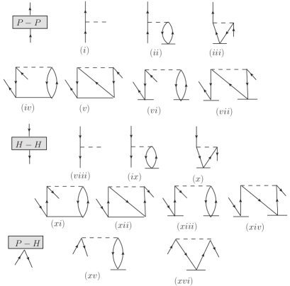
Figure 2: Effective one-body intermediate diagrams constructed from $\overline{H_{N}^{DC}}$ in order to evaluate the $T^{(1)}$ amplitudes. Here broken lines represent the Coulomb interaction and the solid line without arrows symbolize the $T^{(0)}$ operators.

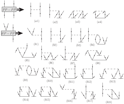
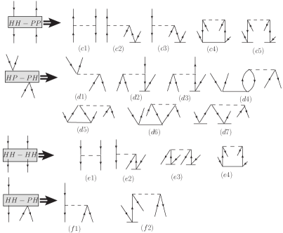
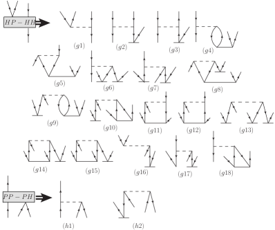
Figure 3: Effective two-body intermediate diagrams constructed from $\overline{H_{N}^{DC}}$ in order to evaluate the $T^{(1)}$ amplitudes. Here broken lines represent the Coulomb interaction and the solid line without arrows symbolize the $T^{(0)}$ operators.

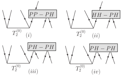
Figure 4: Effective three-body intermediate diagrams constructed from $\overline{H_{N}^{DC}}T_{2}^{(0)}$ to solve for the $T^{(1)}$ amplitudes.

In the CC method, we express the unperturbed atomic wave function as

$$|\Psi_{0}^{(0)}\rangle = \Omega_{\text{RCC}}^{(0)}|\Phi_{0}\rangle$$ (29)

$$= \sum_{k}^{\infty}\Omega_{\text{RCC}}^{(k,0)}|\Phi_{0}\rangle$$

$$= e^{T^{(0)}}|\Phi_{0}\rangle$$

and the first order perturbed wave function as yashpal-polz

$$|\Psi_{0}^{(1)}\rangle = \Omega_{\text{RCC}}^{(1)}|\Phi_{0}\rangle$$ (30)

$$= \sum_{k}^{\infty}\Omega_{\text{RCC}}^{(k,1)}|\Phi_{0}\rangle$$

$$= e^{T^{(0)}}T^{(1)}|\Phi_{0}\rangle,$$

where $T^{(0)}$ and $T^{(1)}$ are the excitation operators from the reference state $|\Phi_{0}\rangle$ that take care of contributions from the Coulomb interactions and Coulomb interactions along with from the perturbed $D$ operator, respectively.

The amplitudes of the excitation $T^{(0)}$ and $T^{(1)}$ operators are determined using the equations

$$\langle\Phi_{0}^{\tau}|\overline{H_{N}^{DC}}|\Phi_{0}\rangle = 0$$ (31)

and

$$\langle\Phi_{0}^{\tau}|\overline{H_{N}^{DC}}T^{(1)}|\Phi_{0}\rangle = -\langle\Phi_{0}^{\tau}|\overline{D}|\Phi_{0}\rangle,$$ (32)

where $H_{N}^{DC}$ is the normal ordered DC Hamiltonian, $\overline{O}=(Oe^{T^{(0)}})_{con}$ with $con$ means only the connected terms and $|\Phi_{0}^{\tau}\rangle$ corresponds to the excited configurations with $\tau$ referring to level of excitations from $|\Phi_{0}\rangle$. In our calculations, we only consider the singly and doubly excited configurations ($\tau=1,2$) by defining

$$T^{(0)} = T_{1}^{(0)}+T_{2}^{(0)}\ \ \ \ \text{and}\ \ \ \ T^{(1)}=T_{1}^{(1)}+T_{2}^{(1)},$$ (33)

which is known as the CCSD method in the literature. When we consider the approximation $\overline{O}=O+OT$, we refer it as the LCCSD method.

To carry out calculations in an optimum computational requirements, we construct the intermediate diagrams for the effective operators by dividing the non-linear CC terms. The intermediate diagrams for the computation of the $T^{(0)}$ amplitudes are described at length in our previous work yashpal-polz . Here, we discuss only about the intermediate diagrams used for the evaluation of the $T^{(1)}$ amplitudes. For this purpose, we express $\overline{H_{N}^{DC}}$ into the effective one-body, two-body and three-body diagrams. It is worth while to note that there is a technical difference between the construction of the intermediate diagrams from $\overline{H_{N}^{DC}}$ for the $T^{(0)}$ and $T^{(1)}$ amplitude solving equations. In Eq. (32), $\overline{H_{N}^{DC}}$ contains all the non-linear terms while for solving Eq. (31) it is required to express as $\overline{H_{N}^{DC}}=\overline{H_{N}^{DC}}^{\prime}\otimes T_{\tau}$. Thus the intermediate diagrams in this case are comprised terms from $\overline{H_{N}^{DC}}^{\prime}$ which requires special scrutiny of the diagrams to avoid repetition in the singles and doubles amplitude calculations. The effective intermediate diagrams used for the $T^{(1)}$ amplitude determining equations are shown in Figs. 2, 3 and 4. These effective diagrams are finally connected with the respective $T^{(1)}$ operators to obtain the amplitudes of the singles and doubles excitations and the corresponding diagrams are presented in Figs. 6 and 7. Contributions from the terms of $\overline{D}$ are evaluated directly for the $T^{(1)}$ amplitude calculations and the corresponding diagrams are shown in Figs. 8 and 9.

In order to estimate the dominant contributions from the triple excited configurations, we define an excitation operator perturbatively in the CC framework as following

$$T_{3}^{(0),pert}=\frac{1}{3!}\sum_{abc}^{pqr}\frac{(\overline{H_{N}^{DC}}T_{2}^{(0)})_{abc}^{pqr}}{\epsilon_{a}+\epsilon_{b}+\epsilon_{c}-\epsilon_{p}-\epsilon_{q}-\epsilon_{r}}$$ (34)

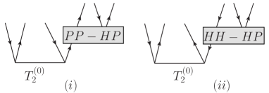
Figure 5: Diagrams representing $T_{3}^{(0),pert}$ operator.

which diagrammatically shown in Fig. 5 and contract it with the $D$ operator to calculate the amplitudes of the $T_{2}^{(1)}$ perturbed CC operator in a self-consistent procedure considering it in Eq. (32) as part of $\overline{D}$. We refer this approach as the CCSD_pT method in this work.

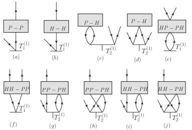
Figure 6: Final contributing diagrams for the $T_{1}^{(1)}$ amplitude calculations which are constructed by the contraction of effective one and two body intermediate diagrams with $T^{(1)}1$ operators.

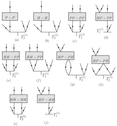
Figure 7: Final contributing diagrams for the $T_{2}^{(1)}$ amplitude calculations which are constructed by the contraction of effective one and two body intermediate diagrams with $T^{(1)}1$ operators.

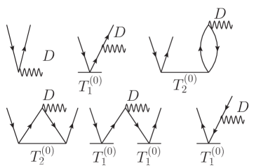
Figure 8: Single excitation diagrams from $\overline{D}$ that contribute to the calculations of the $T^{(1)}$ amplitudes.

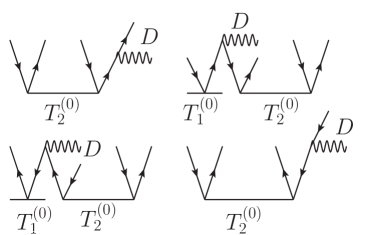
Figure 9: Double excitation diagrams from $\overline{D}$ that contribute to the calculations of the $T^{(1)}$ amplitudes.

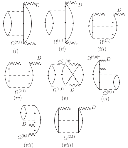
Figure 10: Few significantly contributing non-RPA type MBPT(3) diagrams.

Using the above formulation, the expression for the polarizability is given by yashpal-polz

$$\alpha = 2\frac{\langle\Phi_{0}|\Omega_{\text{RCC}}^{(0)\dagger}D\Omega_{\text{RCC}}^{(1)}|\Phi_{0}\rangle}{\langle\Phi_{0}|\Omega_{\text{RCC}}^{(0)\dagger}\Omega_{\text{RCC}}^{(0)}|\Phi_{0}\rangle}$$ (35)

$$= 2\frac{\langle\Phi_{0}|e^{T^{(0)\dagger}}De^{T^{(0)}}T^{(1)}|\Phi_{0}\rangle}{\langle\Phi_{0}|e^{T^{(0)\dagger}}e^{T^{(0)}}|\Phi_{0}\rangle}$$

$$= 2\langle\Phi_{0}|(\overbrace{D^{(0)}}T^{(1)})_{con}|\Phi_{0}\rangle,$$

where $\overbrace{D^{(0)}}=e^{T^{\dagger{(0)}}}De^{T^{(0)}}$ is a non-truncating series. In the LCCSD method, we only consider the terms $\overbrace{D^{(0)}}=O+OT^{(0)}+T^{\dagger{(0)}}O+T^{\dagger{(0)}}OT^{(0)}$. Computational steps to account all the significant contributions from $\overbrace{D_{N}^{(0)}}$ have been described in detail in our previous work yashpal-polz .

IV Results and Discussion

Table 1: Results for the dipole polarizabilities from our CCSD_pT method along with the available measurements and others calculations. Uncertainties in the results are given in the parentheses and the references are cited in the square brackets.

System	Present	Others
	CCSDpT	Theory	Experiment
B+	10.395(20)	9.448epstein , 9.64(3)cheng1
		9.624safronova
C2+	4.244(10)	3.347epstein
Al+	24.26(4)	24.2archibong , 24.14(12)mitroy	a24.20(75)reshetnikov
		24.12hamonou , 24.048 safronova
		24.14(8) kallay
		24.065(410)yu
Si2+	11.88(25)	11.688mitroy1	11.666(4)komara
		11.75hamonou	b11.669(9)mitroy1
Zn	38.666(35)	38.12ye , 39.2(8)goebel	38.8(8)goebel
		38.4roos , 37.9kello ,
		38.01seth
Ga+	18.441(20)	17.95(34)cheng
Ge2+	10.883(10)
Cd	45.856(42)	46.25seth , 44.63ye	49.65(1.49)goebel1
		46.8kello , 46.9roos
In+	24.11(15)	24.01 safronova
Sn2+	15.526(22)

a Estimated from the measured oscillator strengths.

b Obtained by reanalyzing data of Ref. komara .

Our final results using the CCSD_pT method along with the available experimental values for Al⁺, Si²⁺, Zn and Cd and from the other calculations are given in Table 1. To ascertain lucidity in the accuracies of the results from our calculations, we also provide the estimated uncertainties associated with our results by estimating contributions from various neglected sources and give them in the parentheses alongside the CCSD_pT results in above table. The value that is referred to as the experimental results for Al⁺ is not directly obtained from the measurement, rather it is estimated by summing over the experimental values of the oscillator strengths and has relatively large uncertainty compared to some of the reported calculations reshetnikov . There are two high-precision results reported as the experimental values for the Si²⁺ ion komara ; mitroy1 , however the value reported in komara is obtained from the direct analysis of the energy intervals measurement using the resonant Stark ionization spectroscopy (RESIS) technique while the other value mitroy1 is reported by reanalyzing the data of Ref. komara ; which is about 0.03% larger than the former value. The only available experimental result of the ground state $\alpha$ of Zn is measured using an interferometric technique by Goebel et al. goebel . Similarly there is also one measurement of $\alpha$ available for Cd using a technique of dispersive Fourier-transform spectroscopy, but the reported uncertainty in this experimental value is comparatively large goebel1 . Nevertheless when we compare our CCSD_pT results with all these experimental values, they match very well within their reported error bars except for Cd. In fact, our calculations are more precise in all the systems apart for the Si²⁺ ion. There are no experimental results available for the other considered ions to compare them against our calculations.

There are also a number of calculations of $\alpha$ available by many groups using varieties of many-body approaches among which some of them are based on either the lower order methods or considering the non-relativistic mechanics. An old calculation of $\alpha$ in B⁺ was reported by Epstein et al epstein based on the coupled perturbed Hartree-Fock (CHF) method while Cheng et al had employed a configuration interaction method considering a semi-empirical core-polarization potential (CICP method) to evaluate it more precisely cheng1 . Later Safronova et al used a combined CI and LCCSD methods (CI$+$all order method) to determine $\alpha$ of B⁺ ion safronova . However, the CCSD_pT result seems to be larger than all other calculations. Our analysis suggests that the differences in these results are mainly due to inclusion of the pair-correlation effects to all orders in our CC method. In C²⁺ ion, we find only one theoretical result reported by Epstein et al using the same CHF method. Our result for C⁺² is also slightly larger than the value reported by the above calculation. Till date Al⁺ is the most precise ion clock in the world rosenband2 for which a couple of high-precision calculations have been reported on the determination of $\alpha$ of this ion by attempting to push down the uncertainty in the black-body radiation (BBR) shift of the respective ion-clock transition kallay ; safronova ; yu . Among them calculations carried out by Mihaly et al is based on the relativistic CC method considering up to quadrupole excitations and finite field approach kallay . However, calculations carried out in this work is based on the Cartesian coordinate system and minimizing the energies in the numerical differentiation approach in contrast to the present CCSD_pT method, where the matrix elements of $D$ are evaluated in the spherical coordinate system. Calculations reported by Yu et al is using the same approach of Ref. kallay , but by considering a different set of single particle orbitals yu . Safronova et al have employed the CI$+$all order approach to calculate $\alpha$ of Al⁺. There are also other theoretical results have been reported based on varieties of many-body methods such as CCSD, CICP, CI etc. both in the non-relativistic and relativistic mechanics archibong ; mitroy ; hamonou . We find an excellent agreement among all the theoretical results. Some of these methods have also been employed to calculate $\alpha$ of Si²⁺ mitroy ; hamonou which are in perfect agreement with the experimental results. However, our CCSD_pT value seems to be little larger then the experimental result but falls within the estimated uncertainty. We found only one more calculation of $\alpha$ in Ga⁺ using the CICP method cheng to compare with our result. Although values from both the calculations are very close but they do not agree within their reported uncertainties. Calculations in Cd are reported by many groups including the latest one using the Douglas-Kroll-Hess (DKH) Hamiltonian by Roos et al roos . Calculations carried out by Ye et al ye is based on the relativistic formalism in the CICP method. All the theoretical results are consistent and show good agreement with each other suggesting that the experimental result could have been overestimated. Therefore it is important to have another measurement of the polarizability of Cd to resolve this ambiguity. Again there has also been an effort made for the precise determination of $\alpha$ in In⁺ to estimate the BBR shift accurately for its proposed atomic clock transition safronova . Our result agrees nicely with this calculation. As discussed earlier, calculations carried out in safronova are based on the CI$+$all order method. We could not find any other calculations of $\alpha$ of the ground states of the Ge²⁺ and Sn²⁺ ions to make comparative analyses with our results.

Table 2: Dipole polarizabilities of the considered atomic systems are presented using different many-body methods.

System	DF	MBPT(3)	RPA	LCCSD	CCSD
B+	8.142	9.720	11.374	11.875	10.413
C2+	3.282	3.804	4.503	4.886	4.213
Al+	19.514	21.752	26.289	26.118	24.299
Si2+	9.683	10.482	12.476	12.847	11.893
Zn	37.317	34.421	50.846	38.739	38.701
Ga+	17.148	15.796	21.780	19.138	18.455
Ge2+	10.085	8.884	12.011	11.520	10.890
Cd	49.647	35.728	63.743	45.086	45.898
In+	25.734	18.374	29.570	25.360	24.246
Sn2+	16.445	12.095	17.941	15.978	15.537

To assimilate the underlying roles of the electron correlation behavior in the evaluation of $\alpha$ of the ground states of the considered systems, we systematically present the calculated values of the dipole polarizabilities in Table 2 from the DF, MBPT(3), RPA, LCCSD and CCSD methods. So, the differences between the CCSD results and the values quoted from the CCSD_pT method in Table 1 are the contributions from the partial triple excitations. Obviously, these differences are small in magnitude implying that the contributions from the unaccounted higher order excitations are very small. The lowest order DF results are smaller in magnitudes in the lighter systems but their trends revert in the Cd isoelectronic systems with respect to their corresponding CCSD results. Also, the MBPT(3) results do not follow a steady trend. In the B⁺, C²⁺, Al⁺ and Si²⁺ ions, the correlation effects enhance the $\alpha$ values in the MBPT(3) method from their DF results while the MBPT(3) results are smaller than the DF values in the other systems. As has been stated earlier RPA is a non-perturbative method embracing the core-polarization effects to all orders, but we find that the results are over estimated in this method compared to the CCSD results; more precisely from the experimental values given in Table 1. We understand these differences as the contributions from the pair-correlation effects that are absent in the RPA method, but they are accounted intrinsically to all orders as the integral part of the CCSD method. The role of the pair-correlation effects in the determination of $\alpha$ are verified by examining contributions from the individual MBPT(3) diagrams. The dominant contributing non-RPA diagrams appearing in the MBPT(3) method that take care of the pair-correlation effects are shown in Fig. 10. In fact, contributions from these non-RPA diagrams are found to be larger than the differences between the RPA and CCSD results reported in Table 2. This finding advocates that there are large cancellations among the lower order and higher order pair-correlation contributions in the CCSD method bestowing modest size of contributions to $\alpha$, but they appear to be very significant in the heavier systems to attribute accuracies in the results. To demonstrate the roles of the non-linear terms to procure high precision $\alpha$ values in the considered ions, we have also given the results from the LCCSD method in the above table. Although LCCSD is an all order perturbative method, but it clearly omits higher order core-polarization and pair-correlation effects that crop-up through the non-linear terms involving $T^{(0)}T^{(0)}$ or higher powers of $T^{(0)}$. Consequently, this method also over estimates the results like the RPA method. The LCCSD results in B⁺ and C²⁺ are larger than the RPA values, but the LCCSD values are smaller than the RPA results in the other cases. This clearly demonstrates intermittent trends of the correlation effects in the determination of $\alpha$ of the systems belonging to a particular group of elements in the periodic table to another through a given many-body method as well as when they are studied using the methods with different levels of approximations. To manifest contributions from the correlations effects through various many-body methods quantitatively, we portray the results obtained for $\alpha$ of the considered systems using these methods in a histogram as shown in Fig. 11. This clearly bespeaks about the lopsided trend in the estimation of $\alpha$ of the considered systems. Again, we also plot the $\alpha$ values of the singly and doubly charged ions separately in Figs. 12 and 13 in order to make a comparative analysis in the propagation of correlation effects through the employed methods in these elements that belong to two different groups of the periodic table. This figure shows that the contributions from the correlation effects in the singly charged and doubly charged ions do not exactly follow similar trends.

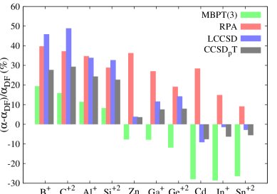
Figure 11: (color online) Histogram showing $(\alpha-\alpha_{D})/\alpha_{D}$ (in %) with different many-body methods against the considered atomic systems.

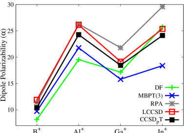
Figure 12: (color online) Trends in the calculations of dipole polarizabilities ($\alpha$) from the employed many-body methods in the considered singly charged ions.

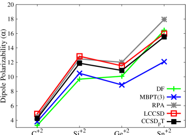
Figure 13: (color online) Trends in the calculations of dipole polarizabilities ($\alpha$) from the employed many-body methods in the considered doubly charged ions.

Finally, we would like to discuss about the trends in the correlation effects coming through various CCSD_pT terms. We give contributions explicitly from the individual CC terms of linear form and the rest as “Others” in Table 3. Clearly, this table shows that the first term $DT^{(1)}$ gives the dominant contributions as it subsumes all the leading order core-polarization and pair-correlation effects along with the DF result. The next dominant contributing term is $T_{2}^{(0)\dagger}DT_{1}^{(1)}$ which incorporates some contributions from the correlation effects emanated at the MBPT(2) level and possess opposite signs from the $DT^{(1)}$ contributions causing cancellations among them. It is also worthy to mention that contributions coming from the $T_{2}^{(0)\dagger}DT_{2}^{(1)}$ term corresponds to the higher order perturbation and also accounts contributions from the doubly excited intermediate states. As seen from the table, these contributions are non-negligible suggesting that they should also be estimated accurately for accomplishing high precision results and the sum-over-states approach may not be able to augment these contributions suitably in the considered systems. Contributions from the other non-linear CC terms at the final property evaluation level seem to be slender, although the differences between the LCCSD and CCSD results emphasis their importance for accurate calculations of the atomic wave functions in the considered systems.

Table 3: Contributions to the $\alpha$ of the ground state of considered atomic systems from various CCSD_pT terms.

System	$DT_{1}^{(1)}$	$T_{1}^{(0)\dagger}DT_{1}^{(1)}$	$T_{2}^{(0)\dagger}DT_{1}^{(1)}$	$T_{2}^{(0)\dagger}DT_{2}^{(1)}$	Others
	+c.c	+c.c	+c.c	+c.c
B+	10.848	$-$0.194	$-$1.679	0.774	0.646
C2+	4.392	$-$0.047	$-$0.668	0.274	0.29
Al+	25.855	$-$0.519	$-$3.166	1.523	0.567
Si2+	12.589	$-$0.160	$-$1.475	0.666	0.260
Zn	43.812	$-$2.458	$-$5.286	2.047	0.551
Ga+	20.223	$-$0.545	$-$2.409	0.837	0.335
Ge2+	11.846	$-$0.198	$-$1.363	0.476	0.122
Cd	52.963	$-$3.346	$-$6.985	2.262	0.962
In+	27.134	$-$0.882	$-$3.647	1.064	0.441
Sn2+	17.249	$-$0.366	$-$2.286	0.603	0.326

V Conclusion

We have employed a variety of many body methods to incorporate the correlation effects at different levels of approximations to unravel the role of the correlation effects and follow-up their trends to achieve very accurate calculations of the dipole polarizabilities of three groups of elements in the periodic table. We find the patterns in which the correlation effects behave with respect to the mean-field level of calculations are divergent in the individual isoelectronic systems through a particular employed many-body method. Also, our calculations reveal that inclusion of both the core-polarization and pair-correlation effects to all orders are equally important for securing high precision dipole polarizabilities in the considered systems and the core-polarization effects play the pivotal role among them. Contributions from the doubly excited states are found to be non-negligible implying that a sum-over-states approach may not be pertinent to carry out these studies. Our results obtained using the singles, doubles and important triples approximation in the coupled-cluster method agree very well with the available experimental values in some of the systems except for cadmium. In fact none of the reported theoretical results for cadmium agree with the measurement, however there seem to be reasonable agreement among all theoretical results. This urges for further experimental investigation of the cadmium result. In few systems, there are no experimental results available yet and the reported precise values in the present work can be served as exemplars for their prospective measurements.

VI Acknowledgment

BKS was supported partly by INSA-JSPS under project no. IA/INSA-JSPS Project/2013-2016/February 28, 2013/4098. The computations reported in the present work were carried out using the 3TFLOP HPC cluster at Physical Research Laboratory, Ahmedabad.

References

- (1) S. A. Diddams et. al., Science 293, 825 (2001).
- (2) P. Gill et. al., Meas. Sci. Technol. 14, 1174 (2003).
- (3) P. Gill, Metrologia 42, S125 (2005).
- (4) T. Rosenband et. al., Phys. Rev Lett. 98, 220801 (2007).
- (5) T. Rosenband et. al., Science 319, 1808 (2008).
- (6) K. D. Bonin and V. V. Kresin, Electric dipole polarizabilities of atoms, molecules and clusters, World Scientific, Singapore (1997).
- (7) C. J. Pethick and H. Smith, Bose-Einstein Condensation in Dilute Gases, Cambridge University Press, Cambridge, UK (2008).
- (8) A. A. Madej and J. E. Bernard, Frequency Measurement and Control, edited by Andre N. Luiten, Topics in Applied Physics, v. 79, (Springer, Berlin, 2001), pp. 153–195.
- (9) W. D. Hall and J. C. Zorn, Phys. Rev. A 10, 1141 (1974).
- (10) R. W. Molof, H. L. Schwartz, T. M. Miller, and B. Bederson, Phys. Rev. A 10, 1131 (1974).
- (11) T. M. Miller and B. Bederson, Phys. Rev. A 14, 1572 (1976).
- (12) H. L. Schwartz, T. M. Miller, and B. Bederson, Phys. Rev. A 10, 1924 (1974).
- (13) A. D. Cronin, J. Schmiedmayer, and D. E. Pritchard, Rev. Mod. Phys. 81, 1051 (2009).
- (14) C. R. Ekstrom, J. Schmiedmayer, M. S. Chapman, T. D. Hammond, and D. E. Pritchard, Phys. Rev. A 51, 3883 (1995).
- (15) J. M. Amini and H. Gould, Phys. Rev. Lett. 91, 153001 (Oct 2003).
- (16) A. Dalgarno, Adv. Phys. 11, 281 (1962).
- (17) A. Dalgarno and H. A. J. McIntyre, Proc. Roy. Soc. 85, 47 (1965).
- (18) H. J. Monkhorst, Int. J. Quantum Chem. 12(S11), 421 (1977).
- (19) E. Dalgaard and H. J. Monkhorst, Phys. Rev. A 28, 1217 (1983).
- (20) B. Kundu and D Mukherjee, Chem. Phys. Lett. 179, 468 (1991).
- (21) H. Koch, R. Kobayashi, A. Sanchez de Merśs, and P. Jørgensen, J. Chem. Phys. 100, 4393 (1994).
- (22) R. Kobayashi, H. Koch, and P. Jørgensen, J. Chem. Phys 101, 4956 (1994).
- (23) B. Datta , P. Sen, and D. Mukherjee, J. Phys. Chem. 99, 6441 (1995).
- (24) K. Kowalski, J. R. Hammond, and W. A. de Jong, J. Chem. Phys. 127, 164105 (2007).
- (25) J. R. Hammond, Coupled-cluster Response Theory: Parallel Algorithms and Novel Applications, PhD thesis submitted to Department of Chemistry, The University of Chicago, USA (2009).
- (26) I. S. Lim and P. Schwerdtfeger, Phys. Rev. A 70, 062501 (2004).
- (27) I. S. Lim, H. Stoll, and P. Schwerdtfeger, J. Chem. Phys. 124, 034107 (2006).
- (28) B. K. Sahoo, Chem. Phys. Lett. 448, 144 (2007).
- (29) B. K. Sahoo and B. P. Das, Phys. Rev. A 77, 062516 (2008).
- (30) Y. Singh, B. K. Sahoo, and B. P. Das, Phys. Rev. A 88, 062504 (2013).
- (31) S. Chattopadhyay, B. K. Mani, and D. Angom, Phys. Rev. A 87, 062504 (2013 ).
- (32) S. Chattopadhyay, B. K. Mani, and D. Angom, Phys. Rev. A 89, 022506 (2014).
- (33) I. Lindgren and J. Morrison, Atomic Many-Body Theory, Second Edition, Springer-Verlag, Berlin, Germany (1986).
- (34) S. T. Epstein and R. E. Johnson, J. Chem. Phys. 47, 2275 (1967).
- (35) Y. Cheng and J. Mitroy, Phys. Rev. A 86, 052505 (2012).
- (36) M. S. Safronova, M. G. Kozlov, and C. W. Clark, Phys. Rev. Lett. 107, 143006 (2011).
- (37) E. F. Archibong, and A. J. Thakkar, Phys. Rev. A 44, 5478 (1991).
- (38) J. Mitroy, J. Y. Zhang, M. W. J. Bromley, and K. G. Rollin, Eur. Phys. J. D 53, 15 (2009).
- (39) N. Reshetnikov, L. J. Curtis, M. S. Brown, and R. E. Irving, Phys. Scr. 77, 015301 (2008).
- (40) L. Hamonou and A. Hibbert, J. Phys. B 41, 245004 (2008).
- (41) M. Kállay, H. S. Nataraj, B. K. Sahoo, B. P. Das, and L. Visscher, Phys. Rev. A 83, 030503(R) (2011).
- (42) Y. Yu, B. Suo, and H. Fan, Phys. Rev. A 88, 052518 (2013).
- (43) J. Mitroy, Phys. Rev. A 78, 052515 (2008).
- (44) R. A. Komara, M. A. Gearba, C. W. Fehrenbach and S. R. Lundeen, J. Phys. B 38, S87 (2005).
- (45) A. Ye and G. Wang, Phys. Rev. A 78, 014502 (2008).
- (46) D. Goebel, U. Hohm, and G. Maroulis, Phys. Rev. A 54, 1973 (1996).
- (47) B. O. Roos, R. Lindh, P-ÅA. Malmqvist, V. Veryazov, and P. -O. Widmark, J. Phys. Chem. A 109, 6575 (2005).
- (48) V. Kellö and A. J. Sadlej, Theor. Chim. Acta 91, 353 (1995).
- (49) M. Seth, P. Schwerdtfeger, and M. Dolg, J. Chem. Phys. 106, 3623 (1997).
- (50) Y. Cheng and J. Mitroy, J. Phys. B 46, 185004 (2013).
- (51) D. Goebel and U. Hohm Phys. Rev. A 52, 3691 (1995).