Orbital-free density functional theory of out-of-plane charge screening in graphene

Abstract

We propose a density functional theory of Thomas-Fermi-Dirac-von Weizsäcker type to describe the response of a single layer of graphene resting on a dielectric substrate to a point charge or a collection of charges some distance away from the layer. We formulate a variational setting in which the proposed energy functional admits minimizers, both in the case of free graphene layers and under back-gating. We further provide conditions under which those minimizers are unique and correspond to configurations consisting of inhomogeneous density profiles of charge carrier of only one type. The associated Euler-Lagrange equation for the charge density is also obtained, and uniqueness, regularity and decay of the minimizers are proved under general conditions. In addition, a bifurcation from zero to non-zero response at a finite threshold value of the external charge is proved.

1 Introduction

Graphene is a two-dimensional monolayer of carbon atoms arranged into a perfect honeycomb lattice novoselov04. It has received a huge amount of attention in recent years, both as a very promising material for nanotechnology applications and as a model system with pronounced quantum mechanical properties (for reviews, see geim07; castroneto09; abergel10). The current interest in graphene stems from its very unusual electronic properties closely related to the symmetry and the two-dimensional character of the underlying crystalline lattice, into which the carbon atoms arrange themselves. A free-standing graphene layer acts as a semi-metal, in which the low energy charge carrying quasiparticles (electrons and holes) behave to a first approximation as massless fermions obeying a two-dimensional relativistic Dirac equation wallace47; fefferman12; fefferman12a. Hence, their kinetic energy is proportional to their quasi-momentum:

$$\varepsilon_{\mathbf{k}}=\pm\hbar v_{F}|\mathbf{k}|,$$ (1.1)

where $v_{F}\simeq 1\times 10^{8}$ cm/s is the Fermi velocity, $\mathbf{k}$ is the wave vector and “$\pm$” stands for electrons and holes, respectively. This equation is valid for $|\mathbf{k}|\ll a_{0}^{-1}$, where $a_{0}\simeq 1.42\,\mathring{A}$ is the nearest-neighbor distance between the carbon atoms in the graphene lattice (without taking into account the effect of the velocity renormalization gonzalez94; KotovUchoa:12; martin08; reed10; sodemann12; yu13).

In contrast to the fermions with non-zero effective mass in the usual metals or semiconductors, in graphene the effect of interparticle Coulomb repulsion does not decrease with increasing carrier density KotovUchoa:12. This can already be seen from simple dimensional considerations: according to (1.1) a single particle whose wave function is localized into a wave packet of radius $\sim r$ would have kinetic energy $E_{kin}\sim\hbar v_{F}/r$, while the energy of Coulomb repulsion per particle (in CGS units) is $E_{Coulomb}\sim e^{2}/(\epsilon_{d}r)$, where $e>0$ is the elementary charge and $\epsilon_{d}$ is the effective dielectric constant in the presence of a substrate. Thus their ratio $\alpha=e^{2}/(\epsilon_{d}\hbar v_{F})$, which characterizes the relative strength of the Coulombic interaction, is a constant independent of $r$, and, furthermore, we have $\alpha\simeq 2.2$ for $\epsilon_{d}=1$, indicating the non-perturbative role of the Coulombic interaction in the absence of a strong dielectric background.

The scaling argument above can also be applied to an electron obeying (1.1) in an attractive potential of a positively charged ion. When the valence $Z$ of the ion increases, the potential energy $E_{pot}\sim-Ze^{2}/r$ of the attractive interaction between the electron and the ion always overcomes the kinetic energy. At the single particle level this effect results in non-existence of single particle ground states for the relativistic Dirac-Kepler problem shytov07, which is somewhat similar to the phenomenon of relativistic atomic collapse lieb88. In a more realistic multiparticle setting the situation is more complicated due to strongly correlated many-body effects involving both the electrons and holes. In fact, exactly how the carriers in graphene screen a charged impurity is a subject of an ongoing debate, with qualitatively different predictions for the behavior of the screening charge density and the total electrostatic potential coming from different theories.

Early studies of screening of the electric field from point charges in graphene go back to the work of DiVincenzo and Mele, who used a self-consistent Hartree-type model to analyze the electron response to interlayer charges in intercalated graphite compounds divincenzo84. They found a surprising result that the screening electron density decays as $1/r^{2}$ (to within an undetermined logarithmic factor), indicating that the screening charge is considerably spread out laterally within the graphene layer. They also made a similar conclusion from the analysis of the Thomas-Fermi equations for massless relativistic fermions and contrasted it with the $1/r^{3}$ behavior expected from the image charge on an equipotential plane in the case of perfect screening. In sharp contrast, Shung performed an analysis of the dielectric susceptibility of intercalated graphite compounds using linear response theory shung86. His calculation implies that in the absence of doping only partial screening of an impurity should occur and that the electron system should behave effectively as a dielectric medium due to the excitation of virtual electron-hole pairs, which has an effect of renormalizing the value of $\epsilon_{d}$ (see also gonzalez94; Ando:06; HwangDasSarma:07; KotovUchoa:12 for further discussions). He also commented that the nonlinear effects are of major importance in the screening, which explains the different results he had for linear response comparing with the Thomas-Fermi result in divincenzo84.

More recently, Katsnelson computed the asymptotic behavior of the screening charge density for a charged impurity within the Thomas-Fermi theory of massless relativistic fermions with a lattice cutoff at short scales Katsnelson:06. He found that the screening charge density should behave as $1/(r\ln r)^{2}$ far from the impurity, refining earlier results of divincenzo84 and demonstrating the importance of nonlinear screening effects in graphene. Fogler, Novikov and Shklovskii further considered the effect of an out-of-plane hypercritical charge $Z\gg 1$ on the electron system in a graphene layer and argued for perfect screening ($1/r^{3}$ behavior of the screening charge density and constant electrostatic potential in the layer) fogler07. They also argued for a crossover between perfect screening in the near field tail, Thomas-Fermi screening ($1/(r\ln r)^{2}$ behavior of the screening charge density and $1/(r\ln r)$ decay of the electrostatic potential in the layer) in the far field tail, and partial screening (dielectric response with no screening charge and $1/r$ decay of the electrostatic potential) in the very far tail for certain ranges of $Z$ and $\alpha$. We also note that a recent result indicates that in the Hartree-Fock approximation the relative dielectric constant of graphene is, somewhat surprisingly, equal to unity in the Hartree-Fock theory, implying that the total induced charge from a charged impurity in graphene is zero (no partial screening or effectively very weak screening due to the slow decay) HainzlLewinSparber:2012.

The differing conclusions of the above works indicate a very delicate nature of the problem of screening in graphene (see also the discussion in KotovUchoa:12 and further references therein). One reason is the precise tuning of the kinetic energy, the Coulombic attraction of electrons to the impurity and the Coulombic repulsion between electrons, which is already evident from the scaling argument presented earlier. Another reason is that the studies mentioned above do not account for the correlation effects. While it is believed that exchange does not play a significant effect in graphene, correlations between electrons and holes due to their Coulombic attraction (excitonic effects) may have an effect on the nature of the response beyond random phase approximation KotovUchoa:12; abergel09; abergel10; martin08; reed10; sodemann12; wang12; yu13. Finally, the third reason is that in view of the crucial role played by nonlinear and nonlocal effects for charge carrier behavior in graphene the analysis of the problem, both mathematical and numerical, becomes rather non-trivial.

Our approach to the problem of screening of point charges by a graphene layer is via introducing a Thomas-Fermi-Dirac-von Weizsäcker (TFDW) type energy for massless relativistic fermions and studying the associated variational problem. The considered energy functional is a variant of an orbital-free density functional theory (for a recent Kohn-Sham-type density functional theory see polini08) that models the exchange and correlation effects by renormalizing the corresponding coefficients of the Thomas-Fermi theory for the system of non-interacting massless relativistic fermions and introducing a non-local analog of the von Weizsäcker term in the usual TFDW model of a non-relativistic electron gas Lieb:81; lebris05. For simplicity, we begin by treating the problem of the influence of a single point charge $+Ze$ located at distance $d\gg a_{0}$ away from the graphene layer on the electrons in the layer. It may either correspond to the effect of a charge placed on a gate separated from the graphene layer by a layer of insulator in the context of graphene-based nanodevices, or it may correspond to an imbedded charged impurity or a cluster of impurities within the dielectric substrate. After a suitable rescaling, the TFDW energy for graphene at the neutrality point in the presence of an impurity takes the following form:

$$E_{0}(\rho)=a\int_{\mathbb{R}^{2}}\left|\nabla^{\frac{1}{2}}\bigl{(}\sqrt{\left\lvert\rho(x)\right\rvert}\operatorname{sgn}(\rho(x))\bigr{)}\right|^{2}\,\mathrm{d}^{2}x+\frac{2}{3}\int_{\mathbb{R}^{2}}\left\lvert\rho(x)\right\rvert^{3/2}\,\mathrm{d}^{2}x\\ -\int_{\mathbb{R}^{2}}\frac{\rho(x)}{\bigl{(}1+\left\lvert x\right\rvert^{2}\bigr{)}^{1/2}}\,\mathrm{d}^{2}x+\frac{b}{2}\iint_{\mathbb{R}^{2}\times\mathbb{R}^{2}}\frac{\rho(x)\rho(y)}{\left\lvert x-y\right\rvert}\,\mathrm{d}^{2}x\,\mathrm{d}^{2}y.$$ (1.2)

Here $\rho(x)$ is the signed particle density, with $\rho>0$ corresponding to electrons and $\rho<0$ corresponding to holes, and $a\geq 0$ and $b\geq 0$ are two dimensionless parameters characterizing the model. Note that in the case of $a=0$ we recover the usual Thomas-Fermi model for graphene. The case of $b=0$ would correspond to a model system of non-interacting massless relativistic fermions in an external potential. The meaning of each term in (1.2) and the relation to the original physical parameters is explained in Sec. 2. Let us point out the unusual non-local nature of both the first and the last terms in (1.2). The first term involves the homogeneous $H^{1/2}(\mathbb{R}^{2})$ norm squared $\int_{\mathbb{R}^{2}}|\nabla^{\frac{1}{2}}u|^{2}\,\,\mathrm{d}^{2}x$ of $u=\rho/|\rho|^{1/2}$, while the last term involves the homogeneous $H^{-1/2}(\mathbb{R}^{2})$ norm squared of $\rho$. This is in contrast to the conventional TFDW models of massive non-relativistic fermions, in which the first term involves the homogeneous $H^{1}$ norm and the last term involves the homogeneous $H^{-1}$ norm, respectively. The difference in the first term has to do with the relativistic character of the dispersion relation for quasiparticles in graphene at low energies given by (1.1), while the difference in the last term reflects the three-dimensional character of Coulomb interaction and the two-dimensional character of the charge density. We point out that a von Weizsäcker-type term similar to the first term in (1.2) appeared in the studies of stability of relativistic matter (see, e.g., lieb96 and references therein). We also note that our model is different from the ultrarelativistic Thomas-Fermi-von Weizsäcker model studied in EngelDreizler:87; EngelDreizler:88; BenguriaLossSiedentop:2008, where a local gradient term in the kinetic energy for massless relativistic fermions in three space dimensions was used. An analogous term for graphene would have been $\int_{\mathbb{R}^{2}}\bigl{|}\nabla\left\lvert\rho\right\rvert^{1/4}\bigr{|}^{2}\,\mathrm{d}^{2}x$ (see Sec. 2 for the explanation of our choice of the non-local term).

The model above is easily generalized to include a collection of point charges or a localized distribution of charges some distance away from the graphene layer. If

$$V(x)=-\int_{\mathbb{R}^{3}}{\,\mathrm{d}\mu(y,z)\over(|1+z|^{2}+|x-y|^{2})^{1/2}},$$ (1.3)

where $\mu(y,z)$ is a finite signed Radon measure with compact support located at $z\geq 0$ in $\mathbb{R}^{3}$, e.g., $\mu(y,z)=\sum_{i=1}^{N}c_{i}\delta(y-y_{i})\delta(z-z_{i})$ with $c_{i}\in\mathbb{R}$, $y_{i}\in\mathbb{R}^{2}$ and $z_{i}\geq 0$ for all $i=1,\ldots,N$ ($c_{i}>0$ would correspond to positive external charges), then the generalization of the energy in (1.2) reads

$$E(\rho) =a\int_{\mathbb{R}^{2}}\left|\nabla^{\frac{1}{2}}\bigl{(}\sqrt{\left\lvert\rho(x)\right\rvert}\operatorname{sgn}(\rho(x))\bigr{)}\right|^{2}\,\mathrm{d}^{2}x$$ (1.4)

$$+\frac{2}{3}\int_{\mathbb{R}^{2}}(\left\lvert\rho(x)\right\rvert^{3/2}-|\bar{\rho}|^{3/2})\,\mathrm{d}^{2}x-|\bar{\rho}|^{1/2}\operatorname{sgn}(\bar{\rho})\int_{\mathbb{R}^{2}}(\rho(x)-\bar{\rho})\,\mathrm{d}^{2}x$$

$$+\int_{\mathbb{R}^{2}}V(x)(\rho(x)-\bar{\rho})\,\mathrm{d}^{2}x+\frac{b}{2}\iint_{\mathbb{R}^{2}\times\mathbb{R}^{2}}\frac{(\rho(x)-\bar{\rho})(\rho(y)-\bar{\rho})}{\left\lvert x-y\right\rvert}\,\mathrm{d}^{2}x\,\mathrm{d}^{2}y.$$

Here we also included the possibility of a net background charge density $\bar{\rho}\in\mathbb{R}$, which can be easily achieved in graphene via back-gating, and subtracted the divergent contributions of the background charge density to the energy.

In this paper we establish basic existence results for minimizers of the energy, which is a slightly generalized version of the one in (1.4), under some general assumptions on the potential $V$, which include, in particular, potentials of the form given by (1.3). We begin by developing a variational framework for the problem and proving a general existence result among admissible $\rho$ which may possibly change sign, see Theorem 3.1. We also establish basic regularity and uniform decay properties of these minimizers, as well as the Euler-Lagrange equation solved by the minimizing profile.

We shall emphasize that sign-changing profiles with finite energy include, in particular, the profiles for which the Coulomb energy term does not admit an integral representation and shall be understood in the distributional sense, even if the profile is a continuous function (see Example 1). Mathematically, this makes the analysis of the problem particularly challenging. It is an interesting open question whether it is possible for a sign–changing minimizer to have a Coulomb energy which does not have an integral representation.

We then turn our attention to minimizers among non-negative $\rho$. Here we prove in Theorem 3.2 the existence of a unique minimizer in the considered class in the case of strictly positive background charge density $\bar{\rho}$. Importantly, using a version of a strong maximum principle for the fractional Laplacian, we also show that these minimizers are strictly positive and, as a consequence, also satisfy the associated Euler-Lagrange equation. In the next theorem, Theorem 3.3, we give a sufficient condition that guarantees that the global minimizer among all admissible $\rho$, including those that change sign, is given by the unique positive minimizer obtained in the preceding theorem.

The remaining two theorems are devoted to the case of zero background charge density. In Theorem 3.4 we give an existence result for non-negative minimizers, alongside with strict positivity and uniqueness. In Theorem 3.5, using a suitable version of fractional Hardy inequality, we establish a bifurcation result for a particular problem in which the background potential is given by the electrostatic potential of a point charge some distance away from the graphene layer. We also illustrate the conclusion of Theorem 3.5 with a numerical example.

Our paper is organized as follows. In Sec. 2, we discuss the derivation and justification of different terms in the energy and connect our model with the physics literature. In Sec. 3, we state our main results. In Sec. 4, we introduce various notations and auxiliary lemmas that are used throughout the paper. In Sec. 5, we formulate the precise variational setting for the minimization problem. Finally, in Sec. 6 we prove Theorems 3.1 and 3.3, and in Sec. LABEL:sec:th32 we prove Theorems 3.2, 3.4 and 3.5.

2 Model

Our starting point is the following (dimensional) energy for the graphene layer in the presence of a single positively charged impurity:

$$E_{0}(\rho)=C_{\text{W}}\int_{\mathbb{R}^{2}}\left|\nabla^{\frac{1}{2}}\bigl{(}\sqrt{\left\lvert\rho(x)\right\rvert}\operatorname{sgn}(\rho(x))\bigr{)}\right|^{2}\,\mathrm{d}^{2}x+\frac{2}{3}C_{\text{TFD}}\int_{\mathbb{R}^{2}}\left\lvert\rho(x)\right\rvert^{3/2}\,\mathrm{d}^{2}x\\ -\frac{Ze^{2}}{\epsilon_{d}}\int_{\mathbb{R}^{2}}\frac{\rho(x)}{(d^{2}+|x|^{2})^{1/2}}\,\,\mathrm{d}^{2}x+\frac{e^{2}}{2\epsilon_{d}}\iint_{\mathbb{R}^{2}\times\mathbb{R}^{2}}\frac{\rho(x)\rho(y)}{\left\lvert x-y\right\rvert}\,\mathrm{d}^{2}x\,\mathrm{d}^{2}y,$$ (2.1)

which is a functional defined on a signed particle density $\rho(x)$ in a flat graphene layer of infinite extent, with the convention that $\rho>0$ corresponds to the electron-rich region and $\rho<0$ corresponds to the hole-rich region (for definiteness, in this section we assume $\rho\in C^{\infty}_{c}(\mathbb{R}^{2})$). The terms in (2.1) are, in order: the von Weizsäcker-type term that penalizes spatial variations of $\rho$, the Thomas-Fermi-Dirac term containing both the contribution from the kinetic energy of the particles and the Dirac-type contribution from exchange and correlations, the interaction term between the particles and the external out-of-plane point charge $+Ze$, and the Coulomb self-energy in the presence of a substrate providing an effective dielectric constant $\epsilon_{d}$.

The energy functional in (2.1) should be viewed as a semi-empirical model in which the constants $C_{\text{W}}$, $C_{\text{TFD}}$ and $\epsilon_{d}$ are to be fitted to the experimental data for a particular setup. It is easy to see that for an ideal uniform gas of non-interacting massless relativistic fermions the kinetic energy contribution per unit area is given by $\frac{2}{3}C_{\text{TF}}^{0}|\rho|^{3/2}$, where $C_{\text{TF}}^{0}=\hbar v_{F}\sqrt{\pi}$ and the 4-fold quasiparticle degeneracy was taken into account (see for example Katsnelson:06; BreyFertig:09; DasSarma_RMP; ZhangFogler:08). We note, however, that in real graphene the Coulombic interaction noticeably renormalizes the Fermi velocity gonzalez94; KotovUchoa:12; martin08; reed10; sodemann12; yu13. In practice the value of $C_{\text{TF}}^{0}$ based on the experimentally observed value of $v_{F}$ (at the experimental length scale) includes the many-body effects due to Coulombic interparticle forces. Similarly, for $\alpha\ll 1$ the leading order exchange and correlation contributions per unit area of the ideal uniform gas of massless relativistic fermions are given by $C_{\text{D}}^{0}|\rho|^{3/2}$, where $C_{\text{D}}^{0}=(c_{1}\alpha-c_{2}\alpha^{2})C_{\text{TF}}^{0}$ and both $c_{1}$ and $c_{2}$ weakly (logarithmically) depend on the ratio of the experimental length scale to $a_{0}$ barlas07; sodemann12. Therefore, in the local approximation the combined contribution of the kinetic energy and the exchange term would have, to the leading order in $\alpha$, the form of the second term in (2.1) with some constant $C_{\text{TFD}}^{0}>0$. This conclusion is also confirmed by recent experimental measurements of inverse quantum compressibility in graphene martin08; yu13. Using the renormalized rather than bare Fermi velocity may then eliminate the need to consider the additional exchange and correlation terms, at least on the local level. We also note that in contrast to the usual TFDW models of massive non-relativistic fermions Lieb:81; lebris05, in graphene the local approximation to the exchange energy does not produce a non-convex contribution to the energy.

We now explain the origin of the first term in (2.1). Recall that in the usual TFDW model of massive non-relativistic fermions the analogous von Weizsäcker term takes the form $C_{\text{W}}\int\left|\nabla\sqrt{\rho}\,\right|^{2}\,\mathrm{d}^{3}x$, with the constant $C_{\text{W}}\sim\hbar^{2}/m^{*}$, where $m^{*}$ is the effective mass (recall that for a single parabolic band one has $\rho\geq 0$) Lieb:81; lebris05. The basic rationale for the introduction of such a term is to penalize spatial variations of $\rho$, favoring spatially homogeneous ground state density for the system of non-interacting particles (see also the discussion in lieb96). The choice of the specific form of the integrand is determined by the following three requirements:

1. The energy must scale linearly with $\rho$.

2. The energy must be the square of a homogeneous Sobolev norm of $\rho g(|\rho|)$, for some positive scale-free function $g$.

3. The energy must scale as the Thomas-Fermi term under rescalings of $x$ and $\rho$ that preserve the total number of particles.

The first requirement above reflects the extensive nature of the contributions of individual particles. The second requirement reflects the nature of the penalty as a scale-free quadratic form in the Fourier space. The third requirement is to make the penalty term consistent with the local kinetic energy contribution coming from the Thomas-Fermi term.

It is clear that the von Weizsäcker term in the usual TFDW model is the unique term consistent with all the relations above. Similarly, it is then easy to see that in the case of massless relativistic fermions the unique choice of the von Weizsäcker-type term for graphene is given by the first term in (2.1). Indeed, the first two requirements above are obviously satisfied, and to check the third one, we see that

$$\int_{\mathbb{R}^{2}}\left|\nabla^{\frac{1}{2}}\bigl{(}\sqrt{\left\lvert\kappa\rho(\lambda x)\right\rvert}\operatorname{sgn}(\kappa\rho(\lambda x))\bigr{)}\right|^{2}\,\mathrm{d}^{2}x$$

$$\qquad\qquad=\kappa\lambda^{-1}\int_{\mathbb{R}^{2}}\left|\nabla^{\frac{1}{2}}\bigl{(}\sqrt{\left\lvert\rho(x)\right\rvert}\operatorname{sgn}(\rho(x))\bigr{)}\right|^{2}\,\mathrm{d}^{2}x,$$ (2.2)

and

$$\int_{\mathbb{R}^{2}}|\kappa\rho(\lambda x)|^{3/2}\,\mathrm{d}^{2}x=\kappa^{3/2}\lambda^{-2}\int_{\mathbb{R}^{2}}|\rho(x)|^{3/2}\,\mathrm{d}^{2}x,$$ (2.3)

for any $\kappa>0$ and $\lambda>0$. Choosing $\kappa\lambda^{-2}=1$ to ensure that $\int_{\mathbb{R}^{2}}|\kappa\rho(\lambda x)|\,\mathrm{d}^{2}x=\int_{\mathbb{R}^{2}}|\rho(x)|\,\mathrm{d}^{2}x$, we have that the right-hand sides of both (2.2) and (2.3) are rescaled by the same factor. From the dimensional considerations we expect to have $C_{\text{W}}\sim\hbar v_{F}$.

Let us also discuss the presence of $\operatorname{sgn}(\rho)$ in the definition of the von Weizsäcker-type term in (2.1). As will be seen below, it imparts the energy with some extra degree of symmetry and makes the energy functional in (2.1) better behaved mathematically, thus making it a natural modeling choice. Note that this issue is absent in the conventional TFDW model, since in the case of massive non-relativistic fermions $\rho$ corresponds to the density of a single type of charge carriers and is, therefore, non-negative. In any case, when $\rho\geq 0$, i.e., when the holes are absent from the consideration, our von Weizsäcker-type term coincides with one that has appeared in many studies of relativistic matter and can be further used to bound at least part of the kinetic energy of electrons from below lieb96.

Another way to understand the origin of the von Weizsäcker-type term in the energy is to consider the leading order “gradient” correction to the energy of a uniform system of non-interacting particles. If

$$T(\rho)=C_{\text{W}}\int_{\mathbb{R}^{2}}\left|\nabla^{\frac{1}{2}}\bigl{(}\sqrt{\left\lvert\rho(x)\right\rvert}\operatorname{sgn}(\rho(x))\bigr{)}\right|^{2}\,\mathrm{d}^{2}x+\frac{2}{3}C_{\text{TFD}}\int_{\mathbb{R}^{2}}\left\lvert\rho(x)\right\rvert^{3/2}\,\mathrm{d}^{2}x,$$ (2.4)

is the “kinetic” part of the energy (recall, however, our discussion of the exchange and correlation effects above), then the excess contribution of the kinetic energy to the leading order in $\delta\rho(x)=\rho(x)-\rho_{0}$ (i.e., the second variation $\delta^{2}T$ of $T$ around $\rho_{0}$), where $\rho_{0}\not=0$ is the uniform background density, is

$$\delta^{2}T=\frac{1}{4}C_{\text{W}}|\rho_{0}|^{-1}\int_{\mathbb{R}^{2}}|\nabla^{\frac{1}{2}}\delta\rho(x)|^{2}\,\mathrm{d}^{2}x+\frac{1}{4}C_{\text{TFD}}|\rho_{0}|^{-1/2}\int_{\mathbb{R}^{2}}|\delta\rho(x)|^{2}\,\mathrm{d}^{2}x,$$ (2.5)

or, in terms of the Fourier transform $\delta\widehat{\rho}_{\mathbf{k}}$ of $\delta\rho(x)$ is given by

$$\delta^{2}T=\frac{1}{2}\int_{\mathbb{R}^{2}}{\,\mathrm{d}^{2}k\over(2\pi)^{2}}\Pi_{\mathbf{k}}^{-1}|\delta\widehat{\rho}_{\mathbf{k}}|^{2},\qquad\Pi_{\mathbf{k}}={2\over C_{\text{TFD}}|\rho_{0}|^{-1/2}+C_{\text{W}}|\rho_{0}|^{-1}|\mathbf{k}|}.$$ (2.6)

Here $\Pi_{\mathbf{k}}=2|\rho_{0}|^{1/2}C_{\text{TFD}}^{-1}(1-C_{\text{W}}C_{\text{TFD}}^{-1}|\rho_{0}|^{-1/2}|\mathbf{k}|)+O(|\mathbf{k}|^{2})$ is the polarizability operator for our model. In the absence of interactions this operator should coincide to the leading order for $|\mathbf{k}|\to 0$ with the zero frequency limit of the Lindhard function of an ideal gas of massless relativistic fermions, and a comparison is, therefore, in order. The Lindhard function for non-interacting electrons in graphene was first analyzed by Shung shung86 and was later computed in closed form by many authors gonzalez94; Ando:06; HwangDasSarma:07 (for a review, see KotovUchoa:12). Restricting the contributions to the polarizability to only the intraband excitations, one indeed recovers an expression consistent with the expansion of $\Pi_{\mathbf{k}}$ in (2.6). However, a peculiar feature of graphene is that when both the intraband (perturbations of the Fermi surface) and the interband (formation of virtual electron-hole pairs) excitations are considered, the intraband and the interband contributions cancel each other out, making the total polarizability $\Pi_{\mathbf{k}}^{0}$ of the noninteracting massless relativistic fermions independent of $\mathbf{k}$ for an interval of $|\mathbf{k}|$ around zero KotovUchoa:12:

$$\Pi_{\mathbf{k}}^{0}={2|\rho_{0}|^{1/2}\over\sqrt{\pi}\hbar v_{F}},\qquad|\mathbf{k}|\leq 2\sqrt{\pi|\rho_{0}|}.$$ (2.7)

This behavior is due to the cancellation of the contribution from the two bands of the Dirac cone because of symmetry, as discussed in HwangDasSarma:07. It is, however, argued (for example in Ando:06; WangFertig:11) that the electron-electron interaction might lead to breaking this symmetry and changing the asymptotic behavior so that $\Pi_{\mathbf{k}}$ decreases linearly near $\left\lvert\mathbf{k}\right\rvert=0$. Clearly, correlation effects associated with Coulombic attraction between electrons and holes should result in a decreased contribution to the polarizability from the interband excitations. This would be consistent with the TFDW model we are proposing here. Thus we are thinking of the first term in (2.1) as a non-local contribution of exchange and correlations to an orbital-free density functional theory beyond the usual local density approximation. In any case, the model considered here might be viewed as a natural generic density functional theory model for graphene or two-dimensional massless relativistic fermions in general.

We finally discuss the rescaling of (2.1) leading to (1.2). Introduce

$$\widetilde{x}=\lambda x,\quad\widetilde{\rho}(\widetilde{x})=\kappa\rho(x),\quad\widetilde{E}(\widetilde{\rho})=\gamma E(\rho).$$ (2.8)

Then the energy functional in (2.1) becomes

$$\frac{1}{\gamma}\widetilde{E}_{0}(\widetilde{\rho}) =\frac{C_{\text{W}}}{\kappa\lambda}\int_{\mathbb{R}^{2}}\left|\nabla^{\frac{1}{2}}\bigl{(}\sqrt{\left\lvert\widetilde{\rho}(\tilde{x})\right\rvert}\operatorname{sgn}(\widetilde{\rho}(\tilde{x}))\bigr{)}\right|^{2}\,\mathrm{d}^{2}\widetilde{x}$$ (2.9)

$$\quad+\frac{2}{3}\frac{C_{\text{TFD}}}{\kappa^{3/2}\lambda^{2}}\int_{\mathbb{R}^{2}}\left\lvert\widetilde{\rho}(\widetilde{x})\right\rvert^{3/2}\,\mathrm{d}^{2}\widetilde{x}-\frac{Ze^{2}}{\epsilon_{d}\kappa\lambda}\int_{\mathbb{R}^{2}}\frac{\widetilde{\rho}(\widetilde{x})}{(\lambda^{2}d^{2}+|\widetilde{x}|^{2})^{1/2}}\,\mathrm{d}^{2}\widetilde{x}$$

$$\quad+\frac{e^{2}}{2\epsilon_{d}\kappa^{2}\lambda^{3}}\iint_{\mathbb{R}^{2}\times\mathbb{R}^{2}}\frac{\widetilde{\rho}(\widetilde{x})\widetilde{\rho}(\widetilde{y})}{\left\lvert\widetilde{x}-\widetilde{y}\right\rvert}\,\mathrm{d}^{2}\widetilde{x}\,\mathrm{d}^{2}\widetilde{y}.$$

Taking $\lambda=1/d$, $\kappa=(\epsilon_{d}C_{\text{TFD}}d/e^{2}Z)^{2}$ and $\gamma=\epsilon_{d}^{3}C_{\text{TFD}}^{2}d/(e^{2}Z)^{3}$, we arrive at (1.2) (after dropping tildes) with

$$a=\frac{\gamma C_{\text{W}}}{\kappa\lambda}=\frac{\epsilon_{d}C_{\text{W}}}{Ze^{2}},$$ (2.10)

$$b=\frac{\gamma e^{2}}{\epsilon_{d}\kappa^{2}\lambda^{3}}=\frac{Ze^{4}}{\epsilon_{d}^{2}C_{\text{TFD}}^{2}}.$$ (2.11)

Our choice of the rescaling is dictated by the fact that $d$ is the only length scale for the considered problem, which can be seen from the fact that the parameters $a$ and $b$ of the rescaled energy are completely independent of $d$. Also, the units of $\rho$ and $E$ are now $\kappa^{-1}$ and $\gamma^{-1}$, respectively.

3 Statement of results

We start with the energy functional (1.4) for a general background potential $V(x)$, with parameters $a>0$ and $b>0$, and background charge $\bar{\rho}\in\mathbb{R}$. Note that since the energy is invariant with respect to the transformation

$$\rho\to-\rho,\qquad\bar{\rho}\to-\bar{\rho},\qquad V\to-V,$$ (3.1)

it is sufficient to consider only the case $\bar{\rho}\geq 0$.

We point out from the outset that existence of minimizers for the energy in (1.4) with a general (smooth, decaying) potential $V(x)$ is not a priori clear, since the term involving $V(x)$ in (1.4) may not be bounded from below in the natural function classes in which the other terms in the energy are well-defined. Nevertheless, if $V(x)$ is of the form of (1.3), then it is easy to see that $V\in\mathring{H}^{1/2}(\mathbb{R}^{2})$ and, hence, the term involving $V$ in the energy can be controlled by the Coulomb repulsion term. Indeed, by an explicit computation we have

$$(-\Delta)^{1/2}V(x)=-\int_{\mathbb{R}^{3}}{|1+z|\,\mathrm{d}\mu(y,z)\over(|1+z|^{2}+|x-y|^{2})^{3/2}},$$ (3.2)

implying that $(-\Delta)^{1/2}V(x)$ is smooth and decays no slower than $|x|^{-3}$ for the considered class of measures $\mu$. Therefore, in view of the fact that $V(x)$ is smooth and decays no slower than $|x|^{-1}$, we obtain that

$$\|V\|^{2}_{\mathring{H}^{1/2}(\mathbb{R}^{2})}=\int_{\mathbb{R}^{2}}V(-\Delta)^{1/2}V\,\mathrm{d}^{2}x<\infty.$$ (3.3)

In fact, our existence results below only rely on the fact that the estimate in (3.3) holds. Therefore, throughout the rest of the paper we generalize the energy in (1.4) to potentials $V\in\mathring{H}^{1/2}(\mathbb{R}^{2})$. We note that by fractional Sobolev embedding (Lieb-Loss, Theorem 8.4), (palatucci12, Theorem 6.5), these are functions in $L^{4}(\mathbb{R}^{2})$, so the energy $E(\rho)$ in (1.4) is well-defined at least for $\rho-\bar{\rho}\in C^{\infty}_{c}(\mathbb{R}^{2})$.

Caution, however, is necessary in order to assign the meaning to the energy in (1.4) for sufficiently large admissible classes when searching for minimizers, since the problem is formulated on an unbounded domain and $\rho-\bar{\rho}$ does not have a sign a priori. Indeed, even if the natural classes of functions to consider would consist of $\rho\in L^{1}_{loc}(\mathbb{R}^{2})$, it is not a priori clear if $\rho-\bar{\rho}$ can be interpreted as a charge density in the sense of potential theory (i.e., whether $d\mu=(\rho-\bar{\rho})\,\mathrm{d}^{2}x$ can be associated to a signed measure $\mu$ on $\mathbb{R}^{2}$, making the last term in (1.4) meaningful, see Example 1). The latter depends on the delicate decay properties of the minimizers and will be the subject of a separate work lmm2. Here we avoid these difficulties by introducing the induced electrostatic potential $U$ which solves distributionally

$$(-\Delta)^{1/2}U=\rho-\bar{\rho}.$$ (3.4)

We then introduce

$$E(\rho) :=a\left\|\operatorname{sgn}(\rho)\sqrt{|\rho|}-\operatorname{sgn}(\bar{\rho})\sqrt{|\bar{\rho}|}\right\|_{\mathring{H}^{1/2}(\mathbb{R}^{2})}^{2}$$ (3.5)

$$+\int_{\mathbb{R}^{2}}\left(\frac{2}{3}\left\lvert\rho(x)\right\rvert^{3/2}-\frac{2}{3}|\bar{\rho}|^{3/2}-|\bar{\rho}|^{1/2}\operatorname{sgn}(\bar{\rho})(\rho(x)-\bar{\rho})\right)\,\mathrm{d}^{2}x$$

$$+\langle V,U\rangle_{\mathring{H}^{1/2}(\mathbb{R}^{2})}+\frac{b}{2}\left\|U\right\|_{\mathring{H}^{1/2}(\mathbb{R}^{2})}^{2}.$$

Here $\langle\cdot,\cdot\rangle_{\mathring{H}^{1/2}(\mathbb{R}^{2})}$ and $\|\cdot\|_{\mathring{H}^{1/2}(\mathbb{R}^{2})}$ are the inner product and the norm associated with the Hilbert space $\mathring{H}^{1/2}(\mathbb{R}^{2})$, respectively (for details about the function spaces see Sec. 4.1). It is then easy to see that the definition of $E(\rho)$ in (3.5) agrees with that in (1.4) when $\rho-\bar{\rho}\in C^{\infty}_{c}(\mathbb{R}^{2})$. Note that the second line in (3.5) is always non-negative and becomes zero only for $\rho=\bar{\rho}$.

We now define the following class of functions for which the energy $E$ defined in (3.5) is meaningful:

$$\mathcal{A}_{\bar{\rho}}:=\Bigg{\{}\rho-\bar{\rho}\in\mathring{H}^{-1/2}(\mathbb{R}^{2}):\operatorname{sgn}(\rho)\sqrt{|\rho|}-\operatorname{sgn}(\bar{\rho})\sqrt{|\bar{\rho}|}\in\mathring{H}^{1/2}(\mathbb{R}^{2})\Bigg{\}},$$ (3.6)

in the sense that $E:\mathcal{A}_{\bar{\rho}}\to\mathbb{R}\cup\{+\infty\}$. To see that this class consists of functions and not merely of distributions, define $u\in\mathring{H}^{1/2}(\mathbb{R}^{2})$ for a given $\rho\in\mathcal{A}_{\bar{\rho}}$ as

$$u:=\operatorname{sgn}(\rho)\sqrt{|\rho|}-\operatorname{sgn}(\bar{\rho})\sqrt{|\bar{\rho}|}.$$ (3.7)

Then by fractional Sobolev embedding (Lieb-Loss, Theorem 8.4), (palatucci12, Theorem 6.5), we have $u\in L^{4}(\mathbb{R}^{2})$ and, hence, $\rho\in L^{2}_{loc}(\mathbb{R}^{2})$. In particular, the integral in the second line in (3.5) is locally well-defined.

We begin with a general result on existence of minimizers for $E$ in (3.5) over $\mathcal{A}_{\bar{\rho}}$.

Theorem 3.1

Let $\bar{\rho}\in\mathbb{R}$, let $E$ be defined by (3.5) with $V\in\mathring{H}^{1/2}(\mathbb{R}^{2})$, and let $\inf_{\rho\in\mathcal{A}_{\bar{\rho}}}E(\rho)<0$. Then there exists $\rho_{0}\in\mathcal{A}_{\bar{\rho}}$ such that $E(\rho_{0})=\inf_{\rho\in\mathcal{A}_{\bar{\rho}}}E(\rho)$. Furthermore, $\rho_{0}\not\equiv\bar{\rho}$, $\rho_{0}\in C^{1/2}(\mathbb{R}^{2})\cap L^{\infty}(\mathbb{R}^{2})$ and $\rho_{0}(x)\to\bar{\rho}$ as $|x|\to\infty$.

We note that the assumption $\inf_{\rho\in\mathcal{A}_{\bar{\rho}}}E(\rho)<0$ in Theorem 3.1 is only needed to produce a non-trivial minimizer. Otherwise by inspection $\rho=\bar{\rho}$ is automatically a minimizer. Thus, existence of minimizers for $E$ over $\mathcal{A}_{\bar{\rho}}$ is guaranteed for every $V\in\mathring{H}^{1/2}(\mathbb{R}^{2})$. Also, as a consequence of its minimizing property, the function $\rho_{0}(x)$ in Theorem 3.1 solves distributionally the Euler-Lagrange equation associated with $E$ in (3.5):

$$0=a(-\Delta)^{1/2}\left(\operatorname{sgn}\rho\sqrt{|\rho|}\right)+\sqrt{|\rho|}\left(\operatorname{sgn}\rho\sqrt{|\rho|}-\operatorname{sgn}\bar{\rho}\sqrt{|\bar{\rho}|}+V+bU\right).$$ (3.8)

In fact, it is more natural to write (3.8) in terms of the variable $u$ defined in (3.7) (see Sec. LABEL:sec:EulerLagrange). Let us also mention that while Hölder regularity holds for general potentials $V$ from $\mathring{H}^{1/2}(\mathbb{R}^{2})$, if $\rho$ changes sign one may not be able to obtain arbitrarily high regularity of $\rho$ for smooth potentials $V$ like in (1.2), see Remark LABEL:remark-regularity.

While the result in Theorem 3.1 gives a very general existence result, it provides only a few basic properties of the minimizers. In particular, it is not a priori clear whether $\rho_{0}$ has a sign, even for the potential due to a single charged impurity appearing in the definition of $E_{0}$ in (1.2). This is not merely a technical issue, since in graphene one generally needs to account for the presence of both electrons and holes, especially at the neutrality point, i.e., when $\bar{\rho}=0$. It would seem plausible, however, that in certain situations the minimizers consist only of the charge carriers of one type. We speculate that this may indeed be the case for the minimizers of $E_{0}$ in (1.2) for all values of the parameters. At least in the asymptotic limits $a\to 0$ or $b\to\infty$ the minimizers of $E_{0}$ are expected to be positive. We caution the reader, however, that in general the situation is rather delicate, since, even for a negative $V$ with nice decay properties at infinity, the minimizer might still change sign lmm2.

Motivated by the above observations, for $\bar{\rho}\geq 0$ we introduce an admissible class consisting of densities $\rho\geq 0$, which implies that there are only electrons in the graphene layer:

$$\mathcal{A}_{\bar{\rho}}^{+}:=\Bigl{\{}\rho-\bar{\rho}\in\mathring{H}^{-1/2}(\mathbb{R}^{2}):\sqrt{\rho}-\sqrt{\bar{\rho}}\in\mathring{H}^{1/2}(\mathbb{R}^{2}),\ \rho\geq 0\Bigr{\}}.$$ (3.9)

Within this admissible class, we have the following counterpart of Theorem 3.1 in the case of strictly positive background charge.

Theorem 3.2

Let $\bar{\rho}>0$, let $E$ be defined by (3.5) with $V\in\mathring{H}^{1/2}(\mathbb{R}^{2})$ and let $V\not\equiv 0$. Then there exists a unique $\rho_{0}\in\mathcal{A}_{\bar{\rho}}^{+}$ satisfying $E(\rho_{0})=\inf_{\rho\in\mathcal{A}_{\bar{\rho}}^{+}}E(\rho)$. Furthermore, $\rho_{0}\not\equiv\bar{\rho}$, $\rho_{0}>0$, $\rho_{0}\in C^{1/2}(\mathbb{R}^{2})\cap L^{\infty}(\mathbb{R}^{2})$ and $\rho_{0}(x)\to\bar{\rho}$ as $|x|\to\infty$.

One would naturally expect minimizers in Theorem 3.2 to coincide with the one in Theorem 3.1 in many situations, yet it seems difficult to prove this at the moment. It is clear, however, that $\rho_{0}$ from Theorem 3.2 is a local minimizer of $E$ with respect to smooth perturbations with compact support. As a consequence, these minimizers solve pointwise the Euler-Lagrange equation associated with the energy, which for $\rho>0$ simplifies to

$$0=a(-\Delta)^{1/2}\left(\sqrt{\rho}\right)+\sqrt{\rho}\left(\sqrt{\rho}-\sqrt{\bar{\rho}}+V+bU\right).$$ (3.10)

We also note that the assumption of boundedness of $V$ in Theorem 3.2 is needed to ensure strict positivity of the minimizer, which is required to obtain (3.10). In addition, positivity of $\rho_{0}$ implies further regularity under additional smoothness assumptions on $V$. In particular, $\rho_{0}\in C^{\infty}(\mathbb{R}^{2})$ if $V\in C^{\infty}(\mathbb{R}^{2})$, see Remark LABEL:remark-regularity-plus.

We note that one of the main differences with the result of Theorem 3.1 in the case of Theorem 3.2 is that there is uniqueness of minimizers, which is due to a kind of strict convexity of the functional $E$ over $\mathcal{A}_{\bar{\rho}}^{+}$. In fact, due to this strict convexity one should further expect uniqueness of solutions of (3.10) and, in particular, that the minimizer $\rho_{0}$ in Theorem 3.2 is radially-symmetric, if so is the potential $V$ lmm2.

Remark 1

It is easy to see from (3.5) that if $V\equiv 0$, the unique minimizer of $E$ over $\mathcal{A}_{\bar{\rho}}$ is $\rho=\bar{\rho}$. At the same time, if $\bar{\rho}>0$ and $\rho=\bar{\rho}$ is a minimizer of $E$ over $\mathcal{A}_{\bar{\rho}}$, by (3.10) we have $V\equiv 0$ and, hence, there are no other minimizers. This and the fact that $\mathcal{A}^{+}_{\bar{\rho}}\subset\mathcal{A}_{\bar{\rho}}$ also implies that if $\bar{\rho}>0$, $V\in\mathring{H}^{1/2}(\mathbb{R}^{2})$ and $V\not\equiv 0$, then by Theorem 3.2 and the above discussion we also have $\inf_{\rho\in\mathcal{A}_{\bar{\rho}}}E(\rho)<0$, i.e., the assumptions of Theorem 3.1 are satisfied.

Even though we do not know whether in general the minimizers of $E$ over $\mathcal{A}_{\bar{\rho}}$ are positive, in the case of $\bar{\rho}>0$ we are able to prove that this is indeed the case for potentials $V$ which are, in some sense, “small”. The smallness of the potential is expressed in terms of the magnitude of its $\mathring{H}^{1/2}(\mathbb{R}^{2})$ norm. Our result is given by the following theorem.

Theorem 3.3

Let $\bar{\rho}>0$, let $E$ be defined by (3.5) with $V\in\mathring{H}^{1/2}(\mathbb{R}^{2})$ and let $V\not\equiv 0$. Then there exists a constant $C>0$ depending only on $a$, $b$ and $\bar{\rho}$ such that if $\|V\|_{\mathring{H}^{1/2}(\mathbb{R}^{2})}\leq C$, then the unique minimizer $\rho_{0}>0$ of $E$ over $\mathcal{A}_{\bar{\rho}}^{+}$ in Theorem 3.2 coincides with the minimizer of $E$ over $\mathcal{A}_{\bar{\rho}}$ in Theorem 3.1.

We note that in the parameter regime of Theorem 3.3 the minimizer $\rho_{0}>0$ does not deviate much from $\bar{\rho}>0$. In particular, if $\|V\|_{\mathring{H}^{1/2}(\mathbb{R}^{2})}\to 0$, one expects to recover, to the leading order, the solution of (3.10) linearized around $\rho=\bar{\rho}$, which expresses the linear response of the system to the perturbation by the potential $V$ and describes screening of the external charge by free electrons in the graphene layer. A more detailed analysis of this phenomenon will be carried out in the forthcoming paper lmm2. Note that within the Thomas-Fermi type models of the usual electron systems screening was studied mathematically in Lieb-Simon-1977 for the Thomas-Fermi model and in Cances-2011 for the Thomas-Fermi-von Weizsäcker model.

We now focus on the main situation of physical interest, in which the layer is at the neutrality point. In particular, we wish to investigate how a graphene layer reacts to external charges in the presence of a supply of electrons from a lead at infinity. Fixing $\bar{\rho}=0$, we know that under the assumptions of Theorem 3.1 there is a non-trivial minimizer in the class $\mathcal{A}_{0}$. As we already mentioned, we do not know whether this minimizer also belongs to $\mathcal{A}_{0}^{+}$, even for a potential defined in (1.3) with a positive measure $\mu$. Nevertheless, if we restrict the admissible class to $\mathcal{A}_{0}^{+}$, we have the following analog of Theorem 3.2.

Theorem 3.4

Let $\bar{\rho}=0$, let $E$ be defined by (3.5) with $V\in\mathring{H}^{1/2}(\mathbb{R}^{2})$, and let $\inf_{\rho\in\mathcal{A}_{\bar{\rho}}^{+}}E(\rho)<0$. Then there exists a unique $\rho_{0}\in\mathcal{A}_{\bar{\rho}}^{+}$ satisfying $E(\rho_{0})=\inf_{\rho\in\mathcal{A}_{\bar{\rho}}^{+}}E(\rho)$. Furthermore, $\rho_{0}>0$, $\rho_{0}\in C^{1/2}(\mathbb{R}^{2})\cap L^{\infty}(\mathbb{R}^{2})$ and $\rho_{0}(x)\to 0$ as $\left\lvert x\right\rvert\to\infty$.

Let us point out that, in contrast to Theorem 3.2, the condition that $V\not\equiv 0$ is not sufficient for existence of non-trivial minimizers in Theorem 3.4. In fact, it can be shown, following the arguments in the proof of Theorem 3.3 that for sufficiently small values of $\|V\|_{\mathring{H}^{1/2}(\mathbb{R}^{2})}$ the energy $E$ in (1.4) cannot have non-trivial minimizers. We illustrate this point by considering the case of the energy $E_{0}$ in (1.2), which is also of particular interest because of its physical significance. Defining

$$a_{c}:={\Gamma^{2}(\frac{1}{4})\over 2\Gamma^{2}(\frac{3}{4})},$$ (3.11)

where $\Gamma(x)$ is the Gamma function and $a_{c}\approx 4.3769$ is the inverse of the Hardy constant for the operator square root of the negative Laplacian (frank08, Remark 4.2), we have the following result for the generalization of the energy $E_{0}$ in (1.2).

Theorem 3.5

Let $\bar{\rho}=0$ and let $E$ be defined by (3.5) with

$$V(x)=-\frac{1}{(1+|x|^{2})^{1/2}}.$$ (3.12)

Then:

1. If $a\geq a_{c}$, then $\rho_{0}=0$ is the unique minimizer of $E$ over $\mathcal{A}_{0}$.

2. If $a<a_{c}$, then there exists a minimizer $\rho_{0}\not\equiv 0$ of $E$ over $\mathcal{A}_{0}^{+}$.

Thus, for $a$ sufficiently large (or, equivalently, for the impurity valence $Z$ sufficiently small or the effective dielectric constant $\epsilon_{d}$ sufficiently large, see (2.10)) there can be no bound states between the charge carriers in graphene and a single charged impurity. In other words, this implies a surprising result that for $a\geq a_{c}$ the charged impurity elicits no response from the electrons in the graphene layer (within the considered density functional theory). The bifurcation at $a=a_{c}$ is determined by a fine balance between the first term in the energy and the potential term, which has the same asymptotics when $|x|\to\infty$ as the Hardy potential for $(-\Delta)^{1/2}$.

Note that the statement of Theorem 3.5 obviously remains true if $\mathcal{A}_{0}^{+}$ is replaced with $\mathcal{A}_{0}$. Also note that the magnitude of $b$ does not play any role for existence vs. non-existence of non-trivial minimizers in this case. At the same time, as we will show in the forthcoming paper lmm2, both the values of $a$ and $b$, together with the (finite) $L^{1}$ norm of the minimizer $\rho_{0}\in\mathcal{A}_{0}^{+}$ determine the algebraic rate of decay of $\rho_{0}(x)$ as $|x|\to\infty$. Specifically, we expect

$$\rho_{0}(x)\sim{1\over|x|^{2s}},\qquad|x|\to\infty,$$ (3.13)

where $s\in(1,2)$ is the unique solution of the algebraic equation

$${2a\Gamma({s+1\over 2})\Gamma({2-s\over 2})\over\Gamma({1-s\over 2})\Gamma({s\over 2})}=1-{b\over 2\pi}\|\rho_{0}(x)\|_{L^{1}(\mathbb{R}^{2})},$$ (3.14)

which is formally obtained by linearizing (3.10) with respect to $\sqrt{\rho}$, using the leading order asymptotics of $V$ and $U$ in the far field and looking for distributional solutions in the form appearing in (3.13). This prediction is confirmed by the results of the numerical solution of (3.10). Figure 1 shows the solution of (3.10) for $a=1$ and $b=1$ (we refer to lmm2 for further details), for which we found $\|\rho_{0}\|_{L^{1}(\mathbb{R}^{2})}\simeq 6.95$ and $\rho_{0}(x)\simeq 0.28|x|^{-2.2}$ for $|x|\gg 1$. This agrees well with (3.14). Thus, in contrast to previous studies, our model predicts a non-trivial dependence of the algebraic decay rate of the positive mininimizers on the parameters. Note that since for $s\in(1,2)$ the term multiplying $a$ in (3.14) is negative, we have $\|\rho_{0}(x)\|_{L^{1}(\mathbb{R}^{2})}>2\pi b^{-1}$. In the original physical variables it means that the total charge induced in the graphene layer exceeds in absolute value the external out-of-plane charge. Note that this is similar to what is observed in the Thomas-Fermi-von Weizsäcker model of a single atom benguria81.

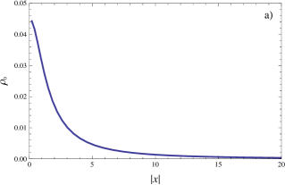
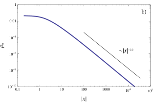
Figure 1: The minimizer $\rho_{0}$ in Theorem 3.5 for $a=1$ and $b=1$, plotted on a linear (a) and logarithmic (b) scale.

4 Preliminaries

4.1 Functional setting

Recall that the homogeneous Sobolev space $\mathring{H}^{1/2}(\mathbb{R}^{2})$ can be defined as the completion of $C^{\infty}_{c}(\mathbb{R}^{2})$ with respect to the Gagliardo’s norm

$$\|u\|_{\mathring{H}^{1/2}(\mathbb{R}^{2})}^{2}:=\frac{1}{4\pi}\iint_{\mathbb{R}^{2}\times\mathbb{R}^{2}}\frac{|u(x)-u(y)|^{2}}{|x-y|^{3}}\,\mathrm{d}^{2}x\,\mathrm{d}^{2}y.$$ (4.1)

By Plancherel’s identity (cf. (frank08, Lemma 3.1)), on $C^{\infty}_{c}(\mathbb{R}^{2})$ the $\|\cdot\|_{\mathring{H}^{1/2}(\mathbb{R}^{2})}$–norm admits an equivalent Fourier representation

$$\|u\|_{\mathring{H}^{1/2}(\mathbb{R}^{2})}^{2}=\int_{\mathbb{R}^{2}}|\,|\mathbf{k}|^{1/2}\hat{u}_{\mathbf{k}}|^{2}{\,\mathrm{d}^{2}k\over(2\pi)^{2}},\qquad\hat{u}_{\mathbf{k}}=\int_{\mathbb{R}^{2}}e^{i\mathbf{k}\cdot x}u(x)\,\mathrm{d}^{2}x,$$ (4.2)

which suggests the notation

$$\|u\|_{\mathring{H}^{1/2}(\mathbb{R}^{2})}^{2}=:\int_{\mathbb{R}^{2}}|\nabla^{\frac{1}{2}}u(x)|^{2}\,\mathrm{d}^{2}x,$$ (4.3)

which we often use in this paper. By the fractional Sobolev inequality (Lieb-Loss, Theorem 8.4), (palatucci12, Theorem 6.5),

$$\|u\|_{\mathring{H}^{1/2}(\mathbb{R}^{2})}^{2}\geq\sqrt{\pi}\,\|u\|_{L^{4}(\mathbb{R}^{2})}^{2},\qquad\forall u\in C^{\infty}_{c}(\mathbb{R}^{2}).$$ (4.4)

In particular, the space $\mathring{H}^{1/2}(\mathbb{R}^{2})$ is a well-defined space of functions and

$$\mathring{H}^{1/2}(\mathbb{R}^{2})\subset L^{4}(\mathbb{R}^{2}).$$ (4.5)

The space $\mathring{H}^{1/2}(\mathbb{R}^{2})$ is also a Hilbert space, with the scalar product associated to (4.1) given by

$$\langle u,v\rangle_{\mathring{H}^{1/2}(\mathbb{R}^{2})}:=\frac{1}{4\pi}\iint_{\mathbb{R}^{2}\times\mathbb{R}^{2}}\frac{(u(x)-u(y))(v(x)-v(y))}{|x-y|^{3}}\,\mathrm{d}^{2}x\,\mathrm{d}^{2}y.$$ (4.6)

The dual space to $\mathring{H}^{1/2}(\mathbb{R}^{2})$ is denoted $\mathring{H}^{-1/2}(\mathbb{R}^{2})$. According to the Riesz representation theorem, for every $F\in\mathring{H}^{-1/2}(\mathbb{R}^{2})$ there exists a uniquely defined potential $v\in\mathring{H}^{1/2}(\mathbb{R}^{2})$ such that

$$\langle v,\varphi\rangle_{\mathring{H}^{1/2}(\mathbb{R}^{2})}=\langle F,\varphi\rangle\qquad\forall\varphi\in\mathring{H}^{1/2}(\mathbb{R}^{2}),$$ (4.7)

where $\langle F,\cdot\rangle:\mathring{H}^{1/2}(\mathbb{R}^{2})\to\mathbb{R}$ denotes the bounded linear functional generated by $F$. Moreover,

$$\|v\|_{\mathring{H}^{1/2}(\mathbb{R}^{2})}=\|F\|_{\mathring{H}^{-1/2}(\mathbb{R}^{2})},$$ (4.8)

so the duality (4.7) is an isometry. The potential $v\in\mathring{H}^{1/2}(\mathbb{R}^{2})$ satisfying (4.7) is interpreted as the weak solution of the linear equation

$$(-\Delta)^{1/2}v=F\qquad\text{in $\mathbb{R}^{2}$}.$$ (4.9)

Recall that for functions $u\in C^{\infty}(\mathbb{R}^{2})\cap L^{1}(\mathbb{R}^{2},(1+|x|)^{-3}\,\mathrm{d}^{2}x)$, the fractional Laplacian $(-\Delta)^{1/2}$ can be defined as

$$(-\Delta)^{1/2}u(x)=\frac{1}{4\pi}\int_{\mathbb{R}^{2}}\frac{2u(x)-u(x+y)-u(x-y)}{|y|^{3}}\,\mathrm{d}^{2}y\qquad(x\in\mathbb{R}^{2}).$$ (4.10)

Note that the second order Taylor expansion of function $u$ yields that the strong singularity of the integrand at the origin is removed, and (4.10) can be understood as a converging Lebesgue integral, see (palatucci12, Lemma 3.2). Of course, the weighted second order differential quotient in (4.10) coincides with a more standard definition of $(-\Delta)^{1/2}$ as a pseudodifferential operator, in the sense that for all $u\in C^{\infty}_{c}(\mathbb{R}^{2})$,

$$\widehat{\left((-\Delta)^{1/2}u\right)_{\mathbf{k}}}=|\mathbf{k}|\hat{u}_{\mathbf{k}},$$ (4.11)

cf. (palatucci12, Proposition 3.3). In particular, this makes the definition of $(-\Delta)^{1/2}$ in (4.10) consistent with the notation used in (4.9).

Note that if $u\in C^{\infty}_{c}(\mathbb{R}^{2})$ then $(-\Delta)^{1/2}u\in C^{\infty}(\mathbb{R}^{2})$, but is not compactly supported and in fact,

$$(-\Delta)^{1/2}u=O(|x|^{-3})\qquad\text{as $|x|\to\infty$},$$ (4.12)

see (mazja, Lemma 1.2). In particular, this shows that the operator $(-\Delta)^{1/2}$ could be extended by duality to the weighted space $L^{1}(\mathbb{R}^{2},(1+|x|)^{-3}\,\mathrm{d}^{2}x)$, that is for $u\in L^{1}(\mathbb{R}^{2},(1+|x|)^{-3}\,\mathrm{d}^{2}x)$,

$$\langle(-\Delta)^{1/2}u,\varphi\rangle=\int_{\mathbb{R}^{2}}u(x)(-\Delta)^{1/2}\varphi(x)\,\mathrm{d}^{2}x\qquad\forall\varphi\in C^{\infty}_{c}(\mathbb{R}^{2})$$ (4.13)

and this definition agrees with (4.10) in the case $u\in C^{\infty}_{c}(\mathbb{R}^{2})$, see (Silvestre:07, p. 73). Clearly, $\mathring{H}^{1/2}(\mathbb{R}^{2})\subset L^{1}(\mathbb{R}^{2},(1+|x|)^{-3}\,\mathrm{d}^{2}x)$. In particular, this implies that for $v\in\mathring{H}^{1/2}(\mathbb{R}^{2})$,

$$\langle v,\varphi\rangle_{\mathring{H}^{1/2}(\mathbb{R}^{2})}=\int_{\mathbb{R}^{2}}v(x)(-\Delta)^{1/2}\varphi(x)\,\mathrm{d}^{2}x\qquad\forall\varphi\in C^{\infty}_{c}(\mathbb{R}^{2}).$$ (4.14)

When $f\in C^{\infty}_{c}(\mathbb{R}^{2})$, the left inverse to $(-\Delta)^{1/2}$ is represented by the Riesz potential, i.e., if $u$ is the weak solution of $(-\Delta)^{1/2}u=f$ then $u$ admits the integral representation

$$u(x)=(-\Delta)^{-1/2}f(x)=\frac{1}{2\pi}\int_{\mathbb{R}^{2}}\frac{f(y)}{|x-y|}\,\mathrm{d}^{2}y,$$ (4.15)

see (mazja, Lemma 1.3). Such integral representation could be extended to a wider class of functions and (signed) measures, cf. (mazja, Lemma 1.8, 1.11). In particular, taking $f=\delta(x)$, we obtain that $1/(2\pi|x|)$ is the fundamental solution of $(-\Delta)^{1/2}$. We emphasize, however, that not every potential of a linear functional $f\in\mathring{H}^{-1/2}(\mathbb{R}^{2})$ admits an integral representation (4.15). Similarly, not every linear functional $f\in\mathring{H}^{-1/2}(\mathbb{R}^{2})$ admits an integral representation of the norm in terms of the Coulomb energy. If $f\in L^{1}_{loc}(\mathbb{R}^{2})$ satisfies

$$\iint_{\mathbb{R}^{2}\times\mathbb{R}^{2}}\frac{|f(x)||f(y)|}{|x-y|}\,\mathrm{d}^{2}x\,\mathrm{d}^{2}y<+\infty.$$ (4.16)

then $f\in\mathring{H}^{-1/2}(\mathbb{R}^{2})$ in the sense that

$$\langle f,\varphi\rangle:=\int_{\mathbb{R}^{2}}f(x)\varphi(x)\,\mathrm{d}^{2}x$$ (4.17)

is a bounded linear functional on $\mathring{H}^{1/2}(\mathbb{R}^{2})$ and the norm of $\langle f,\cdot\rangle$ is expressed in terms of the Coulomb energy

$$\|f\|_{\mathring{H}^{-1/2}(\mathbb{R}^{2})}^{2}=\frac{1}{2\pi}\iint_{\mathbb{R}^{2}\times\mathbb{R}^{2}}\frac{f(x)f(y)}{|x-y|}\,\mathrm{d}^{2}x\,\mathrm{d}^{2}y,$$ (4.18)

see e.g. (mazja, pp. 96-97). In particular, from Sobolev inequality (4.4) we conclude by duality that

$$L^{4/3}(\mathbb{R}^{2})\subset\mathring{H}^{-1/2}(\mathbb{R}^{2})$$ (4.19)

and (4.18) is valid for every $f\in L^{4/3}(\mathbb{R}^{2})$. But at the same time, one could construct a sequence of sign–changing functions $\{f_{n}\}\subset C^{\infty}_{c}(\mathbb{R}^{2})$ such that $\{f_{n}\}$ is a Cauchy sequence in $\mathring{H}^{-1/2}(\mathbb{R}^{2})$, but $\{f_{n}\}$ does not converge a.e. to a measurable function or more generally, to a (signed) measure on $\mathbb{R}^{2}$. See armitage75; rempel76 or (landkof, Theorem 1.19), (duPlessis, p. 97) for other relevant examples which go back to H. Cartan (Cartan, Remark 13 on p. 87). Below we present a different example which involves smooth functions, rather than measures like in Cartan’s type examples.

Example 1

Define

$$u_{a}(x_{1},x_{2})=a^{1/2}\exp(-|x|^{2})\cos(ax_{1}).$$ (4.20)

Then, using Fourier transform, we can calculate that

$$\lVert u_{a}\rVert_{\mathring{H}^{-1/2}(\mathbb{R}^{2})}^{2}=\frac{\sqrt{2}}{8}\pi^{3/2}ae^{-\frac{a^{2}}{2}}\left(e^{\frac{a^{2}}{4}}I_{0}\bigl{(}\tfrac{1}{4}a^{2}\bigr{)}+1\right),$$ (4.21)

where $I_{0}(z)$ is the modified Bessel function of the first kind. Taking the limit $a\to\infty$, one gets

$$\lim_{a\to\infty}||u_{a}||_{\mathring{H}^{-1/2}(\mathbb{R}^{2})}^{2}={\pi\over 4}.$$ (4.22)

A Cauchy sequence in $\mathring{H}^{-1/2}(\mathbb{R}^{2})$ that fails to converge to a signed measure can then be constructed as

$$u_{n}(x_{1},x_{2})=\sum_{k=1}^{n}e^{k/4}\exp(-|x|^{2})\cos(e^{k}x_{1}).$$ (4.23)

Since this series is dominated in $\mathring{H}^{-1/2}(\mathbb{R}^{2})$ by a geometric series, it converges in $\mathring{H}^{-1/2}(\mathbb{R}^{2})$. But clearly it does not converge to a signed measure.

4.2 Hardy–Littlewood–Sobolev and Hölder estimates

We recall the well-known Hardy–Littlewood–Sobolev (stein70, Theorem 1 in Section V.1.2) and Hölder estimates on the Riesz potentials of functions in $L^{p}(\mathbb{R}^{2})$. Surprisingly, we were not able to find a concise reference to Hölder estimate, although the result is standard. Instead, we refer to (gatto, Theorem 5.2), where the estimate is obtained in an abstract framework of fractional integral operators.

Lemma 1

Let $f\in L^{s}(\mathbb{R}^{2})$ for some $s\in(1,2)$ and

$$v(x)=\frac{1}{2\pi}\int_{\mathbb{R}^{2}}\frac{f(y)}{|x-y|}\,\mathrm{d}^{2}y\qquad(x\in\mathbb{R}^{2}).$$ (4.24)

Then $v\in L^{t}(\mathbb{R}^{2})$ with $\frac{1}{t}=\frac{1}{s}-\frac{1}{2}$ and

$$\|v\|_{L^{t}(\mathbb{R}^{2})}\leq C\|f\|_{L^{s}(\mathbb{R}^{2})},$$ (4.25)

for some $C>0$ depending only on $s$. Furthermore, if $f\in L^{s}(\mathbb{R}^{2})\cap L^{1}(\mathbb{R}^{2},(1+|x|)^{-1}\,\mathrm{d}^{2}x)$ for some $s>2$, then $v\in L^{\infty}(\mathbb{R}^{2})\cap C^{1-{2\over s}}(\mathbb{R}^{2})$ and

$$|v(x)-v(y)|\leq C\|f\|_{L^{s}(\mathbb{R}^{2})}|x-y|^{1-{2\over s}}\qquad\forall x,y\in\mathbb{R}^{2},$$ (4.26)

for some $C>0$ depending only on $s$.

Remark 2

The assumption $f\in L^{1}(\mathbb{R}^{2},(1+|x|)^{-1}\,\mathrm{d}^{2}x)$ in the second part of the lemma is a necessary and sufficient condition which ensures that $|v(x)|<+\infty$ a.e. in $\mathbb{R}^{2}$, assuming that the operator in (4.24) is understood in the (Lebesgue) integral sense, c.f. (landkof, (1.3.10) on p. 61). Observe that by Hölder inequality all the assumptions of the second part of Lemma 1 are satisfied, if $f\in L^{s}(\mathbb{R}^{2})$ for all $s\in[s_{1},s_{2}]$ for some $1<s_{1}<2<s_{2}<\infty$.

4.3 Interior regularity

We are going to show that although $(-\Delta)^{1/2}$ is a nonlocal operator, the interior regularity of solutions of (4.9) does not depend on the behavior of the right-hand side at infinity. The proof of this basic fact can be found in (Silvestre:07, Proposition 2.22). Here, however, we give a quantitative version of the above statement.

Lemma 2

Let $f\in L^{1}_{loc}(\mathbb{R}^{2})$, let $p\geq 1$ and let $u\in L^{p}(\mathbb{R}^{2})$ be such that

$$\langle u,\varphi\rangle_{\mathring{H}^{1/2}(\mathbb{R}^{2})}=\int_{\mathbb{R}^{2}}f(x)\varphi(x)\,\mathrm{d}^{2}x\qquad\forall\varphi\in C^{\infty}_{c}(\mathbb{R}^{2}).$$ (4.27)

Assume that $f=0$ on $B_{2R}(0)$ for some $R>0$. Then $u\in C^{\infty}(\bar{B}_{R}(0))$ and for every $n\geq 0$

$$\|\nabla^{n}u\|_{L^{\infty}(B_{R}(0))}\leq CR^{-n-\frac{2}{p}}\|u\|_{L^{p}(\mathbb{R}^{2})}$$ (4.28)

for some $C>0$ depending only on $n$ and $p$.

Proof

Let $\eta_{R}(x)=\eta(|x|/R)$, where $\eta\in C^{\infty}(\mathbb{R})$ is a smooth cut-off function such that $\eta(x)=1$ for all $|x|>2$, $\eta(x)=0$ for all $|x|<\frac{3}{2}$, and $0\leq\eta\leq 1$. Given $\varphi\in C^{\infty}_{c}(\mathbb{R}^{2})$ supported on $B_{R}(0)$, let $\psi\in\mathring{H}^{1/2}(\mathbb{R}^{2})$ be a weak solution of $(-\Delta)^{1/2}\psi=\varphi$. By (4.15) we have

$$\psi(x)=\frac{1}{2\pi}\int_{\mathbb{R}^{2}}\frac{\varphi(y)}{|x-y|}\,\mathrm{d}^{2}y,$$ (4.29)

and, in particular, $\psi\in C^{\infty}(\mathbb{R}^{2})$. Then $(1-\eta_{R})\psi\in C^{\infty}_{c}(\mathbb{R}^{2})$ and is supported on $B_{2R}(0)$. Testing (4.27) with $(1-\eta_{R})\psi$ and taking into account (4.14), we obtain

$$0=\langle u,(1-\eta_{R})\psi\rangle_{\mathring{H}^{1/2}(\mathbb{R}^{2})}=\int_{\mathbb{R}^{2}}u(x)(-\Delta)^{1/2}\Big{(}(1-\eta_{R})\psi\Big{)}(x)\,\mathrm{d}^{2}x$$

$$=\int_{B_{R}(0)}u(x)\varphi(x)\,\mathrm{d}^{2}x-\int_{\mathbb{R}^{2}}u(x)(-\Delta)^{1/2}(\eta_{R}\psi)(x)\,\mathrm{d}^{2}x.$$ (4.30)

Inserting the definition of $(-\Delta)^{1/2}$ from (4.10) and changing the order of integration in the last integral in (4.3) yields

$$\int_{\mathbb{R}^{2}}u(x)(-\Delta)^{1/2}(\eta_{R}\psi)(x)\,\mathrm{d}^{2}x$$

$$=\frac{1}{8\pi^{2}}\int_{\mathbb{R}^{2}}u(x)\int_{\mathbb{R}^{2}}|y|^{-3}\int_{B_{R}(0)}\left(\frac{2\eta_{R}(x)}{|x-z|}-\frac{\eta_{R}(x+y)}{|x+y-z|}\right.$$

$$\hskip 170.00026pt-\left.\frac{\eta_{R}(x-y)}{|x-y-z|}\right)\varphi(z)\,\mathrm{d}^{2}z\,\mathrm{d}^{2}y\,\mathrm{d}^{2}x$$

$$=\frac{1}{8\pi^{2}}\int_{B_{R}(0)}\int_{\mathbb{R}^{2}}\left(\int_{\mathbb{R}^{2}}|y|^{-3}\left(\frac{2\eta_{R}(x)}{|x-z|}-\frac{\eta_{R}(x+y)}{|x+y-z|}\right.\right.$$

$$\hskip 170.00026pt-\left.\left.\frac{\eta_{R}(x-y)}{|x-y-z|}\right)\,\mathrm{d}^{2}y\right)u(x)\varphi(z)\,\mathrm{d}^{2}x\,\mathrm{d}^{2}z$$

$$=\int_{B_{R}(0)}\int_{\mathbb{R}^{2}}J_{R}(x,z)u(x)\varphi(z)\,\mathrm{d}^{2}x\,\mathrm{d}^{2}z,$$ (4.31)

where for $x\in\mathbb{R}^{2}$ and $z\in B_{R}(0)$ we introduced

$$J_{R}(x,z):=\frac{1}{8\pi^{2}}\int_{\mathbb{R}^{2}}|y|^{-3}\left(\frac{2\eta_{R}(x)}{|x-z|}-\frac{\eta_{R}(x+y)}{|x+y-z|}-\frac{\eta_{R}(x-y)}{|x-y-z|}\right)\,\mathrm{d}^{2}y.$$ (4.32)

Observe that

$$J_{R}(x,z)=(-\Delta)^{1/2}_{x}j_{R}(x,z),\qquad j_{R}(x,z):=\frac{1}{2\pi}\frac{\eta_{R}(x)}{|x-z|}.$$ (4.33)

Clearly, $j_{R}(x,z)=0$ for $x\in B_{3R/2}(0)$ and $j_{R}\in C^{\infty}(\mathbb{R}^{2}\times\bar{B}_{R}(0))$, with

$$|\nabla^{n}_{z}j_{R}(x,z)|\leq c_{n}(R+\left\lvert x-z\right\rvert)^{-(n+1)},$$ (4.34)

$$|\nabla^{2}_{x}\nabla^{n}_{z}j_{R}(x,z)|\leq c_{n}R^{-2}(R+\left\lvert x-z\right\rvert)^{-(n+1)}$$ (4.35)

for all $n\geq 0$ and some $c_{n}>0$ (unless stated otherwise, all constants in this proof depend only on $n$ and the choice of $\eta$). Then

$$\left\lvert\nabla^{n}_{z}J_{R}(x,z)\right\rvert\leq\frac{1}{8\pi^{2}}\int_{\mathbb{R}^{2}}|y|^{-3}\Big{\lvert}2\nabla^{n}_{z}j_{R}(x,z)-\nabla^{n}_{z}j_{R}(x+y,z)$$

$$\hskip 180.00027pt-\nabla^{n}_{z}j_{R}(x-y,z)\Big{\rvert}\,\mathrm{d}^{2}y$$

$$=\frac{1}{8\pi^{2}}\int_{B_{R}(0)}|y|^{-3}\Big{|}2\nabla^{n}_{z}j_{R}(x,z)-\nabla^{n}_{z}j_{R}(x+y,z)-\nabla^{n}_{z}j_{R}(x-y,z)\Big{|}\,\mathrm{d}^{2}y$$

$$\quad+\frac{1}{8\pi^{2}}\int_{\mathbb{R}^{2}\backslash B_{R}(0)}|y|^{-3}\Big{|}2\nabla^{n}_{z}j_{R}(x,z)-\nabla^{n}_{z}j_{R}(x+y,z)-\nabla^{n}_{z}j_{R}(x-y,z)\Big{|}\,\mathrm{d}^{2}y$$

$$\leq\frac{1}{8\pi^{2}}\lVert\nabla^{2}_{x}\nabla^{n}_{z}j_{R}(\cdot,z)\rVert_{L^{\infty}(\mathbb{R}^{2})}\int_{B_{R}(0)}\left\lvert y\right\rvert^{-1}\,\mathrm{d}^{2}y$$

$$\quad+\frac{1}{2\pi^{2}}\lVert\nabla^{n}_{z}j_{R}(\cdot,z)\rVert_{L^{\infty}(\mathbb{R}^{2})}\int_{\mathbb{R}^{2}\backslash B_{R}(0)}|y|^{-3}\,\mathrm{d}^{2}y$$

$$\leq C_{n}R^{-n-2},$$ (4.36)

for some $C_{n}>0$. In particular, for any $x\in\mathbb{R}^{2}$, $J_{R}(x,\cdot)\in C^{\infty}(\bar{B}_{R}(0))$.

We next prove that for some $c_{n}>0$ we have

$$|\nabla_{z}^{n}J_{R}(x,z)|\leq\frac{c_{n}}{R^{n-1}(R^{3}+|x|^{3})}\qquad\forall x\in\mathbb{R}^{2},\quad\forall z\in\bar{B}_{R}(0).$$ (4.37)

For $\left\lvert x\right\rvert\leq 4R$, the estimate follows from (4.3). Now assume $|x|\geq 4R$. Then $\eta_{R}(x)=1$, and since $1/(2\pi\left\lvert x\right\rvert)$ is the fundamental solution for $(-\Delta)^{1/2}$, we have for $\left\lvert z\right\rvert\leq R$

$$\frac{1}{8\pi^{2}}\int_{\mathbb{R}^{2}}|y|^{-3}\left(\frac{2}{|x-z|}-\frac{1}{|x+y-z|}-\frac{1}{|x-y-z|}\right)\,\mathrm{d}^{2}y=0.$$ (4.38)

Using this fact we can rewrite

$$J_{R}(x,z) =\frac{1}{8\pi^{2}}\int_{\mathbb{R}^{2}}\frac{1-\eta_{R}(x-y)}{|x-y-z|}|y|^{-3}\,\mathrm{d}^{2}y+\frac{1}{8\pi^{2}}\int_{\mathbb{R}^{2}}\frac{1-\eta_{R}(x+y)}{|x+y-z|}|y|^{-3}\,\mathrm{d}^{2}y$$

$$=\frac{1}{8\pi^{2}}\int_{\mathbb{R}^{2}}\frac{1}{|y-z|}\left(\frac{1-\eta_{R}(y)}{\left\lvert x-y\right\rvert^{3}}+\frac{1-\eta_{R}(y)}{\left\lvert x+y\right\rvert^{3}}\right)\,\mathrm{d}^{2}y$$

$$=:\frac{1}{8\pi^{2}}\int_{\mathbb{R}^{2}}\frac{1}{|y-z|}h_{R}(x,y)\,\mathrm{d}^{2}y.$$ (4.39)

Notice that for fixed $x$ with $\left\lvert x\right\rvert\geq 4R$, $h_{R}(x,\cdot)\in C^{\infty}_{c}(\mathbb{R}^{2})$ and its support is contained in $B_{2R}(0)$. Therefore,

$$\left\lvert\nabla^{n}_{z}J_{R}(x,z)\right\rvert \leq\frac{1}{8\pi^{2}}\int_{B_{2R}(0)}\frac{1}{\left\lvert y-z\right\rvert}\left\lvert\nabla^{n}_{y}h_{R}(x,y)\right\rvert\,\mathrm{d}^{2}y.$$ (4.40)

For $y\in B_{2R(0)}$ and $\left\lvert x\right\rvert\geq 4R$, we have the estimate $\left\lvert\nabla^{n}_{y}h_{R}(x,y)\right\rvert\leq C_{n}R^{-n}\left\lvert x\right\rvert^{-3}$ for some $C_{n}>0$. Therefore,

$$|\nabla_{z}^{n}J_{R}(x,z)|\leq\frac{C_{n}}{R^{n}|x|^{3}}\int_{B_{2R}(0)}\frac{1}{|y-z|}\,\mathrm{d}^{2}y\leq\frac{C_{n}^{\prime}}{R^{n-1}|x|^{3}},$$ (4.41)

for some $C_{n}^{\prime}>0$.

Finally, taking into account (4.3), we conclude that for almost every $z\in\bar{B}_{R}(0)$ we have

$$u(z)=\int_{\mathbb{R}^{2}}J_{R}(x,z)u(x)\,\mathrm{d}^{2}x,$$ (4.42)

and, since (4.37) leads to $\|\nabla_{z}^{n}J_{R}(\cdot,z)\|_{L^{p\over p-1}(\mathbb{R}^{2})}\leq CR^{-n-2/p}$ for some $C>0$ depending only on $n$, $p$ and the choice of $\eta$, the statement of the lemma follows by Hölder inequality. ∎

5 Variational setting

5.1 A representation of the energy functional

Recall that for a given $\rho\in\mathcal{A}_{\bar{\rho}}$ we define $u$ by

$$u:=\operatorname{sgn}(\rho)\sqrt{|\rho|}-\operatorname{sgn}(\bar{\rho})\sqrt{|\bar{\rho}|}$$ (5.1)

and set $\bar{u}:=\sqrt{\left\lvert\bar{\rho}\right\rvert}\operatorname{sgn}{\bar{\rho}}$. Then $u\in\mathring{H}^{1/2}(\mathbb{R}^{2})$ in view of the definition of $\mathcal{A}_{\bar{\rho}}$. Since $\operatorname{sgn}(\rho)\sqrt{|\rho|}=u+\bar{u}$, we can define

$$\int_{\mathbb{R}^{2}}\big{|}\nabla^{\frac{1}{2}}\bigl{(}\sqrt{\left\lvert\rho(x)\right\rvert}\operatorname{sgn}(\rho(x))\bigr{)}\big{|}^{2}\,\mathrm{d}^{2}x:=\\ \frac{1}{4\pi}\iint_{\mathbb{R}^{2}\times\mathbb{R}^{2}}\frac{|(u(x)+\bar{u})-(u(y)+\bar{u})|^{2}}{|x-y|^{3}}\,\mathrm{d}^{2}x\,\mathrm{d}^{2}y=\|u\|_{\mathring{H}^{1/2}(\mathbb{R}^{2})}^{2},$$ (5.2)

which justifies and clarifies the notation used in Sections 1–3 of the paper.

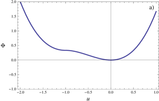
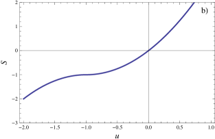
Figure 2: (a) Plot of $\Phi(u)$ and (b) plot of $S(u)$ for $\bar{u}=1$.

Throughout the rest of the paper we assume, without loss of generality, that $\bar{\rho}\geq 0$, and, hence, $\bar{u}\geq 0$ (see (3.1)). Denote

$$S(u):=|u+\bar{u}|(u+\bar{u})-|\bar{u}|\bar{u}=\begin{cases}2\bar{u}u+u^{2},&u\geq-\bar{u},\\ -u^{2}-2\bar{u}u-2\bar{u}^{2},&u<-\bar{u},\end{cases}$$ (5.3)

and

$$\Phi(u):=\frac{2}{3}(|u+\bar{u}|^{3}-|\bar{u}|^{3})-\bar{u}S(u)=\left\{\begin{array}[]{ll}\hskip 7.5pt\frac{2}{3}u^{3}+\bar{u}u^{2},&u\geq-\bar{u},\vskip 3.0pt plus 1.0pt minus 1.0pt\\ -\frac{2}{3}u^{3}-\bar{u}u^{2}+\frac{2}{3}\bar{u}^{3},&u<-\bar{u}.\end{array}\right.$$ (5.6)

The graphs of $\Phi(u)$ and $S(u)$ for $\bar{u}=1$ are presented in Fig. 2. Clearly $S,\Phi\in C^{1}(\mathbb{R})$ and both functions are smooth functions of $u\in\mathbb{R}$ except at $u=-\bar{u}$. Moreover

$$c(\bar{u}|u|^{2}+|u|^{3})\leq\Phi(u)\leq C(\bar{u}|u|^{2}+|u|^{3})\qquad(u\in\mathbb{R}),$$ (5.7)

$$c(\bar{u}|u|+|u|^{2})\leq S(u)\operatorname{sgn}(u)\leq C(\bar{u}|u|+|u|^{2})\qquad(u\in\mathbb{R}),$$ (5.8)

for some universal $C>c>0$. Therefore, for $u\in C^{\infty}_{c}(\mathbb{R}^{2})$, the energy $E(u)$ can be written as (with a slight abuse of notation, we use the same letter to denote both the energy as a function of $\rho$ and that as a function of $u$ in the rest of the paper)

$$E(u)=a\|u\|_{\mathring{H}^{1/2}(\mathbb{R}^{2})}^{2}+\int_{\mathbb{R}^{2}}\Phi(u(x))\,\mathrm{d}^{2}x\\ +\int_{\mathbb{R}^{2}}V(x)S(u(x))\,\mathrm{d}^{2}x+\frac{b}{2}\iint_{\mathbb{R}^{2}\times\mathbb{R}^{2}}\frac{S(u(x))S(u(y))}{\left\lvert x-y\right\rvert}\,\mathrm{d}^{2}x\,\mathrm{d}^{2}y.$$ (5.9)

Given $u\in\mathring{H}^{1/2}(\mathbb{R}^{2})$, (4.5) and (5.8) imply that $S(u)\in L^{2}_{loc}(\mathbb{R}^{2})$. Then for all $\varphi\in C^{\infty}_{c}(\mathbb{R}^{2})$ we can define

$$\langle S(u),\varphi\rangle:=\int_{\mathbb{R}^{2}}S(u(x))\varphi(x)\,\mathrm{d}^{2}x.$$ (5.10)

We say $S(u)\in\mathring{H}^{-1/2}(\mathbb{R}^{2})$, if the linear functional $\langle S(u),\cdot\rangle$ defined in (5.10) is bounded by a multiple of $\|\varphi\|_{\mathring{H}^{1/2}(\mathbb{R}^{2})}$. In that case $\langle S(u),\cdot\rangle$ is understood as the unique continuous extension of (5.10) to $\mathring{H}^{1/2}(\mathbb{R}^{2})$. Note that $S(u)\in\mathring{H}^{-1/2}(\mathbb{R}^{2})$ does not necessarily imply that $S(u)w\in L^{1}(\mathbb{R}^{2})$ for every $w\in\mathring{H}^{1/2}(\mathbb{R}^{2})$. In other words, $\langle S(u),\cdot\rangle$ does not always admit an integral representation on $\mathring{H}^{1/2}(\mathbb{R}^{2})$, as observed by Brezis and Browder in brezis79 in the context of $H^{1}(\mathbb{R}^{N})$.

5.2 Class $\mathcal{H}$

Introduce the class

$$\mathcal{H}:=\Bigl{\{}u\in\mathring{H}^{1/2}(\mathbb{R}^{2}):S(u)\in\mathring{H}^{-1/2}(\mathbb{R}^{2})\Bigr{\}}.$$ (5.11)

As discussed in Section 5.1, this is an equivalent way of writing the class $\mathcal{A}_{\bar{\rho}}$. Given $u\in\mathcal{H}$, Riesz’s representation theorem uniquely defines a potential $U_{S(u)}\in\mathring{H}^{1/2}(\mathbb{R}^{2})$ such that

$$\langle{U}_{S(u)},\varphi\rangle_{\mathring{H}^{1/2}(\mathbb{R}^{2})}=\langle S(u),\varphi\rangle\qquad\forall\varphi\in\mathring{H}^{1/2}(\mathbb{R}^{2}).$$ (5.12)

In particular, from the Sobolev embedding (4.5) combined with (5.7) we obtain the following inclusions:

$$\{u\in\mathcal{H}\ :\ E(u)<+\infty\}\subset L^{4}(\mathbb{R}^{2})\cap L^{2}(\mathbb{R}^{2})\qquad\text{if $\bar{u}\neq 0$,}$$ (5.13)

$$\{u\in\mathcal{H}\ :\ E(u)<+\infty\}\subset L^{4}(\mathbb{R}^{2})\cap L^{3}(\mathbb{R}^{2})\qquad\text{if $\bar{u}=0$}.$$ (5.14)

Remark 3

In fact, using a fractional extension of the Brezis-Browder argument in brezis79, one can establish stronger inclusions:

$$\mathcal{H}\subset L^{4}(\mathbb{R}^{2})\cap L^{2}(\mathbb{R}^{2})\qquad\text{if $\bar{u}\neq 0$,}$$ (5.15)

$$\mathcal{H}\subset L^{4}(\mathbb{R}^{2})\cap L^{3}(\mathbb{R}^{2})\qquad\text{if $\bar{u}=0$}.$$ (5.16)

We refer to the forthcoming work lmm2 for the details. Moreover, these inclusions are, in some sense optimal. To see the optimality of (5.15), choose $u\in C^{\infty}_{c}(B_{1}(0))$, a vector $e\in\mathbb{R}^{2}$ with $|e|=1$ and for $N\in\mathbb{N}$ let

$$u_{N}(x):=\frac{1}{\sqrt{N}}\sum_{k=1}^{N}u\big{(}x+k\exp(N)e\big{)}.$$ (5.17)

It is standard to check (cf. (4.12) for the $\mathring{H}^{1/2}$–term and (ruiz10, p. 363) for the Coulomb term) that

$$\|u_{N}\|_{\mathring{H}^{1/2}(\mathbb{R}^{2})}\simeq\|S(u_{N})\|_{\mathring{H}^{-1/2}(\mathbb{R}^{2})}\simeq C,$$ (5.18)

while

$$\|u_{N}\|_{L^{p}(\mathbb{R}^{2})}=O(N^{\frac{1}{p}-\frac{1}{2}}).$$ (5.19)

We conclude that the sequence $\{u_{N}\}$ is not bounded in $L^{p}(\mathbb{R}^{2})$ for any $p<2$. To check the optimality of (5.16), instead of (5.17) one can use an appropriately rescaled family of functions $u_{N}$, similar to those in (ruiz10, Proof of Theorem 1.5).

6 Proof of Theorems 3.1 and 3.3

6.1 Existence of a minimizer

If $V\in\mathring{H}^{1/2}(\mathbb{R}^{2})$ then we can rewrite $E$ in terms of $u$ and the associated potential ${U}_{S(u)}$ as

$$E(u)=a\|u\|_{\mathring{H}^{1/2}(\mathbb{R}^{2})}^{2}+\int_{\mathbb{R}^{2}}\Phi(u(x))\,\mathrm{d}^{2}x+\langle V,{U}_{S(u)}\rangle_{\mathring{H}^{1/2}(\mathbb{R}^{2})}+\frac{b}{2}\|{U}_{S(u)}\|_{\mathring{H}^{1/2}(\mathbb{R}^{2})}^{2}.$$ (6.1)

In particular, it is easy to see that

$$-\frac{1}{2b}\|V\|_{\mathring{H}^{1/2}(\mathbb{R}^{2})}^{2}\leq\inf_{u\in\mathcal{H}}E(u)\leq 0.$$ (6.2)

We are going to prove that $E$ attains a minimizer on $\mathcal{H}$.

Proposition 1

If $V\in\mathring{H}^{1/2}(\mathbb{R}^{2})$ then there exists $u_{0}\in\mathcal{H}$ such that $E(u_{0})=\inf_{u\in\mathcal{H}}E(u)$.