Asymptotic charged BTZ black hole solutions

Abstract

The well-known $(2+1)$-dimensional Reissner-Nordström (BTZ) black hole can be generalized to three dimensional Einstein-nonlinear electromagnetic field, motivated from obtaining a finite value for the self-energy of a pointlike charge. Considering three types of nonlinear electromagnetic fields coupled with Einstein gravity, we derive three kinds of black hole solutions which their asymptotic properties are the same as charged BTZ solution. In addition, we calculate conserved and thermodynamic quantities of the solutions and show that they satisfy the first law of thermodynamics. Finally, we perform a stability analysis in the canonical ensemble and show that the black holes are stable in the whole phase space.

I Introduction

Nonlinear field theories are of interest to different branches of mathematical physics because most physical systems are inherently nonlinear in nature. Nonlinear action of Abelian gauge theories have been considered in the context of superstring theory. In fact, it has shown that Fradkin85 all order loop corrections to gravity may be considered as a Born-Infeld (BI) type Lagrangian BI . Also, the dynamics of D-branes and some soliton solutions of supergravity are governed by the BI action Leigh89 . The first attempt to relate the nonlinear electrodynamics (NLEDs) and gravity was made by Hoffmann Hoffmann . Considering NLEDs coupled to the gravitational field (with or without scalar field) may lead to black hole solutions with interesting properties BIpaper ; PMIpaper ; Ayon98 ; Oliveira94 ; Soleng .

In addition to the nonlinear BI, other types of NLEDs have been studied in a number of papers PMIpaper ; Soleng . It is known that the NLEDs proposed by Born and Infeld had the aim of obtaining a finite value for the self-energy of a point-like charge. So in this paper, we consider three kinds of BI-type fields with the following motivations:

First, modifying the linear Maxwell theory to NLED theory may eliminate the problem of divergency in electromagnetic field.

Second, it is notable that one can find regular black hole solutions of the Einstein field equations coupled to a suitable NLEDs Oliv94 ; Soleng ; Palatnik98 ; Ayon46 ; Ayon84 ; Ayon99 . Also, an interesting property which is common to all the NLED models is the fact that these models satisfy the zeroth and first laws of black hole mechanics Rasheed97 .

Third, it is also remarkable that, BI-type theories are singled out among the classes of NLEDs by their special properties such as the absence of shock waves, birefringence phenomena Boillat and enjoying an electric-magnetic duality GibRash .

Fourth, the appropriate world-volume dynamics on a curved $D3$-brane may provide a plausible frame-work at Planck scale by incorporating the Einstein-NLEDs. At this point of time, elimination of strong intrinsic curvature in the regime by the strong nonlinearity in the $U(1)$ gauge theory is remarkable Gopakumar ; Ayon99 ; Tamaki2000 ; Kar05 .

Fifth, from the point of view of AdS/CFT correspondence in hydrodynamic models, it has been shown that, unlike gravitational correction, higher-derivative terms for Abelian fields in the form of NLED do not affect this ratio Brigante ; Kovtun ; CaiJHEP08 ; GeJHEP08 . In addition, in applications of the AdS/CFT correspondence to superconductivity, NLED theories make crucial effects on the condensation Jing10 as well as the critical temperature of the superconductor and its energy gap Gregory09 ; Pan10 .

Sixth, it has been shown that Salim55 ; Salim25 the effects of NLED become important when we investigate super-strongly magnetized compact objects, such as pulsars, neutron stars, magnetars and strange quark magnetars. In addition, it has proved that Salim55 if one consider a NLED to incorporate into the photon dynamics, Gravitational Redshift depends on the magnetic field pervading the pulsar (while the Gravitational Redshift is independent of any background magnetic field in general relativity). Also, since the Gravitational Redshift of magnetized compact objects is connected to the mass–radius relation of the objects, it is important to note that NLED affects on the mass–radius relation of the objects.

Motivated by the recent results mentioned above, we study black hole solutions in Einstein gravity with negative cosmological constant coupled to NLED theory. Considering these nonlinear fields in $(2+1)$-dimensional spacetime, with asymptotic BTZ (Banados–Teitelboim–Zanelli) behavior, help us to find a simple mechanism for analyzing the properties of the solutions.

Physicists believe that one of the great achievements in gravity is discovery of the $(2+1)$-dimensional BTZ black hole solutions BTZ1 ; BTZ2 ; BTZ3 . In fact, BTZ black holes provide a simplified model to investigate and find some conceptual issues such as black hole thermodynamics Carlip95 ; Ashtekar02 ; Sarkar06 , quantum gravity, string and gauge theory and specially, in the context of the AdS/CFT conjecture Witten98 ; Carlip05 . Furthermore, BTZ solutions perform a central role to improve our perception of gravitational interaction in low dimensional spacetime Witten07 . Generalization of BTZ black hole and its properties to higher dimensions and also its near-horizon solutions have been studied in Thermodynamics ; Saida99 ; Cadoni08 ; Larranaga10 ; Hyun97 ; Sfetsos98 ; Canfora10 ; Claessens09 ; BTZlike .

Since in this paper, we consider three classes of the Einstein-NLED field and expect to obtain asymptotic BTZ black hole, we want to discuss about two significant properties of charged BTZ solutions. First, it is notable that for $(2+1)$-dimensional charged BTZ solutions, $A_{t}$ and the electromagnetic field are proportional to $\ln r$ and $r^{-1}$, respectively. Second, the charge term of the laps function in horizon flat $(2+1)$-dimensional BTZ solutions, is a logarithmic function of $r$.

Organization of the paper is as follows: at first, we give a brief review of the field equations of Einstein gravity sourced by the NLED field. Then we consider three dimensional spacetime and find relative solutions. After that we investigate their properties, especially singularity and asymptotic behavior of them. Then, we obtain conserved and thermodynamic quantities of the black holes, in which satisfy the first law of thermodynamics. Also, we analyze the local stability in canonical ensemble and at last we confirm that obtained solutions are asymptotic BTZ. We finish our paper with some conclusions.

II $(2+1)$-dimensional black holes with NLED field

The $(2+1)$-dimensional action of Einstein gravity with NLED field in the presence of cosmological constant is given by

$$I_{G}=-\frac{1}{16\pi}\int_{\mathcal{M}}d^{3}x\sqrt{-g}\left[R-2\Lambda+L(\mathcal{F})\right]-\frac{1}{8\pi}\int_{\partial\mathcal{M}}d^{2}x\sqrt{-\gamma}K,$$ (1)

where ${R}$ is the Ricci scalar, $\Lambda$ refers to the negative cosmological constant which in general is equal to $-1/l^{2}$ for asymptotically anti-deSitter solutions, in which $l$ is a scale length factor. In Eq. (1), $L(\mathcal{F})$ is the Lagrangian of NLED field. Here, we consider three classes of Born-Infeld-like NLED fields, namely Born-Infeld nonlinear electromagnetic (BINEF), Exponential form of nonlinear electromagnetic field (ENEF) and Logarithmic form of nonlinear electromagnetic field (LNEF) in which their Lagrangians are

$$L(\mathcal{F})=\left\{\begin{array}[]{ll}4\beta^{2}\left(1-\sqrt{1+\frac{\mathcal{F}}{2\beta^{2}}}\right),&\text{BINEF}\\ \beta^{2}\left(\exp(-\frac{\mathcal{F}}{\beta^{2}})-1\right),&\text{ENEF}\\ -8\beta^{2}\ln\left(1+\frac{\mathcal{F}}{8\beta^{2}}\right),&\text{LNEF}\end{array}\right..$$ (2)

In this equation, $\beta$ is called the nonlinearity parameter, the Maxwell invariant $\mathcal{F}=F_{\mu\nu}F^{\mu\nu}$ in which $F_{\mu\nu}=\partial_{\mu}A_{\nu}-\partial_{\nu}A_{\mu}$ is the electromagnetic field tensor and $A_{\mu}$ is the gauge potential.

It is natural to expect that the nonlinear electromagnetic field appears as an effective theory of string/M—theory. For instance, one of the subgroup of the $E_{8}\times E_{8}$ or $SO(32)$ gauge group is $U(1)$. Ignoring all other gauge fields leaves us with the effective quartic order of $U(1)$ Lagrangian, $(F_{\mu\nu}F^{\mu\nu})^{2}$ Liu26 ; Gross87 ; Bergshoeff ; Chemissany07 . In addition, Natsuume Natsuume considered the next order correction terms in the heterotic string effective action of a magnetically-charged black hole GHS and obtained the $(F_{\mu\nu}F^{\mu\nu})^{2}$ term as a subset of all possible $\alpha$ corrections to the bosonic sector of supergravity, which is the same order as the Gauss-Bonnet term Liu26

$$L_{cor}=\alpha\left[a\left(R_{\mu\nu\rho\sigma}R^{\mu\nu\rho\sigma}-4R_{\mu\nu}R^{\mu\nu}+R^{2}\right)+b\left(F_{\mu\nu}F^{\mu\nu}\right)^{2}\right].$$ (3)

Furthermore, calculating one-loop approximation of QED, it has shown that Ritz the effective Lagrangian is given by

$$L_{eff}=c\left(F_{\mu\nu}F^{\mu\nu}\right)+d\left(F_{\mu\nu}F^{\mu\nu}\right)^{2}.$$ (4)

Euler and Heisenberg have shown that the correction contain logarithmic form in the electromagnetic field strength appear in the calculation of exact $1$-loop corrections for electrons in a uniform electromagnetic field background Heisenberg , which is description of vacuum polarization effects. So, these corrections are a kind of effective actions in quantum electrodynamics.

Furthermore, logarithmic form of the electrodynamic Lagrangians, like BI electrodynamics, removes divergences in the electric field. Although the exponential form of BI-like NLED does not cancel the divergency of electric field at $r=0$, but its singularity is too much weaker than in, e.g., Einstein-Maxwell gravity.

From the cosmological point of view, these BI-like NLEDs have also been used to explain an equation of state of radiation for inflation Altshuler . As an example of a BI-like Lagrangian with a logarithmic term, four dimensional asymptotically flat solutions of Einstein gravity was discussed in Soleng . Expanding $L(\mathcal{F})$’s for large values of $\beta$, one can write

$$\left.L(\mathcal{F})\right|_{\text{Large }\beta}=\left\{\begin{array}[]{ll}-\mathcal{F}+\frac{\mathcal{F}^{2}}{8\beta^{2}}-\frac{\mathcal{F}^{3}}{32\beta^{4}}+\frac{5\mathcal{F}^{4}}{512\beta^{6}}+O\left(\frac{1}{\beta^{8}}\right),&\text{BINEF}\\ -\mathcal{F}+\frac{\mathcal{F}^{2}}{2\beta^{2}}-\frac{\mathcal{F}^{3}}{6\beta^{4}}+\frac{\mathcal{F}^{4}}{24\beta^{6}}+O\left(\frac{1}{\beta^{8}}\right),&\text{ENEF}\\ -\mathcal{F}+\frac{\mathcal{F}^{2}}{16\beta^{2}}-\frac{\mathcal{F}^{3}}{192\beta^{4}}+\frac{\mathcal{F}^{4}}{2048\beta^{6}}+O\left(\frac{1}{\beta^{8}}\right),&\text{LNEF}\end{array}\right.$$ (5)

which confirm that $L(\mathcal{F})$’s reduce to the standard Maxwell form $L(\mathcal{F})=-\mathcal{F}$, for $\beta\longrightarrow\infty$ and also the leading first correction of Maxwell theory has $\left(F_{\mu\nu}F^{\mu\nu}\right)^{2}$ form.

Furthermore, we should note that the second integral in Eq. (1) is the Gibbons-Hawking surface term GibHaw which is chosen such that the variational principle is well defined. The factor $K$ is the trace of the extrinsic curvature $K_{ab}$ of any boundary ${\partial\mathcal{M}}$ of the manifold ${\mathcal{M}}$, with induced metric $\gamma_{ab}$. Although three dimensional solution of Einstein-BI gravity has been investigated before BIBTZ , but we present it again with two motivations: firstly, one can confirm that our BI solution is more compact and we discuss about the geometry of BI black hole and its horizon precisely, and secondly, in order to compare the solutions of the exponential and logarithmic Lagrangian with BI solution, we need to present BI solution here.

Varying the action (1) with respect to the gravitational field $g_{\mu\nu}$ and the gauge field $A_{\mu}$, the field equations are obtained as

$$R_{\mu\nu}-\frac{1}{2}g_{\mu\nu}\left(R-2\Lambda\right)=\alpha T_{\mu\nu},$$ (6)

$$\partial_{\mu}\left(\sqrt{-g}L_{\mathcal{F}}F^{\mu\nu}\right)=0,$$ (7)

where

$$T_{\mu\nu}=\frac{1}{2}g_{\mu\nu}L(\mathcal{F})-2F_{\mu\lambda}F_{\nu}^{\;\lambda}L_{\mathcal{F}},$$ (8)

and $L_{\mathcal{F}}=\frac{dL(\mathcal{F})}{d\mathcal{F}}$. Our main aim here is to obtain charged static black hole solutions of the field equations (6) - (8) and investigate their properties. We assume $(2+1)$-dimensional metric has the following form

$$ds^{2}=-f(r)dt^{2}+\frac{dr^{2}}{f(r)}+r^{2}d\theta^{2}$$ (9)

Using the gauge potential ansatz $A_{\mu}=h(r)\delta_{\mu}^{0}$ in the NLED fields equation (7) leads to the following differential equations

$$\begin{array}[]{rr}rh^{\prime\prime}(r)+h^{\prime}(r)\left[1-\left(\frac{h^{\prime}(r)}{\beta}\right)^{2}\right]=0,&\text{BINEF}\vspace{0.1cm}\\ r\left[1+\frac{4}{\beta^{2}}h^{\prime}(r)\right]h^{\prime\prime}(r)+h^{\prime}(r)=0,&\text{ENEF}\vspace{0.1cm}\\ r\left[1+\left(\frac{h^{\prime}(r)}{2\beta}\right)^{2}\right]h^{\prime\prime}(r)+h^{\prime}(r)\left[1-\left(\frac{h^{\prime}(r)}{2\beta}\right)^{2}\right]=0,&\text{LNEF}\end{array},$$ (10)

with the following solutions

$$h(r)=\frac{q}{2}\times\left\{\begin{array}[]{ll}2\ln\left[\frac{r}{2l}\left(1+\Gamma\right)\right],&\text{BINEF}\vspace{0.1cm}\\ \frac{\beta r\sqrt{L_{W}}}{q}+{Ei}\left(1,\frac{L_{W}}{2}\right)+\ln\left(\frac{2q^{2}}{l^{2}\beta^{2}}\right)+\gamma-2,&\text{ENEF}\vspace{0.1cm}\\ 2\ln\left[\frac{r}{2l}\left(1+\Gamma\right)\right]-\frac{2r^{2}\beta^{2}}{q^{2}}\left(1-\Gamma\right)-1,&\text{LNEF}\end{array}\right.,$$ (11)

where $\Gamma=\sqrt{1+\frac{q^{2}}{r^{2}\beta^{2}}}$, $q$ is an integration constant which is related to the electric charge of the black hole. In addition, $L_{W}=LambertW(\frac{4q^{2}}{r^{2}\beta^{2}})$ which satisfies $LambertW(x)\exp\left[LambertW(x)\right]=x$, $\gamma=\gamma(0)\simeq 0.57722$ and the special function ${Ei}\left(1,x\right)=\int\limits_{1}^{\infty}\frac{e^{-xz}}{z}dz$ (for more details, see Lambert ).

It is easy to show that the non-vanishing components of the electromagnetic field tensor can be written in the following form

$$F_{tr}=\frac{q}{r}\times\left\{\begin{array}[]{ll}\Gamma^{-1},&\text{BINEF}\\ \frac{r\beta\sqrt{L_{W}}}{2q},&\text{ENEF}\\ \frac{2\beta^{2}r^{2}}{q^{2}}\left(\Gamma-1\right),&\text{LNEF}\end{array}\right..$$ (12)

Considering Fig. 1, it is interesting to note that all three types of the mentioned electromagnetic fields have finite values near the origin and they vanish at large values of $r$, as it should be. In addition, this figure shows that the effect of nonlinearity parameter, $\beta$, on the strength of electromagnetic fields is more considerable for small values of distances. Furthermore, Fig. 2 shows that the mentioned NLED fields have different values for the fixed parameters and one may think they have finite values at the origin ($r\rightarrow 0$), but it is interesting to note that $F^{ENEF}_{tr}$ diverges at $r=0$ (see table A for more details).

$r=$	$10^{-2}$	$10^{-10}$	$10^{-20}$	$10^{-50}$	$10^{-100}$	$10^{-1000}$	$r\longrightarrow 0$
$F_{tr}^{BINEF}$	$4.993$	$5.000$	$5.000$	$5.000$	$5.000$	$5.000$	$5.000$
$F_{tr}^{ENEF}$	$5.941$	$15.91$	$23.16$	$37.33$	$53.18$	$169.5$	$\infty$
$F_{tr}^{LNEF}$	$9.512$	$9.999$	$10.00$	$10.00$	$10.00$	$10.00$	$10.00$
$F_{tr}^{BTZ}$	$10^{2}$	$10^{10}$	$10^{20}$	$10^{50}$	$10^{100}$	$10^{1000}$	$\infty$

Table A: $F_{tr}$ for $\beta=5$, $q=1$, $l=1$ and small values of $r$.

$\begin{array}[]{ccc}\epsfbox{EBI.eps}&\epsfbox{Eexp.eps}&\epsfbox{Elog.eps}\end{array}$

Figure 1: $F_{tr}$ versus $r$ for $l=1$, $q=1$ and $\beta=5$ (Bold line), $\beta=10$ (solid line), $\beta=15$ (dashed line) and $\beta\longrightarrow\infty$ (BTZ solution) (dotted line). ”BINEF (left), ENEF (middle) and LNEF (right)”

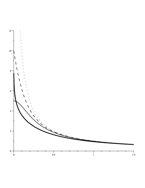
Figure 2: $F_{tr}$ versus $r$ in ENEF (Bold line), BINEF (solid line), LNEF (dashed line) and BTZ solution (dotted line) for $l=1$, $q=1$ and $\beta=5$.

To find the metric function $f(r)$, one may use any components of Eq. (6). Considering the function $h(r)$, the nontrivial independent components of the field equation, (6), are

$$\begin{array}[]{rr}\left.\begin{array}[]{r}f^{\prime}(r)-\frac{2r}{l^{2}}-4r\beta^{2}\left(1-\Gamma\right)=0,\\ f^{\prime\prime}(r)-\frac{2}{l^{2}}-4\beta^{2}\left(1-\Gamma^{-1}\right)=0.\end{array}\right\},&\text{BINEF}\vspace{0.2cm}\\ \left.\begin{array}[]{r}f^{\prime}(r)-\frac{2r}{l^{2}}+r\beta^{2}\left[1-\frac{\Gamma}{\sqrt{L_{W}}}\left(1-L_{W}\right)\right]=0,\\ f^{\prime\prime}(r)-\frac{2}{l^{2}}+\beta^{2}\left(1-\frac{\Gamma}{\sqrt{L_{W}}}\right)=0.\end{array}\right\},&\text{ENEF}\vspace{0.2cm}\\ \left.\begin{array}[]{r}f^{\prime}(r)-\frac{2r}{l^{2}}+8r\beta^{2}\ln\left[1-\left(\frac{\beta r(1-\Gamma)}{q}\right)^{2}\right]+\frac{16\beta^{4}r^{3}\left(1-\Gamma\right)^{2}}{q^{2}\left[1-\left(\frac{\beta r(1-\Gamma)}{q}\right)^{2}\right]}=0,\\ f^{\prime\prime}(r)-\frac{2}{l^{2}}+8\beta^{2}\ln\left(1-\left(\frac{\beta r(1-\Gamma)}{q}\right)^{2}\right)=0.\end{array}\right\},&\text{LNEF}\end{array}.$$ (13)

The solutions of Eq. (13) can be written as

$$f(r)=\frac{r^{2}}{l^{2}}-M+\left\{\begin{array}[]{ll}2r^{2}\beta^{2}\left(1-\Gamma\right)+q^{2}\left[1-2\ln\left(\frac{r\left(1+\Gamma\right)}{2l}\right)\right],&\text{BINEF}\vspace{0.2cm}\\ \frac{\beta rq\left(1-2L_{W}\right)}{\sqrt{L_{W}}}-\frac{\beta^{2}r^{2}}{2}+q^{2}\left[\ln\left(\frac{\beta^{2}l^{2}}{2q^{2}}\right)-{Ei}\left(1,\frac{L_{W}}{2}\right)-\gamma+3\right],&\text{ENEF}\vspace{0.2cm}\\ 4\beta^{2}r^{2}\left[\ln\left(\frac{\Gamma+1}{2}\right)+3\right]-q^{2}\left[\ln\left(\frac{\beta^{2}r^{4}(\Gamma-1)(\Gamma+1)^{3}}{4q^{2}l^{2}}\right)+\frac{6}{\Gamma-1}-2\right],&\text{LNEF}\end{array}\right.,$$ (14)

where $M$ is the integration constant which is related to mass parameter.

II.1 Properties of the solutions

It is easy to show that for the metric (9), the Ricci and the Kretschmann scalars are

$$R = -f^{\prime\prime}(r)-\frac{2f^{\prime}(r)}{r}$$ (15)

$$R_{\mu\nu\rho\sigma}R^{\mu\nu\rho\sigma} = f^{\prime\prime 2}(r)+2\left(\frac{f^{\prime}(r)}{r}\right)^{2},$$ (16)

where prime and double primes denote first and second derivative with respect to $r$, respectively. Also one can show that other curvature invariants (such as Ricci square) are functions of $f^{\prime\prime}$ and $f^{\prime}/r$ and so it is sufficient to study the Ricci and the Kretschmann scalars for the investigation of the spacetime curvature. Considering Eq. (14), one can expand the Ricci and the Kretschmann scalars near the origin

$$R=\left\{\begin{array}[]{ll}\frac{\zeta_{1}}{r^{2}}+O(r^{0}),&\text{BTZ}\\ \frac{\zeta_{2}}{r}+O(r^{0}),&\text{BINEF}\\ \frac{\zeta_{3}\sqrt{L_{W}}}{r}+\frac{\zeta_{4}}{r\sqrt{L_{W}}}+O(r^{0}),&\text{ENEF}\\ \frac{\zeta_{5}}{r}+\zeta_{6}\ln r+O(r^{0}),&\text{LNEF}\end{array}\right.$$ (17)

$$R_{\mu\nu\rho\sigma}R^{\mu\nu\rho\sigma}=\left\{\begin{array}[]{ll}\frac{\xi_{1}}{r^{4}}+\frac{\xi_{2}}{r^{2}}+O(r^{0}),&\text{BTZ}\\ \frac{\xi_{3}}{r^{2}}+\frac{\xi_{4}}{r}+O(r^{0}),&\text{BINEF}\\ \frac{\xi_{5}L_{W}}{r^{2}}+\frac{\xi_{6}}{r^{2}}+\frac{\xi_{7}}{r^{2}L_{W}}+\frac{\xi_{8}\sqrt{L_{W}}}{r}+\frac{\xi_{9}}{r\sqrt{L_{W}}}+O(r^{0}),&\text{ENEF}\\ \frac{\xi_{10}}{r^{2}}+\frac{\xi_{11}\ln r}{r}+\frac{\xi_{12}}{r}+\xi_{13}(\ln r)^{2}+\xi_{14}\ln r+O(r^{0}),&\text{LNEF}\end{array}\right.$$ (18)

where $\zeta_{i}$’s and $\xi_{i}$’s are functions of $\beta$, $l$ and $q$. We should note that the functions $L_{W}$ and $\sqrt{L_{W}}$ go to infinity for $r\longrightarrow 0$, but much weaker than $r^{-2}$ and $r^{-1}$. So it is easy to find that

$$\lim_{r\longrightarrow 0^{+}}R = \infty,$$ (19)

$$\lim_{r\longrightarrow 0^{+}}R_{\mu\nu\rho\sigma}R^{\mu\nu\rho\sigma} = \infty,$$ (20)

which confirm that, like BTZ black hole, the metric given by Eqs. (9) and (14) has an essential timelike singularity at $r=0$. We should note that the singularity strength is different for BTZ, BINEF, ENEF and LNEF solutions and also the nonlinearity of electromagnetic field reduces the strength of singularity.

In order to consider the asymptotic behavior of the solution, we calculate the Ricci and the Kretschmann scalars for large values of $r$

$$\lim_{r\longrightarrow\infty}R = -\frac{6}{l^{2}}+\frac{2q^{2}}{r^{2}}+\frac{\chi q^{4}}{4\beta^{2}r^{4}}+O\left(\frac{1}{r^{6}}\right),$$ (21)

$$\lim_{r\longrightarrow\infty}R_{\mu\nu\rho\sigma}R^{\mu\nu\rho\sigma} = \frac{12}{l^{4}}-\frac{8q^{2}}{r^{2}l^{2}}+\frac{q^{4}\left(12\beta^{2}l^{2}-\chi\right)}{\beta^{2}l^{2}r^{4}}+O\left(\frac{1}{r^{6}}\right),$$ (22)

where $\chi=2$, $8$ and $1$ for BINEF, ENEF and LNEF, respectively. Equations (21) and (22) confirm that the asymptotic behavior of the obtained solutions is AdS.

$\begin{array}[]{cc}\epsfbox{f2H.eps}&\epsfbox{f1H.eps}\end{array}$

Figure 3: $f(r)$ versus $r$ for $l=1$, $q=1$, $M=1.5$, and $\beta=1$ (two horizons: left figure) and $\beta=0.1$ (one horizon: right figure) in ENEF branch (Bold line), BINEF branch (solid line), LNEF branch (dashed line) and BTZ solution (dotted line).

$\begin{array}[]{ccc}\epsfbox{fBI.eps}&\epsfbox{fEXP.eps}&\epsfbox{fLOG.eps}\end{array}$

Figure 4: $f(r)$ versus $r$ for $l=1$, $q=1$, $\beta=2$ and $M>M_{ext}$ (Bold line), $M=M_{ext}$ (solid line) and$M<M_{ext}$ (dashed line), where $M_{ext}=0.94$ for BINEF, $M_{ext}=0.8$ for ENEF and $M_{ext}=0.96$ for LNEF. ”BINEF (left), ENEF (middle) and LNEF (right)”

In addition, it is easy to find that the laps function of charged BTZ black hole is positive for both $r\longrightarrow 0$ and $r\longrightarrow\infty$ and therefore depend on the values of the metric parameters, one can obtain a black hole with two horizons, an extreme black hole and a naked singularity. But for the nonlinear charged solutions, (Eq. (14)), we should not that depends on the value of the nonlinearity parameter, $\beta$, the function $f(r)$ is zero, positive or negative near the origin (see Figs. 3 and 4 for more details). In other word, one can find that for $r\longrightarrow\infty$, the lapse function (Eq. (14)) is positive but near the origin ($r\longrightarrow 0$), the lapse function (Eq. (14)) may be positive, zero and negative for $\beta>\beta_{c}$ , $\beta=\beta_{c}$ and $\beta<\beta_{c}$, respectively. Considering $\lim_{r\longrightarrow 0^{+}}f(r)=0$, we may find $\beta_{c}$ as a function of $l$, $q$ and $M$. It is so interesting to note that, unlike charged BTZ black hole, the metric function of nonlinear charged black hole solutions (Eq. (14)) behaves like as uncharged (Schwarzschild) solution (Fig. 3, right), for $\beta<\beta_{c}$. In other word, for $\beta<\beta_{c}$, the function $f(r)$ has one real positive root at $r=r_{+}$, where $f^{\prime}(r=r_{+})\neq 0$.

II.2 Conserved and thermodynamics quantities

The Hawking temperature of the black hole on the outer horizon $r_{+}$, may be obtained through the use of the definition of surface gravity,

$$T_{+}=\beta_{+}^{-1}=\frac{1}{2\pi}\sqrt{-\frac{1}{2}\left(\nabla_{\mu}\chi_{\nu}\right)\left(\nabla^{\mu}\chi^{\nu}\right)}$$

where $\chi=\partial/\partial t$ is the Killing vector. One obtains

$$T_{+}=\left\{\begin{array}[]{ll}\frac{r_{+}}{2l^{2}\Gamma_{+}}+\frac{q^{2}\left(\Gamma_{+}^{-1}-2\beta^{2}l^{2}\right)}{2r_{+}\beta^{2}l^{2}\left(1+\Gamma_{+}\right)},&\text{BINEF}\vspace{0.2cm}\\ \frac{1}{4}\left[r_{+}\left(\frac{2}{l^{2}}-\beta^{2}\right)+2q\beta\sqrt{L_{W_{+}}}\left(\frac{1}{L_{W_{+}}}-1\right)\right],&\text{ENEF}\vspace{0.2cm}\\ \frac{r_{+}}{2l^{2}}+\frac{2q^{2}\ln\left(\frac{\exp(1)\left(1+\Gamma_{+}\right)}{2}\right)}{r_{+}\Gamma_{+}\left(\Gamma_{+}-1\right)}-\frac{4q^{2}+4\beta^{2}r_{+}^{2}\ln\left(\frac{\exp(2)\left(1+\Gamma_{+}\right)}{2}\right)}{2r_{+}\Gamma_{+}},&\text{LNEF}\end{array}\right.$$ (23)

where $\Gamma_{+}=\sqrt{1+\frac{q^{2}}{r_{+}^{2}\beta^{2}}}$ and $L_{W_{+}}=LambertW(\frac{4q^{2}}{\beta^{2}r_{+}^{2}})$.

The electric potential $U$, measured at infinity with respect to the horizon, is defined by Gub

$$U = A_{\mu}\chi^{\mu}\left|{}_{reference}-A_{\mu}\chi^{\mu}\right|_{r=r_{+}}=$$ (28)

$$-\frac{q}{2}\times\left\{\begin{array}[]{ll}2\ln\left[\frac{r_{+}}{2l}\left(1+\Gamma_{+}\right)\right],&\text{BINEF}\vspace{0.1cm}\\ \frac{\sqrt{L_{W_{+}}}\beta r_{+}}{q}+{Ei}\left(1,\frac{L_{W_{+}}}{2}\right)+\ln\left(\frac{2q^{2}}{l^{2}\beta^{2}}\right)+\gamma-2,&\text{ENEF}\vspace{0.1cm}\\ 2\ln\left[\frac{r_{+}}{2l}\left(1+\Gamma_{+}\right)\right]-\frac{2r_{+}^{2}\beta^{2}}{q^{2}}\left(1-\Gamma_{+}\right)-1,&\text{LNEF}\end{array}\right..$$

where in the reference, $U$ should vanish.

More than thirty years ago, Bekenstein argued that the entropy of a black hole is a linear function of the area of its event horizon, which so called area law Bekenstein . Since the area law of the entropy is universal, and applies to all kinds of black holes in Einstein gravity Bekenstein ; Hawking3 , therefore the entropy of the obtained charged black hole solutions is equal to one-quarter of the area of the horizon, i.e.,

$$S=\frac{\pi r_{+}}{2}.$$ (29)

The electric charge of the black holes, $Q$, can be found by calculating the flux of the electromagnetic field at infinity, yielding

$$Q=\frac{\pi q}{2},$$ (30)

for all three types of the mentioned NLED fields.

The present spacetime (9), have boundary with timelike ($\xi=\partial/\partial t$) Killing vector field. It is straightforward to show that for the quasi-local mass, we can write

$$\mathcal{M}=\int_{\mathcal{B}}d\varphi\sqrt{\sigma}T_{ab}n^{a}\xi^{b}=\frac{\pi}{8}M.$$ (31)

Here, we check the first law of thermodynamics for our solutions. We obtain the mass as a function of the extensive quantities $S$ and $Q$. One may then regard the parameters $S$, and $Q$ as a complete set of extensive parameters for the mass $\mathcal{M}(S,Q)$

$$\mathcal{M}(S,Q)=\frac{S^{2}}{2\pi l^{2}}+\left\{\begin{array}[]{ll}\frac{\beta^{2}S^{2}\left(1-\Upsilon\right)}{\pi}+\frac{4Q^{2}\left[1-2\ln\left(\frac{S\left(\Upsilon+1\right)}{\pi l}\right)\right]}{2\pi},&\text{BINEF}\vspace{0.2cm}\\ \frac{\beta SQ}{2\pi\sqrt{\Pi}}-\frac{\beta^{2}S^{2}}{4\pi}+\frac{Q^{2}\left[3-\gamma-{EI}-\frac{2\beta S\sqrt{\Pi}}{Q}+\ln\left(\frac{\pi^{2}\beta^{2}l^{2}}{8Q^{2}}\right)\right]}{2\pi},&\text{ENEF}\vspace{0.2cm}\\ \frac{2\beta^{2}S^{2}\left[3+\ln\left(\frac{\Upsilon+1}{2}\right)\right]}{\pi}+\frac{Q^{2}\left(1-\frac{3}{\Upsilon-1}-\ln\left[\frac{\beta S^{2}\sqrt{\Upsilon^{2}-1}}{\pi lQ(\Upsilon+1)^{-1}}\right]\right)}{\pi},&\text{LNEF}\end{array}\right.,$$ (32)

where $\Upsilon=\sqrt{1+\left(\frac{Q}{S\beta}\right)^{2}}$ , $EI={Ei}\left(1,\frac{\Pi}{2}\right)$ and $\Pi=LambertW(\frac{4Q^{2}}{\beta^{2}S^{2}})$. Now, we should differentiate $\mathcal{M}(S,Q)$ to obtain

$$d\mathcal{M}(S,Q)=\left(\frac{\partial\mathcal{M}}{\partial S}\right)_{Q}dS+\left(\frac{\partial\mathcal{M}}{\partial Q}\right)_{S}dQ,$$ (33)

where

$$\left(\frac{\partial\mathcal{M}}{\partial S}\right)_{Q}=\left\{\begin{array}[]{ll}\frac{\left(\Upsilon+1\right)+\frac{Q^{2}}{\beta^{2}S^{2}}\left(1-2l^{2}\beta^{2}\Upsilon\right)}{\frac{\pi l^{2}}{S}\Upsilon\left(1+\Upsilon\right)},&\text{BINEF}\vspace{0.2cm}\\ -\frac{2\beta Ql^{2}\left(\Pi-1\right)+S\sqrt{\Pi}\left[l^{2}\beta^{2}-2\right]}{2\pi l^{2}\sqrt{\Pi}},&\text{ENEF}\vspace{0.2cm}\\ \frac{4S\beta^{2}\left[\Upsilon^{2}-\Upsilon\right]\left[\ln\left(\frac{\Upsilon}{2}\right)+\frac{1}{4l^{2}\beta^{2}}+2\right]}{\pi\Upsilon\left(\Upsilon-1\right)},&\text{LNEF}\end{array}\right.,$$ (34)

and

$$\left(\frac{\partial\mathcal{M}}{\partial Q}\right)_{S}=\left\{\begin{array}[]{ll}\frac{-2Q\left(\Upsilon^{2}+\Upsilon\right)\ln\left[\frac{S}{\pi l}\left(1+\Upsilon\right)\right]}{\pi\Upsilon\left(1+\Upsilon\right)},&\text{BINEF}\vspace{0.2cm}\\ \frac{Q\left[2-\gamma-EI+\ln\left(\frac{\pi^{2}\beta^{2}l^{2}}{8Q^{2}}\right)\right]-\beta S\sqrt{\Pi}}{\pi},&\text{ENEF}\vspace{0.2cm}\\ \frac{2Q^{3}\left[1+\frac{2S^{2}\beta^{2}}{Q^{2}}-\ln\left(\frac{\beta S^{2}\left(\Upsilon+1\right)\sqrt{\Upsilon^{2}-1}}{\pi lQ}\right)-\frac{1}{\left(\Upsilon-1\right)}\right]}{\pi S^{2}\beta^{2}\left(\Upsilon^{2}-1\right)},&\text{LNEF}\end{array}\right.,$$ (35)

At this point, we should replace $S$ and $Q$ from Eqs. (29) and (30), and rewrite $\left(\frac{\partial\mathcal{M}}{\partial S}\right)_{Q}$ and $\left(\frac{\partial\mathcal{M}}{\partial Q}\right)_{S}$ which are the same as Eqs. (23) and (28), respectively. In other word, we could define the intensive parameters conjugate to extensive quantities $S$ and $Q$. These quantities are the temperature and the electric potential

$$T=\left(\frac{\partial\mathcal{M}}{\partial S}\right)_{Q},\ \ U=\left(\frac{\partial\mathcal{M}}{\partial Q}\right)_{S},$$ (36)

where the intensive quantities calculated by Eq. (36) coincide with Eqs. (23) and (28). Thus, these quantities satisfy the first law of thermodynamics

$$d\mathcal{M}=TdS+UdQ.$$ (37)

II.3 Thermodynamic stability in the canonical ensemble

Now, we investigate the thermodynamic stability of nonlinear charged black hole solutions in the canonical ensemble. The stability of a thermodynamic system with respect to the small variations of the thermodynamic coordinates, can be studied in the canonical ensemble which the charge is fixed parameter. In other word, the positivity of the heat capacity $C_{Q}=T_{+}/(\partial^{2}\mathcal{M}/\partial S^{2})_{Q}$ is sufficient to ensure the local stability. It is straightforward to show that $(\partial^{2}\mathcal{M}/\partial S^{2})_{Q}$ is

$$\left(\frac{\partial^{2}\mathcal{M}}{\partial S^{2}}\right)_{Q}=\frac{1}{\pi l^{2}}+\left\{\begin{array}[]{ll}\frac{2q^{2}}{\pi r^{2}\left(1+\Gamma_{+}\right)\Gamma_{+}},&\text{ BINEF}\vspace{0.1cm}\\ \frac{\beta^{2}}{2\pi}\left(e^{\frac{L_{W_{+}}}{2}}-1\right),&\text{ ENEF}\vspace{0.1cm}\\ \frac{4\beta^{2}}{\pi}\ln\left(\frac{1+\Gamma_{+}}{2}\right),&\text{ LNEF}\end{array}\right..$$ (38)

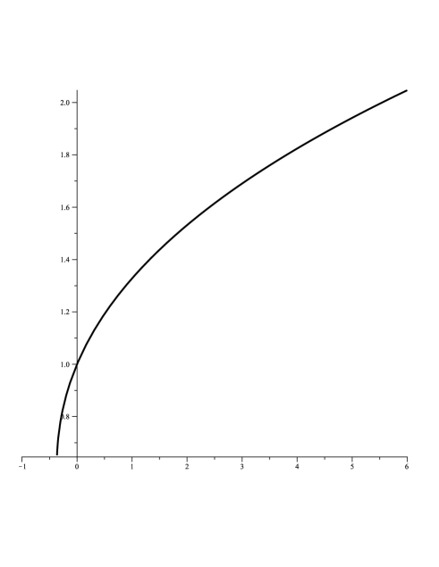
Figure 5: $e^{\frac{LambertW(x)}{2}}$ versus $x$, which shows that $e^{\frac{LambertW(x)}{2}}\geq 1$ for $x\geq 0$.

It is clear to find that $(\partial^{2}\mathcal{M}/\partial S^{2})_{Q}$ is positive for BINEF and LNEF branches. Considering ENEF branch, one may find that $e^{\frac{L_{W_{+}}}{2}}\geq 1$ and therefore $(\partial^{2}\mathcal{M}/\partial S^{2})_{Q}$ is positive (see Fig. 5 for more details). Since the temperature of the black hole solutions is positive, it is clear that the black holes are stable in the canonical ensemble.

III Asymptotic BTZ solutions

Here we would like to find that for large distance ($r>>1$), the obtained solutions are the same as charged BTZ solution. To do this, firstly, we expand Eq. (11) for the large values of $r$ which leads to

$$\left.h(r)\right|_{\text{Large }r}=q\ln\left(\frac{r}{l}\right)+\left\{\begin{array}[]{ll}\frac{q^{3}}{4r^{2}\beta^{2}}-\frac{3q^{5}}{32r^{4}\beta^{4}}+O\left(\frac{1}{r^{6}}\right),&\text{BINEF}\vspace{0.1cm}\\ \frac{q^{3}}{r^{2}\beta^{2}}-\frac{5q^{5}}{2r^{4}\beta^{4}}+O\left(\frac{1}{r^{6}}\right),&\text{ENEF}\vspace{0.1cm}\\ \frac{q^{3}}{8r^{2}\beta^{2}}-\frac{q^{5}}{32r^{4}\beta^{4}}+O\left(\frac{1}{r^{6}}\right),&\text{LNEF}\end{array}\right..$$ (39)

It is easy to find that for large $r$, the dominant (first) term of $h(r)$ for all the mentioned NLED fields is the same as one in BTZ solution BTZ1 ; BTZ2 . Differentiating from Eq. (39) or expanding Eq. (12) for large distance, one can obtain

$$F_{tr}=\frac{q}{r}+\left\{\begin{array}[]{ll}-\frac{q^{3}}{2\beta^{2}r^{3}}+\frac{3q^{5}}{8\beta^{4}r^{5}}+O\left(\frac{1}{r^{7}}\right),&\text{BINEF}\\ -\frac{2q^{3}}{\beta^{2}r^{3}}+\frac{10q^{5}}{\beta^{4}r^{5}}+O\left(\frac{1}{r^{7}}\right),&\text{ENEF}\\ -\frac{q^{3}}{4\beta^{2}r^{3}}+\frac{q^{5}}{8\beta^{4}r^{5}}+O\left(\frac{1}{r^{7}}\right),&\text{LNEF}\end{array}\right.,$$ (40)

which its dominant (first) term is similar to the electrical field of $(2+1)$-dimensional Reissner-Nordström black hole.

Now, we focus on the metric function. Straightforward calculations show that expansion of $f(r)$ in Eq. (14) for $r>>1$, leads to the following equation

$$f(r)=\frac{r^{2}}{l^{2}}-M-2q^{2}\ln\left(\frac{r}{l}\right)+\left\{\begin{array}[]{ll}-\frac{q^{4}}{4r^{2}\beta^{2}}+\frac{q^{6}}{16r^{4}\beta^{4}}+O\left(\frac{1}{r^{6}}\right),&\text{BINEF}\vspace{0.2cm}\\ -\frac{q^{4}}{r^{2}\beta^{2}}+\frac{5q^{6}}{3r^{4}\beta^{4}}+O\left(\frac{1}{r^{6}}\right),&\text{ENEF}\vspace{0.2cm}\\ -\frac{q^{4}}{8r^{2}\beta^{2}}+\frac{q^{6}}{48r^{4}\beta^{4}}+O\left(\frac{1}{r^{6}}\right),&\text{LNEF}\end{array}\right..$$ (41)

One may ignore small charge terms to find laps function of $(2+1)$-dimensional BTZ black hole.

IV Conclusions

Considering the nonlinear electromagnetic fields in various sciences is one of the interests but with cumbersome calculations. In this paper, we introduced three kinds of NLED theories which in the weak field approximation (large values of nonlinearity parameter: $\beta\longrightarrow\infty$) become the usual linear Maxwell theory. In addition, as we have shown, presented solutions have the following properties:

First, obtained electromagnetic fields have regular behavior for large values of distance and they are finite near the origin. In addition, we showed that the effect of nonlinearity parameter, on the strength of electromagnetic fields is more considerable for small values of distances. It is so interesting that $F_{tr}^{ENEF}$ diverges at $r=0$, but its divergency is very slower than the electromagnetic field of BTZ solution.

Second, all obtained solutions have a timelike curvature singularity at $r=0$, and they are asymptotic AdS. In other word, the NLED fields have no effect on the existence of singularity and asymptotic behavior, but we should note that the nonlinearity of electromagnetic field reduces the strength of singularity. Furthermore, for small values of the nonlinearity parameter, ($\beta<\beta_{c}$), the singularity covered with a non-extreme horizon. In other word, in this case the horizon geometry of nonlinear charged black holes is close to the horizon of uncharged (Schwarzschild) black hole solution.

Third, obtained solutions have different temperature and electric potential, but the same entropy and electric charge. We should note that, unlike the solutions of Einstein-power Maxwell invariant gravity PMIpaper , the electric charge is the same as Maxwell field and the nonlinearity has no effect on it.

Fourth, one may confirm that all obtained solutions reduce to the charged BTZ black hole for large values of distance.

As final remarks, we should note that the conserved and thermodynamic quantities satisfy the first law of thermodynamics and the presented solutions have positive heat capacity, which means that the black holes are stable for all the allowed values of the metric parameters.

It is worthwhile to investigate the dynamical stability of the presented solutions and also generalize these three dimensional solutions to higher dimensional case with various horizon topologies, and these problems are left for the future.

References

• (1) E. S. Fradkin and A. A. Tseytlin, Phys. Lett. B 163, 123 (1985); E. Bergshoeff, E. Sezgin, C. N. Pope and P. K. Townsend, Phys. Lett. B 188, 70 (1987); R. R. Metsaev, M. A. Rahmanov and A. A. Tseytlin, Phys. Lett. B 193, 207 (1987); A. A. Tseytlin, Nucl. Phys. B 501, 41 (1997); D. Brecher and M. J. Perry, Nucl. Phys. B 527, 121 (1998).
• (2) M. Born and L. Infeld, Proc. R. Soc. London A 143, 410 (1934); M. Born and L. Infeld, Proc. R. Soc. London A 144, 425 (1934).
• (3) R. G. Leigh, Mod. Phys. Lett. A 4, 2767 (1989).
• (4) B. Hoffmann, Phys. Rev. 47, 877 (1935).
• (5) M. H. Dehghani and H. R. Sedehi, Phys. Rev. D 74, 124018 (2006); D. L. Wiltshire, Phys. Rev. D 38, 2445 (1988); M. Aiello, R. Ferraro and G. Giribet, Phys. Rev. D 70, 104014 (2004); M. H. Dehghani and S. H. Hendi, Int. J. Mod. Phys. D 16, 1829 (2007); M. H. Dehghani, S. H. Hendi, A. Sheykhi and H. R. Rastegar-Sedehi, JCAP, 02, 020 (2007); M. H. Dehghani, N. Alinejadi and S. H. Hendi, Phys. Rev. D 77, 104025 (2008); S. H. Hendi, J. Math. Phys. 49, 082501 (2008).
• (6) M. Hassaine and C. Martinez, Phys. Rev. D 75, 027502 (2007); S. H. Hendi and H. R. Rastegar-Sedehi, Gen. Relativ. Gravit. 41, 1355 (2009); S. H. Hendi, Phys. Lett. B 677, 123 (2009); M. Hassaine and C. Martinez, Class. Quantum Gravit. 25, 195023 (2008); H. Maeda, M. Hassaine and C. Martinez, Phys. Rev. D 79, 044012 (2009); S. H. Hendi and B. Eslam Panah, Phys. Lett. B 684, 77 (2010); S. H. Hendi, Phys. Lett. B 690, 220 (2010); S. H. Hendi, Prog. Theor. Phys. 124, 493 (2010); S. H. Hendi, Eur. Phys. J. C 69, 281 (2010); S. H. Hendi, Phys. Rev. D 82, 064040 (2010).
• (7) E. Ayon-Beato and A. Garcia, Phys. Rev. Lett. 80, 5056 (1998).
• (8) H. P. de Oliveira, Class. Quantum Gravit. 11, 1469 (1994).
• (9) H. H. Soleng, Phys. Rev. D 52, 6178 (1995).
• (10) H. P. Oliveira, Class. Quantum Gravit. 11, 1469 (1994).
• (11) D. Palatnik, Phys. Lett. B 432, 287 (1998).
• (12) E. Ayon–Beato and A. Garcia, Phys. Rev. Lett. 80, 5056 (1998).
• (13) E. Ayon–Beato and A. Garcia, Gen. Relativ. Gravit. 31, 629 (1999).
• (14) E. Ayon–Beato and A. Garcia, Phys. Lett. B 464, 25 (1999).
• (15) D. A. Rasheed, [hep-th/9702087].
• (16) G. Boillat, J. Math. Phys. 11, 941 (1970); 11, 1482 (1970).
• (17) G. W. Gibbons and D. A. Rasheed, Nucl. Phys. B 454, 185 (1995).
• (18) R. Gopakumar, S. Minwalla, N. Seiberg, A. Strominger, JHEP 0008, 008 (2000).
• (19) T. Tamaki and K. Maida, Phys. Rev. D 62, 084041 (2000); H. Yajima and T. Tamaki, Phys. Rev. D 63, 064007 (2001).
• (20) S. Kar and S. Majumdar, Int. J. Mod. Phys. A 21, 6087 (2006).
• (21) M. Brigante, H. Liu, R. C. Myers, S. Shenker and S. Yaida, Phys. Rev. D 77, 126006 (2008); Y. Kats and P. Petrov, JHEP 01, 044 (2009).
• (22) P. Kovtun, D. T. Son and A. O. Starinets, JHEP 10, 064 (2003).
• (23) R-G. Cai and Y-W. Sun, JHEP 09, 115 (2008).
• (24) X-H. Ge, Y. Matsuo, F-W. Shu, S-J. Sin and T. Tsukioka, JHEP 10, 009 (2008).
• (25) J. Jing and S. Chen, Phys. Lett. B 686, 68 (2010).
• (26) R. Gregory, S. Kanno and J. Soda, JHEP 10, 010 (2009).
• (27) Q. Y. Pan, B. Wang, E. Papantonopoulos, J. Oliveira and A. Pavan, Phys. Rev. D 81, 106007 (2010).
• (28) H. J. Mosquera Cuesta and J. M. Salim, Mon. Not. Roy. Astron. Soc. 354, L55 (2004).
• (29) H. J. Mosquera Cuesta and J. M. Salim, Ap. J. 608, 925 (2004).
• (30) M. Banados, C. Teitelboim and J. Zanelli, Phys. Rev. Lett. 69, 1849 (1992).
• (31) M. Banados, M. Henneaux, C. Teitelboim and J. Zanelli, Phys. Rev. D 48, 1506 (1993).
• (32) S. Nojiri and S. D. Odintsov, Mod. Phys. Lett. A 13, 2695 (1998); R. Emparan, G. T. Horowitz and R. C. Myers, JHEP 0001, 021 (2000); S. Hemming, E. Keski-Vakkuri and P. Kraus, JHEP 0210, 006 (2002); M. R. Setare, Class. Quantum Gravit. 21, 1453 (2004); B. Sahoo and A. Sen, JHEP 0607, 008 (2006); M. R. Setare, Eur. Phys. J. C 49, 865 (2007); M. Cadoni and M. R. Setare, JHEP 0807, 131 (2008); M. Park, Phys. Rev. D 77, 026011 (2008); M. Park, Phys. Rev. D 77, 126012 (2008); J. Parsons and S. F. Ross, JHEP 0904, 134 (2009); M. R. Setare and M. Jamil, Phys. Lett. B 681, 469 (2009).
• (33) S. Carlip, Class. Quantum Gravit. 12, 2853 (1995).
• (34) A. Ashtekar, Adv. Theor. Math. Phys. 6, 507 (2002).
• (35) T. Sarkar, G. Sengupta and B. Nath Tiwari, JHEP 0611, 015 (2006);
• (36) E. Witten, Adv. Theor. Math. Phys. 2, 505 (1998).
• (37) S. Carlip, Class. Quantum Gravit. 22, R85 (2005).
• (38) E. Witten, [arXiv:07063359].
• (39) S. P. Kim, S. K. Kim, K. S. Soh and J. H. Yee, Phys. Rev. D 55, 2159 (1997); G. W. Gibbons, M. J. Perry and C. N. Pope, Class. Quantum Gravit. 22, 1503 (2005); J. E. Aman and N. Pidokrajt, Phys. Rev. D 73, 024017 (2006).
• (40) H. Saida and J. Soda, Phys. Lett. B 471, 358 (2000).
• (41) M. Cadoni, M. Melis and M. R. Setare, Class. Quantum Gravit. 25, 195022 (2008).
• (42) A. Larranaga, [arXiv:10023416].
• (43) S. Hyun, J. Korean Phys. Soc. 33, S532 (1998).
• (44) K. Sfetsos and K. Skenderis, Nucl. Phys. B 517, 179 (1998).
• (45) F. Canfora and A. Giacomini, [arXiv:10050091].
• (46) L. Claessens, [arXiv:09122245]; L. Claessens, [arXiv:09122267].
• (47) S. H. Hendi, Eur. Phys. J. C 71, 1551 (2011).
• (48) J. T. Liu and P. Szepietowski, Phys. Rev. D 79, 084042 (2009); Y. Kats, L. Motl and M. Padi, JHEP 0712, 068 (2007); D. Anninos and G. Pastras, JHEP 0907, 030 (2009); R. G. Cai, Z. Y. Nie and Y. W. Sun, Phys. Rev. D 78, 126007 (2008).
• (49) D. J. Gross and J. H. Sloan, Nucl. Phys. B 291, 41 (1987).
• (50) E. A. Bergshoeff and M. de Roo, Nucl. Phys. B 328, 439 (1989).
• (51) W. A. Chemissany, M. de Roo and S. Panda, JHEP 0708, 037 (2007).
• (52) M. Natsuume, Phys. Rev. D 50, 3949 (1994).
• (53) D. Garfinkle, G. T. Horowitz and A. Strominger, Phys. Rev. D 43, 3140 (1991) [Erratum ibid. 45, 3888 (1992)].
• (54) A. Ritz and R. Delbourgo, Int. J. Mod. Phys. A 11, 253 (1996).
• (55) W. Heisenberg and H. Euler, Z. Phys. 98, 714 (1936); Translation by W. Korolevski and H. Kleinert, [physics/0605038]
• (56) B. L. Altshuler, Class. Quantum Gravit. 7, 189 (1990).
• (57) R. C. Myers, Phys. Rev. D 36, 392 (1987); S. C. Davis, Phys. Rev. D 67, 024030 (2003).
• (58) M. Cataldo and A. Garcia, [arXiv:hep-th/9903257]; R. Yamazaki and D. Ida, [arXiv:gr-qc/0105092]; Y. S. Myung, Y. W. Kim, and Y. J. Park, [arXiv:0804.0301].
• (59) R. M. Corless, G. H. Gonnet, D. E. G. Hare, D. J. Jeffrey and D. E. Knuth, Adv. Computational Math. 5, 329 (1996).
• (60) M. Cvetic and S. S. Gubser, JHEP. 04, 024 (1999); M. M. Caldarelli, G. Cognola and D. Klemm, Class. Quantum Gravit. 17, 399 (2000).
• (61) J. D. Bekenstein, Lett. Nuovo Cimento 4, 737 (1972); J. D. Bekenstein, Phys. Rev. D 7, 2333 (1973); S. W. Hawking and C. J. Hunter, Phys. Rev. D 59, 044025 (1999).
• (62) S. W. Hawking, C. J. Hunter and D. N. Page, Phys. Rev. D 59, 044033 (1999); R. B. Mann, Phys. Rev. D 60, 104047 (1999); R. B. Mann, Phys. Rev. D 61, 084013 (2000); C. J. Hunter, Phys. Rev. D 59, 024009 (1999).