The HIFI spectral survey of AFGL 2591 (CHESS).
II. Summary of the survey.

Abstract

Aims. This paper presents the richness of submillimeter spectral features in the high-mass star forming region AFGL 2591.

Methods. As part of the CHESS (Chemical Herschel Survey of Star Forming Regions) Key Programme, AFGL 2591 was observed by the Herschel/HIFI instrument. The spectral survey covered a frequency range from 480 up to 1240 GHz as well as single lines from 1267 to 1901 GHz (i.e. CO, HCl, NH₃, OH and [CII]). Rotational and population diagram methods were used to calculate column densities, excitation temperatures and the emission extents of the observed molecules associated with AFGL 2591. The analysis was supplemented with several lines from ground-based JCMT spectra.

Results. From the HIFI spectral survey analysis a total of 32 species were identified (including isotopologues). In spite of the fact that lines are mostly quite weak ($\rm{\int{T_{mb}dV}}$$\sim$ few $\rm{K\,km\,s^{-1}}$), 268 emission and 16 absorption lines were found (excluding blends). Molecular column densities range from 6 $\times\,10^{11}$ to 1 $\times\,10^{19}$ cm^-2 and excitation temperatures range from 19 to 175 K. One can distinguish cold (e.g. HCN, H₂S, NH₃ with temperatures below 70 K) and warm species (e.g. CH₃OH, SO₂) in the protostellar envelope.

1 Introduction

Massive stars play a major role in the evolution of galaxies. From their birth in dense molecular clouds to their death as a supernova explosion, massive stars interact heavily with their surroundings by emitting strong stellar winds and by creating heavy elements (Zinnecker & Yorke 2007). They influence the formation of nearby low-mass stars and planets (Bally et al. 2005) as well the physical, chemical and morphological structure of galaxies (e.g., Kennicutt & Evans 2012). Although, massive stars are an important component of galaxies, their formation processes are still unclear. It is difficult to observe high-mass star forming regions because of high dust extinction, their large distances and rapid evolution (Tan et al. 2014).

High-mass star forming regions are quite rare, so each observational effort is very helpful in solving their puzzle. One of the goals of the Herschel Space Observatory (Pilbratt et al. 2010) was to improve our understanding of the high-mass star formation processes. Among the several Key Projects devoted to those studies, we focus here on the Herschel Key Program CHESS (Chemical Herschel Survey of Star Forming Regions, Ceccarelli & CHESS Consortium 2010). The aim of this project is to study the chemical composition of dense regions of the interstellar medium, to understand the chemical evolution of star forming regions and the differences between regions with different masses/luminosities. The target sources of CHESS are the pre-stellar cores I16293E and L1544, the outflow shock spot L1157-B1, the low-mass protostar IRAS16293-2422, the intermediate-mass protostar OMC2-FIR 4, the intermediate luminosity hot cores NGC 6334I and AFGL 2591 and the high luminosity hot core W51e1/e2. Almost the entire spectral range of the HIFI instrument, i.e. 480 to 1910 $\rm{GHz}$, has been used for the observation of the above listed objects. In this paper we will focus on the source AFGL 2591.

Spectral surveys cover simultaneously a large variety of molecular and atomic lines. In this way they offer the possibility to probe cold and warm gas and the fundamental processes which occur in star forming regions. Especially, Herschel’s large frequency range allowed to cover molecular lines from very different energy levels, from light to heavier molecules and therefore study species thoroughly.

AFGL 2591 is one of the CHESS sources. It is a relatively isolated high-mass protostellar object with a bipolar molecular outflow (Van der Tak et al. 1999). A massive sub-Keplerian disk has been proposed to exist around source AFGL 2591–VLA 3 (Wang et al. 2012). AFGL 2591 is located in the Cygnus X region, (l, b) = 78.$\degr$9, 0.$\degr$71. Based on VLBI parallax measurements of 22 GHz water maser, Rygl et al. (2012) have estimated recently the distance towards AFGL 2591 of 3.33 $\pm$ 0.11 kpc, hence, the corresponding luminosity is L = 2 $\times\,10^{5}$ L_☉ (Sanna et al. 2012). For a detailed source description see Van der Wiel et al. (2013) (hereafter Paper I) and references therein.

The richness of the detected lines in AFGL 2591 from the HIFI/CHESS spectral survey gives us the opportunity to gain detailed insights into its chemical and physical structure. Results from the spectral survey are going to be presented in a series of papers. The first one focused on highly excited linear rotor molecules (Van der Wiel et al. 2013). In the present work the entire HIFI spectral survey of AFGL 2591 is presented.

Van der Wiel et al. (2013) studied linear rotor molecules (CO, HCO${}^{+},$ CS, HCN, HNC) in the high-mass protostellar envelope. This work was based on the Herschel/HIFI data together with observations from the ground-based telescopes, JCMT and IRAM 30m. The line profiles of the observed emissions consist of two components, a narrow one which corresponds to the envelope and a broad component from the outflow. The same nomenclature is used in the present paper.

This paper starts with the description of the observations and the data reduction of Herschel and JCMT spectra (Sect. 2). In Sect. 3 the general summary of the HIFI/CHESS spectral survey of AFGL 2591 is given. Here, all of the observed species from that survey are presented together with emission and absorption lines analysis. Discussions and conclusions are given in Sects. 5 and 6, respectively. Appendix A gives a table with all detected transitions and plots of their line profiles.

2 Observations and data reduction

2.1 480–1850 GHz Herschel/HIFI data

Observations of AFGL 2591 ($\alpha_{2000}$ $=$ 20^h29^m24^s.9, $\delta_{2000}$ $=$ +40${\degr}$11$\arcmin$21$\arcsec$) were obtained with the Heterodyne Instrument for the Far-Infrared (HIFI, de Graauw et al. 2010) onboard the ESA Herschel Space Observatory as a part of the HIFI/CHESS Guaranteed Time Key Programme.

A full spectral survey of AFGL 2591 of HIFI bands 1a – 5a (480 – 1240 $\rm{GHz}$, 18.4 h of observing time) was obtained. Nine additional selected frequencies were observed in 3.5 h of observing time. The corresponding bands are: 5b (lines: HCl, CO), 6a (CO), 6b (CO), 7a (NH₃, CO) and 7b (CO, OH, [CII]).

Despite being the second in a series of papers based on HIFI/CHESS data of AFGL 2591 and detailed description of its data reduction process in Paper I (Van der Wiel et al. 2013), basic information is recalled here as well.

The spectral scan observations were carried out using the dual beam switch (DBS) mode, with the Wide Band Spectrometer (WBS) with a resolution of 1.1 MHz, corresponding to 0.66 $\rm{km\,s^{-1}}$ at 500 GHz and 0.18 $\rm{km\,s^{-1}}$ at 1850 GHz. The single frequency settings were obtained in the dual beam switch mode as well, with the fast chop and stability optimization options selected. Table 1 gives information about the covered frequency range, beam size, noise level, and integration time.

Table 1: Overview over all HIFI bands for the observations of AFGL 2591 (bands: 1a – 5a are spectral scans, 5b – 7b single frequency settings).

Band	Freq. range	Beam size	rms	Obs. time
	[GHz]	[”]	[K]	[s]
1a	483–558	41	0.030	4591
1b	555–636	36	0.029	4643
2a	631–722	31	0.026	9833
2b	717–800	28	0.067	6407
3a	800–859	26	0.039	4893
3b	858–960	23	0.067	8578
4a	950–1060	21	0.157	9137
4b	1051–1120	20	0.144	6300
5a	1110–1240	18	0.147	11931
5b	1266–1270	17	0.149	1380
5b	1251–1255	17	0.149	2255
6a	1496–1499	14	0.117	1440
6b	1611–1614	13	0.106	1392
7a	1726–1729	12	0.092	1575
7a	1762–1764	12	0.095	1423
7b	1840–1843	12	0.092	1711
7b	1900–1903	12	0.120	1452

AFGL 2591 data were completely reduced with the HIPE–Herschel Interactive Processing Environment (Ott 2010), version 8.1, using scripts written by the CHESS data reduction team (Kama et al. 2013). After pipelining, the quality of each spectrum was checked and spectral regions with spurious features (spurs) were flagged. Next, the correction for standing waves was made and a baseline was subtracted (polynomial of order $\sim$3). The final single sideband spectrum is presented in Fig. 1.

Figure 1: Complete baseline-subtracted spectrum. The strongest lines belong to CO and its isotopologues, while at 1901 GHz [CII] is seen.

Strong lines are known to create ghost features in the sideband deconvolution process (Comito & Schilke 2002). To check the importance of this effect on our data, the above steps were repeated with strong lines (especially CO transitions) masked out in the same way as spurs. The term strong lines refers to features of $T_{A}^{*}>$1 K in band 1a to $>$8 K in band 5a, depending on the amount of lines and the noise level in a given band. Following the outlined data reduction procedure, two single sideband spectra for bands 1a – 5a were obtained. The first set of spectra was used to analyse strong lines (e.g. CO and its isotopologues, HCO⁺). The second one, for line measurements of weak features, i.e. which were not masked as strong lines (e.g. SO, CH₃OH).

2.2 330–373 GHz JCMT data

The excitation analysis of several molecules was complemented by ground-based observations from the James Clerk Maxwell Telescope (JCMT). These data are part of the JCMT Spectral Legacy Survey (SLS, Plume et al. 2007). The observations were taken with the 16-element Heterodyne Array Receiver Programme B (HARP-B) and the Auto-Correlation Spectral Imaging System (ACSIS) correlator (Dent et al. 2000; Smith et al. 2008; Buckle et al. 2009).

The JCMT survey of AFGL 2591 covers the frequency range of 330 – 373 $\rm{GHz}$ with a spectral resolution of 1 MHz ($\sim$ 0.8  $\rm{km\,s^{-1}}$). The beam size of the JCMT at these frequencies is 14 – 15^′′, the image size is 2^′. Detailed information about the data reduction and analysis can be found in (Van der Wiel et al. 2011).

3 The HIFI spectral survey of AFGL 2591

3.1 Detections and line profiles

Figure 2: The average values of the line widths (top panel) and the average values of the central velocity (bottom panel) from Gaussian fits for the observed emission lines of different molecules (”o” represents the outflow component). The emission lines of the envelope component are centered at $-5.5$ $\rm{km\,s^{-1}}$, as shown by a dashed line at the bottom panel.

From the Herschel/HIFI spectral survey, a total of 32 species (including isotopologues) were identified, resulting in 252 emission and 16 absorption lines (218 different transitions). Blended features were excluded from the analysis. Herschel surveys toward different sources revealed many spectral features which are not possible to be identified at this moment (e.g. Wang et al. 2011). However, no unidentified lines were found in our spectra.

For the line identification the JPL (Pickett et al. 1998) and CDMS (Müller et al. 2001, 2005) databases were used. Line analysis was made with the CASSIS software. The presence of possible transitions resulting from an upper energy level E_up of less than 500 K was checked. Generally, detected lines have E_up$<$ 400 K, except for the high–J CO transitions, which have E_up up to 752 K.

All the detected lines in the HIFI survey are presented in Table LABEL:table:measurement, the entire spectrum is shown in Fig. 1 and corresponding line profiles can be found in Figures 5. For the sake of completeness all of the observed lines together with their profiles and measurements are presented in Table LABEL:table:measurement, including the datasets of Paper I (Van der Wiel et al. 2013) and the complementary JCMT data.

Although the analysis of our survey revealed no new molecular species, some of our observed species have not been seen toward AFGL 2591 before. HIFI with its broad spectral range gave the opportunity to observe for the first time in AFGL 2591 transitions of: HF (Emprechtinger et al. 2012), OH⁺, CH, CH⁺ (Bruderer et al. 2010b) or C⁺ and HCl (this work).

Within the object AFGL 2591, CH₃OH, SO₂ and SO show the highest number of detected transitions (54, 26 and 18 lines, respectively) among its identified species, followed by H₂CO as well as CO and its isotopologues. In the cases of the other molecules, at most a few lines were observed. The strongest transitions originate from CO and its isotopologues, HCO⁺, H₂O and OH. In comparison, the remaining detected lines are relatively weak due to fluxes below 1 $\rm{K\,km\,s^{-1}}$.

The line measurements were done in the same way as described in Paper I. A Gaussian profile was fitted to each line, using the Levenberg-Marquardt fitter in the line analysis module of CASSIS. For most lines, a single Gaussian profile gave a good fit to the profile. However, in cases of CO, ¹³CO, C¹⁸O, CI, [CII], HCO⁺, OH and H₂O double Gaussian profiles were needed to fit sufficiently narrow and broad line components. The measured parameters from Gaussian fits of the emission lines (central velocity and full width at half maximum) are plotted in Fig. 2 (together with the complementary JCMT data) as an average value for each molecule.

The narrow and single line components are centered at $-$5.5 $\pm$ 0.5 $\rm{km\,s^{-1}}$, (as derived before by Van der Tak et al. 1999) and originate from the protostellar envelope. Their line widths are of the order of 3.7 $\pm$ 0.9 $\rm{km\,s^{-1}}$. Whereas, the broader line components (10.9 $\pm$ 4.2 $\rm{km\,s^{-1}}$) are caused by the outflows and are centered at $-$6.3 $\pm$ 0.7 $\rm{km\,s^{-1}}$. It was shown in Paper I that the outflow gas is not significantly different from that in the envelope, considering gas density, gas temperature, as well as the chemical balance of CO and HCO⁺.

3.2 Absorption line analysis

Table 2: Fit results for absorptions.

Molecule	$\rm{V_{lsr}}$a	$\Delta$Va	N
	[$\rm{km\,s^{-1}}$]	[$\rm{km\,s^{-1}}$]	[cm-2]
CCH	0.82	2.58	3.3$\pm$1.0 $\times$ 1017
CHb	0.21	2.19	3.1$\pm$0.9 $\times$ 1013
CH+	4.17	12.42	1.1$\pm$0.4 $\times$ 1014
H2S	0.22	0.97	3.5$\pm$0.9 $\times$ 1012
NH3	0.00	1.30	1.8$\pm$0.8 $\times$ 1012
H2Ob	-0.50	2.43	1.5$\pm$0.6 $\times$ 1013
OH+b	3.65	9.13	3.0$\pm$1.0 $\times$ 1013
HF	-0.05	2.31	5.2$\pm$1.3 $\times$ 1012
HF	-3.88	2.50	5.5$\pm$1.4 $\times$ 1012
H2O	-11.98	13.75	2.3$\pm$0.6 $\times$ 1013
CH+	-16.90	9.24	6.8$\pm$1.3 $\times$ 1013
HF	-12.58	8.81	1.8$\pm$0.6 $\times$ 1013

• Errors of $\rm{V_{lsr}}$and $\Delta$V are listed in Table LABEL:table:measurement.

• The average of a few lines from the same velocity component: 2 lines of CH, 2 lines of H₂O and 3 lines of OH⁺.

There are only a few absorption features observed toward AFGL 2591. A foreground cloud at V${}_{\mbox{\scriptsize lsr}}$ $\sim$ 0 $\rm{km\,s^{-1}}$ has been detected before by e.g. Bruderer et al. (2010b); Emprechtinger et al. (2012); Van der Wiel et al. (2013). In the CHESS/HIFI dataset we found 16 absorption lines; all measurements are listed together with emissions in Table LABEL:table:measurement and their lines profiles are presented in Figures 5. Mostly they are red-shifted and associated with the foreground cloud at V${}_{\mbox{\scriptsize lsr}}$ $\sim$ 0 $\rm{km\,s^{-1}}$. Three broad, blue-shifted absorptions belong to the outflow lobe.

We derived the molecular column densities using the following relations:

$$\rm{N_{tot}}=\rm{N_{l}}\frac{\rm{Q(T_{ex})}}{\rm{g_{l}}}exp\left({\frac{E_{l}}{kT_{ex}}}\right)\ [cm^{-2}]$$ (1)

$$\rm{N_{l}}=\frac{8\pi\nu^{3}}{c^{3}}\frac{\rm{g_{l}}}{\rm{g_{u}}\rm{A_{ul}}}\int\tau\cdot dv\ [cm^{-2}]$$ (2)

where $\rm{Q(T_{ex})}$ is the partition function computed at the excitation temperature $\rm{T_{ex}}$, $\nu$ is the frequency of the observed transition with the Einstein A-coefficient $\rm{A_{ul}}$ and the statistical weights of the lower $\rm{g_{l}}$ and upper levels $\rm{g_{u}}$; c is the speed of light and k is the Boltzmann constant. The line opacity $\tau$ was calculated from the measured brightness temperature $\rm{T_{mb}}$ and the temperature of the background continuum in a single side band $\rm{T_{c}}$, using the relation  $\tau=-ln(\frac{\rm{T_{mb}}}{\rm{T_{c}}})$.

$\rm{N_{tot}}$ and $\rm{N_{l}}$ are the total column density and the column density in the lower state of transition, respectively. The $\rm{N_{l}}$ may be the same as total column density for the ground state lines, when the excitation temperature is very low ($\rm{T_{ex}}$ $\sim$ 2.73 K). Thus for the ground state transitions we applied the Eq. 2 to calculate column densities. For the absorptions that arise from the excited states we used the Eq. 1 and assumed the excitation temperature of 10 K as it was derived for the foreground cloud in Paper I (see Table 4. Van der Wiel et al. 2013).

The tentative absorption lines from a foreground cloud at V${}_{\mbox{\scriptsize lsr}}$ $\sim$ 0 $\rm{km\,s^{-1}}$ were observed of CCH (7₇-6₆ at 611.265 GHz), CH (2 transitions: $3/2_{2+}-1/2_{1-}$ at 532.724 and $3/2_{2-}-1/2_{1+}$ at 536.761 GHz), CH⁺ ($1-0$ at 835.138 GHz), H₂S ($2_{12}-1_{01}$ at 736.034 GHz), NH₃ ($1_{0}-0_{0}$ at 572.498 GHz), H₂O (2 transitions: $1_{10}-1_{01}$ at 556.936 and $1_{11}-0_{00}$ at 1113.343 GHz), OH⁺ (3 transitions: $J$=$2$–$1,F$=$3/2$–$1/2$ at 971.805, $J$=$1$–$1,F$=$3/2$–$1/2$ at 1033.004 and $J$=$1$–$1,F$=$3/2$–$3/2$ at 1033.119 GHz) and HF ($1-0$ at 1232.476 GHz). The estimated column densities for above species are listed in the upper part of Table 2.

Three broad absorptions are associated with the outflow (centered at $\sim-$ 13.8 $\rm{km\,s^{-1}}$): H₂O, CH⁺ and HF. Their column densities are presented in the lower part of Table 2.

Bruderer et al. (2010b), using HIFI, analysed hydrides toward AFGL 2591. Our column density results are in good agreement, within the errors, with their measurements: 3.1 $\times$ 10¹³ and 2.6 $\times$ 10¹³ cm^-2 for CH, 6.8 $\times$ 10¹³ and 1.8 $\times$ 10¹⁴ cm^-2 for CH⁺ outflow component, 1.1 $\times$ 10¹⁴ and 1.2 $\times$ 10¹⁴ cm^-2 for CH⁺, and 3.0 $\times$ 10¹³ and 6.1 $\times$ 10¹³ cm^-2 for OH⁺, our results and from (Bruderer et al. 2010b) respectively. Bruderer et al. (2010b) in their spectra found also lines of NH and H₂O⁺. These two species are not seen in our dataset, because of a slightly lower quality of spectral scans (Bruderer et al. (2010b) have observations from the single frequency settings).

Recently, based on Herschel data, (Barlow et al. 2013) detected in the Crab Nebula emission lines of  ³⁶ArH⁺. Absorptions of this ion are also seen toward sources from HEXOS (Herschel Observations of EXtra-Ordinary Sources) and PRISMAS (PRobing InterStellar Molecules with Absorption line Studies) Herschel Key Programs (Schilke et al. 2014). The ³⁶ArH⁺ J=1-0 transition at 617.525 GHz is not seen in our spectra. The upper limit of a column density is 7.7 $\times$ 10¹² cm^-2 for the width of an absorption line of 1 $\rm{km\,s^{-1}}$.

3.3 Emission line analysis

Table 3: Parameters estimated from rotational and population diagrams methods (column densities, excitation temperatures and emission extents) based on HIFI and JCMT data.

Molecule	V	FWHM	Rotational		Population			$\tau$	Eup range	No of trans.
	[$\rm{km\,s^{-1}}$]	[$\rm{km\,s^{-1}}$]	N${}_{\mbox{\scriptsize col}}$[cm-2]	T${}_{\mbox{\scriptsize ex}}$[K]	N${}_{\mbox{\scriptsize col}}$[cm-2]	T${}_{\mbox{\scriptsize ex}}$[K]	size[′′]		[K]
CO	-4.8±0.3	5.1±0.9	6.0 $\times$ 1016 ${}_{-0.5}^{+0.5}$	162${}_{-9}^{+10}$	1.2 $\times$ 1019 ${}_{-0.6}^{+0.4}$	62${}_{-6}^{+4}$	17${}_{-7}^{+3}$	0.1–144	33–752	12
	-7.2±2.3	15.4±1.8	6.0 $\times$ 1016 ${}_{-1.0}^{+1.0}$	89${}_{-9}^{+10}$	8.0 $\times$ 1018 ${}_{-0.4}^{+0.4}$	42${}_{-2}^{+2}$	17${}_{-1}^{+1}$	0.01–34	33–752	12
HCO+	-5.6±0.2	3.4±0.4	2.3 $\times$ 1013 ${}_{-1.0}^{+1.0}$	35${}_{-3}^{+3}$	1.0 $\times$ 1014 ${}_{-1.0}^{+1.0}$	43${}_{-3}^{+2}$	11${}_{-1}^{+1}$	0.08–2.02	43–283	7
	-6.8±0.6	7.3±2.0	2.2 $\times$ 1013 ${}_{-1.6}^{+4.2}$	23${}_{-15}^{+15}$	2.0 $\times$ 1015 ${}_{-1.6}^{+3.3}$	19${}_{-2}^{+9}$	9.7${}_{-2.4}^{+0.8}$	0.7–35	43–154	4
HCN	-5.3±0.2	4.2±0.7	4.5 $\times$ 1013 ${}_{-0.5}^{+0.7}$	31${}_{-10}^{+14}$	1.1 $\times$ 1015 ${}_{-0.7}^{+0.8}$	35${}_{-1}^{+1}$	7.7${}_{-0.2}^{+0.2}$	0.2–4.4	43–234	6
HNC	-5.4±0.1	3.8±0.5	4.8 $\times$ 1012 ${}_{-0.5}^{+6.3}$	43${}_{-7}^{+9}$					44–122	3
CCH	-6.3±0.5	3.7±0.5	2.2 $\times$ 1014 ${}_{-0.2}^{+0.3}$	22${}_{-3}^{+3}$	1.1 $\times$ 1016 ${}_{-0.5}^{+1.1}$	25${}_{-5}^{+6}$	5.3${}_{-0.6}^{+0.8}$	0.3–7.1	42–151	4
CN	-5.6±0.2	3.2±0.5	9.7 $\times$ 1013 ${}_{-0.7}^{+0.8}$	22${}_{-1}^{+1}$	1.3 $\times$ 1014 ${}_{-0.3}^{+0.3}$	26${}_{-3}^{+4}$	23${}_{-4}^{+6}$	0.01–0.18	33–114	3
CS	-5.5±0.4	3.9±0.5	7.4 $\times$ 1013 ${}_{-0.4}^{+0.5}$	26${}_{-10}^{+12}$	4.9 $\times$ 1013 ${}_{-0.6}^{+14.6}$	61${}_{-19}^{+7}$	14${}_{-9}^{+4}$	0.01–0.09	66–282	7
H2S	-5.7±0.7	3.4±0.8	1.1 $\times$ 1013 ${}_{-0.7}^{+1.1}$	56${}_{-14}^{+25}$	4.9 $\times$ 1014 ${}_{-0.6}^{+0.9}$	26${}_{-2}^{+3}$	8.9${}_{-0.7}^{+0.6}$	0.01–5.6	55–350	5
NH3	-5.1±0.6	4.1±1.0	2.8 $\times$ 1013 ${}_{-0.2}^{+0.3}$	67${}_{-5}^{+6}$	4.8 $\times$ 1013 ${}_{-2.4}^{+11}$	28${}_{-6}^{+3}$	9.6${}_{-0.6}^{+1.8}$	0.1–1.6	28–170	5
N2H+	-5.9±0.2	2.8±0.3	5.6 $\times$ 1011 ${}_{-1.6}^{+0.1}$	19${}_{-3}^{+13}$					45–125	3
NO	-4.8±0.5	5.8±2.8	7.2 $\times$ 1015 ${}_{-0.5}^{+0.7}$	25${}_{-10}^{+14}$	1.7$\times$ 1016 ${}_{-0.5}^{+3.6}$	54${}_{-14}^{+9}$	12${}_{-6}^{+15}$	0.015–0.021	36–115	2
CH3OH	-5.7±0.5	3.3±0.6	1.8 $\times$ 1014 ${}_{-0.7}^{+1.0}$	209${}_{-62}^{+171}$	1.5 $\times$ 1017 ${}_{-0.3}^{+0.4}$	108${}_{-7}^{+10}$	1.5${}_{-0.1}^{+0.1}$	0.6–10.4	25–352	49
H2CO	-5.4±0.3	3.6±0.7	2.0 $\times$ 1013 ${}_{-0.9}^{+1.0}$	34${}_{-6}^{+12}$	9.9 $\times$ 1013 ${}_{-0.1}^{+0.1}$	41${}_{-2}^{+2}$	7.3${}_{-0.1}^{+0.1}$	0.02–0.61	32–263	14
SO	-5.5±0.4	4.9±0.7	1.5 $\times$ 1014 ${}_{-0.2}^{+0.2}$	53${}_{-20}^{+23}$	1.9 $\times$ 1016 ${}_{-0.3}^{+0.4}$	64${}_{-4}^{+2}$	2.7${}_{-0.2}^{+0.3}$	0.1–6.1	26–405	22
SO2	-5.1±0.4	4.6±0.9	3.0 $\times$ 1014 ${}_{-1.7}^{+2.0}$	92${}_{-43}^{+77}$	5.4 $\times$ 1017 ${}_{-0.6}^{+0.7}$	175${}_{-4}^{+5}$	0.9${}_{-0.1}^{+0.1}$	0.5–8.9	31-354	47
H2O	-4.8±0.9	3.1±0.6	3.5 $\times$ 1013 ${}_{-1.4}^{+3.0}$	63${}_{-15}^{+17}$	2.4 $\times$ 1015 ${}_{-0.5}^{+0.3}$	38${}_{-1}^{+1}$	9.1${}_{-0.6}^{+0.5}$	0.4–104	53–305	8
	-6.0±0.2	12.1±2.3	5.5 $\times$ 1013 ${}_{-1.9}^{+3.1}$	43${}_{-20}^{+35}$	1.0 $\times$ 1016 ${}_{-0.4}^{+0.4}$	31${}_{-3}^{+3}$	4.9${}_{-0.4}^{+0.3}$	0.2–5.7	101–305	6

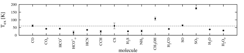
Figure 3: Column densities and excitation temperatures estimated from the population diagrams, without the uncertain measurements, ”o” sign represents the outflow component.

Figure 4: Population diagrams. Open circles represent the observational data and crosses are the best-fit model from population diagram analysis. Dotted lines correspond to a linear fit to the rotational diagram.

To estimate column densities and excitation temperatures from the observed emissions we constructed rotational diagrams which assume that all lines for a given molecule have the same excitation temperature. The rotational diagram method is a useful tool for the estimation of the column densities and the excitation temperatures when many transitions of particular species are observed. However, in many cases its accuracy is limited since it is based on the assumptions that the emission lines are optically thin and the emissions fill the beam.

Goldsmith & Langer (1999) improved this excitation analysis method by introducing correction factors for the effects of the beam dilution and optical depth. Using this population diagram method we estimated the column density, the excitation temperature and the emission extent for each molecule with the observed multiple transitions. Having three free parameters (column density, excitation temperature and the beam filling factor) we used this method only when at least 4 lines for a given molecule were observed. Otherwise, only the rotational method was applied. The rotation diagram gives beam-averaged column densities, while the population diagram gives source-averaged values. Hereafter, all stated column densities (N${}_{\mbox{\scriptsize col}}$) or excitation temperatures (T${}_{\mbox{\scriptsize ex}}$) were derived from the population diagrams, except those of HNC and N₂H⁺ which were estimated from the rotational diagrams. At this point, the complementary JCMT data were crucial to increase the number of observed transitions for a given molecule.

The column densities of CO, HCN and HCO⁺ were obtained from their isotopologues (¹³CO, C¹⁸O, C¹⁷O, H¹³CN, HC¹⁵N, H¹³CO⁺) using the standard isotopic ratios: ¹²C/¹³C = 60, ¹⁶O/¹⁸O = 500, ¹⁶O/¹⁷O = 2500 and ¹⁴N/¹⁵N = 270 (Wilson & Rood 1994).

All column densities and excitation temperatures values based on the rotational and population diagrams methods are given in Table 3. The opacities and emission sizes for each molecule derived from the population diagrams are listed in Table 3 as well. Table 3 contains also information about the covered energy E_up range for a given species and the number of lines from different energy levels which were used for the analysis. The values of the excitation temperatures and column densities are plotted in Fig. 3, excluding the uncertain measurements (i.e. HNC, N₂H⁺, CN and NO).

Based on the optical depths values from Table 3, lines of CN, CS, NO and H₂CO can be characterised as optically thin ($\tau<$ 0.6). However, results of CN and NO are uncertain because of only a few observed lines. For optically thin lines calculations based on the rotational diagrams resulted in good approximations of the column densities and the excitation temperatures. The other molecular lines were characterised as optically thick. For those molecular species the population diagram method was more accurate.

The emission extent of analysed molecules associated with AFGL 2591 ranges from around 2^′′ (species like SO, SO₂ and CH₃OH) up to 23^′′ (CN). For most species emission sizes are smaller than 17^′′.

From the comparison of the temperatures derived from the population diagrams (see the bottom panel of Fig. 3) it is possible to distinguish warm (e.g. CH₃OH, SO₂) and cold (e.g. HCN, H₂S, NH₃) species. As cold species we classify these having excitation temperatures up to 70 K. Warm molecules have higher temperatures, up to 175 K for SO₂. It is difficult to give an accurate borderline here and classify all species, however, the large range of excitation temperatures seems significant. Moreover, it was shown before by Bisschop et al. (2007) that some of the complex organic species can be classified as both, warm and cold, which may indicate that they are present in multiple physical components.

The population diagrams are presented in Fig. 4. They show evidence for excitation gradient of several species (HCO⁺, HCN, CS, SO), which means that the population diagram method may be not enough to analyse all observed molecules. This is a motivation to use in the near future more sophisticated method (i.e., radiative transfer modeling) to study our spectral survey.

4 Discussion

4.1 CI and CII

C and C⁺ are the only atomic species found in our HIFI spectral survey of AFGL 2591. Both fine-structure transitions of neutral carbon, ³P${}_{1}-^{3}$P₀ at 492 GHz and ³P${}_{2}-^{3}$P₁ at 809 GHz, were observed towards AFGL 2591. These transitions consist of two components originating from the envelope and the outflow, similar to the CO lines (see Fig. 5). CI was observed previously in AFGL 2591 by Van der Tak et al. (1999), but [CII] was observed for the first time with Herschel. The [CII] ²P${}_{3/2}-^{2}$P_1/2 line, an important interstellar coolant, shows several velocity components, two of them correspond to the ones in CI and CO. The [CII] line profile is distorted by a contamination from the off-position even after applying corrections within HIPE (Fig. 5).

4.2 CO and its isotopologues

CO is one of the most studied molecules (e.g. Mitchell et al. 1989; Black et al. 1990; Hasegawa & Mitchell 1995). Based on CO observation, Lada et al. (1984) found an extended bipolar outflow associated with AFGL 2591. Many strong lines of CO and its isotopologues (¹³CO, C¹⁸O, C¹⁷O) were also detected in our HIFI spectra showing clearly the envelope and outflow components. C¹⁷O lines are weaker, and show only the envelope components. The abundance of CO = 3 $\times$ 10^-5 was calculated in Paper I. The CO column density in this work was estimated at 1.2 $\times$ 10¹⁹ cm^-2, Van der Tak et al. (2000b) derived a similar value of 3.4 $\times$ 10¹⁹ cm^-2.

4.3 HCO⁺

HCO⁺ was identified by intense lines in the HIFI and JCMT spectra. Moreover, three lines of H¹³CO⁺ were also positively detected. The abundance of HCO⁺ was estimated at 9 $\times$ 10^-9 (Paper I) and column density at 1.0 $\times$ 10¹⁴ cm^-2. Carr et al. (1995) estimated the abundance of 4 $\times$ 10^-10 and Van der Tak et al. (1999) using a model with lower $H_{2}$ column density derived [HCO⁺] = 1 $\times$ 10^-8.

4.4 N-bearing species

Six N-bearing species were observed in the HIFI spectra: HCN, HNC, CN, NO, N₂H⁺ and NH₃. All of these molecules have been seen before in AFGL 2591 (e.g. Takano et al. 1986; Carr et al. 1995; Boonman et al. 2001). Lines of N-bearing species observed with the Herschel/HIFI are weak in comparison to CO and were sufficiently fitted with a single Gaussian profile revealing these species to be components of the protostellar envelope, centered at $-$5.5 $\rm{km\,s^{-1}}$. Only o-NH₃ shows a tentative absorption feature from a foreground cloud at V${}_{\mbox{\scriptsize lsr}}$ = 0 $\rm{km\,s^{-1}}$. Two features observed with the JCMT, HCN 4-3 and HNC 4-3 show a contribution from the outflow and double Gaussian profiles were fitted to these lines. We did not find NH and NH₂, which were seen in other HIFI spectral surveys (e.g. Zernickel et al. 2012). Upper limits are 0.8 $\rm{K\,km\,s^{-1}}$ for the NH 1-0 line near 946 $\rm{GHz}$  and 0.6 $\rm{K\,km\,s^{-1}}$ for the NH₂ 1-0 line near 953 $\rm{GHz}$. Upper limits were measured in the same way as in Paper I, i.e. considering 3 $\rm{km\,s^{-1}}$ a typical line width, hence using 5${\sigma}_{rms}$ $\times$ 3$\rm{km\,s^{-1}}$. Among the observed features, two lines of vibrationally excited HCN 4-3, $\upsilon$=1c and $\upsilon$=1d are found (JCMT data). Line $\upsilon$=1c was observed before by Van der Tak et al. (1999). Boonman et al. (2001) analysed excited HCN, the 4-3 and 9-8 transitions. The interferometric observations from Veach et al. (2013) showed vibrationally excited $\upsilon$=1 and also $\upsilon$=2 HCN 4-3 lines. These authors suggest that the $\upsilon$=2 HCN lines may be a useful tool to study a protostellar disk. Takano et al. (1986) observed ammonia transitions (1,1) and (2,2) with the Effelsberg 100 m telescope. They found a compact NH₃ cloud of around 0.6 pc diameter around the central source. These authors estimated a column density of 8 $\times$ 10¹³cm^-2. In comparison, calculations of our work gave a column density of 4.8 $\times$ 10¹³cm^-2.

4.5 S-bearing species

From the S-bearing molecules we detected with HIFI: CS, H₂S, H₂³⁴S, SO and SO₂. All of these molecules have been seen before in AFGL 2591 (e.g. Yamashita et al. 1987; Van der Tak et al. 2003; Bruderer et al. 2009). Additionally, from JCMT dataset we have several lines of the mentioned above molecules and also isotopologues of CS, SO and SO₂ (¹³CS and C³⁴S, ³⁴SO, ³⁴SO₂), as well as OCS and o-H₂CS. SO and SO₂ show many weak lines of the envelope component. SO₂ is the example of warm species with the excitation temperature of 175 K, whereas H₂S is classified as colder species with the excitation temperature of 26 K. CS and SO have similar excitation temperatures, 61 K and 64 K, respectively. Van der Tak et al. (2003) studied the sulphur chemistry in the envelopes of massive star-forming regions and found the excitation temperatures of 185 K for SO₂, which is a similar results to the one calculated in this work. However, the column density of SO₂ varies a lot, 5.2 $\times$ 10¹⁴cm^-2 and 5.4 $\times$ 10¹⁷cm^-2, Van der Tak et al. (2003) and our work, respectively. Results of column density of CS also differ in one order of magnitude, 3 $\times$ 10¹³cm^-2 and 4.9 $\times$ 10¹⁴cm^-2, (Van der Tak et al. 2003) and our work, respectively. The population diagram method is a good first step for the spectral surveys analysis, but in some cases more advanced method is needed. Especially, when there are not enough observed transitions from the lower energy levels for a given molecule, e.g. SO or CS and the excitation gradient is visible (see Fig. 4). We are planning for a near future to use radiative transfer modeling and estimate molecular abundances.

4.6 CCH, CH, CH⁺, OH and OH⁺

Our spectra also revealed lines from the protostellar envelope and foreground clouds belonging to CCH, CH, CH⁺, OH and OH⁺. CCH and CH show three absorption lines at $\sim$0 $\rm{km\,s^{-1}}$ while OH⁺ three absorptions at $\sim$3.6 $\rm{km\,s^{-1}}$. Using HIFI, Bruderer et al. (2010b, a) found lines of CH, CH⁺, NH, OH⁺ and H₂O⁺, while lines of NH⁺ and SH⁺ have not been detected. Bruderer et al. (2010b) concluded that absorption lines of NH, OH⁺ and H₂O⁺ originate from a foreground cloud and an outflow lobe, while emission lines of CH and CH⁺ are connected with the protostellar envelope (compare Sect. 3.2).

4.7 Water

Water lines have also been detected in our spectra. We found 4 transitions of o-H₂O ($1_{10}-1_{01}$ at 557 GHz, $3_{12}-3_{03}$ at 1097 GHz, $3_{12}-2_{21}$ at 1153 GHz and $3_{21}-3_{12}$ at 1163 GHz) and 4 transitions of p-H₂O ($2_{11}-2_{02}$ at 752 GHz, $2_{02}-1_{11}$ at 988 GHz, $1_{11}-0_{00}$ at 1113 GHz and $2_{20}-2_{11}$ at 1229 GHz). They show different profiles, mostly the envelope and outflow components, but also some absorptions (see Fig. 5). For the envelope component we estimated a column density of 2.4 $\times$ 10¹⁵cm^-2, an excitation temperature of 38 K and an emission extent of 9.1^′′. The full analysis of water lines in AFGL 2591 as part of the WISH Project (Water In Star-forming regions with Herschel) will be presented in a forthcoming paper of Choi et al. (2014).

4.8 HF

HF is the only detected fluorine-bearing species in AFGL 2591. Its 1-0 transition at 1233 GHz was observed and analysed by Emprechtinger et al. (2012). They calculated HF column density of  2 $\times$ 10¹⁴cm^-2 and  4 $\times$ 10¹³cm^-2, for emission and absorption respectively.

4.9 HCl

Thanks to HIFI many chlorine-bearing molecules (e.g. HCl, H³⁷Cl, H₂Cl⁺, H₂³⁷Cl⁺) were observed in different environments, e.g. toward protostellar shocks (Codella et al. 2012), diffuse clouds (Monje et al. 2013) and star-forming regions (Neufeld et al. 2012). HCl and H³⁷Cl are the only observed chlorine-bearing species in our HIFI spectra of AFGL 2591. Three hyperfine components of HCl from the energy level of E_up$=$ 30 K and two from the higher state E_up$=$ 90.1 K were detected. In agreement with (Neufeld et al. 2012) neither lines of H₂Cl⁺ nor lines of H₂³⁷Cl⁺ toward AFGL 2591 were found.

4.10 Complex species

From the HIFI spectral survey we found only two molecules (i.e. methanol and formaldehyde) which belong to complex organics. Bisschop et al. (2007) showed before that AFGL 2591 is a line-poor source. These authors analysed complex organic molecules in massive young stellar objects and found only a few of them in AFGL 2591; all of the intensities of the observed lines were very low. Many weak CH₃OH and H₂CO lines were detected in our HIFI spectra. Their column densities and excitation temperatures are: 1.5 $\times$ 10¹⁷cm^-2 and 108 K for CH₃OH, and 9.9 $\times$ 10¹³cm^-2 and 41 K for H₂CO. Van der Tak et al. (2000a) estimated: 1.2 $\times$ 10¹⁵cm^-2 and 163 K for CH₃OH, and 8.0 $\times$ 10¹³cm^-2 and 89 K for H₂CO. From the rotational diagrams Bisschop et al. (2007) derived 4.7 $\times$ 10¹⁶cm^-2 and 147 K for methanol. All of these results slightly vary, but also suggest that methanol represents warm species.

5 Conclusions

The main conclusions concerning AFGL 2591 spectral survey are as follows:

1. In the Herschel/HIFI spectral survey of AFGL 2591 we observed 268 lines (excluding blends) of a total 32 species. No unidentified features were found in the spectra. JCMT data supplemented the excitation analysis of several species seen in emissions.

2. Among the observed 268 lines, 16 absorptions were detected. Mostly they belong to the known foreground cloud at V${}_{\mbox{\scriptsize lsr}}$ $\sim$ 0 $\rm{km\,s^{-1}}$. Three broad absorptions are associated with the outflow lobe. The estimated column densities are in good agreement with previous work.

3. Based on the population diagrams method, the column densities and excitation temperatures were estimated. Molecular column densities range from 6 $\times\,10^{11}$ to 1 $\times\,10^{19}$ cm^-2 and excitation temperatures range from 19 to 175 K. We can distinguish between species of higher (e.g. CH₃OH, SO₂) and lower (e.g. HCN, H₂S, NH₃) excitation temperature.

4. The population diagram method is a very useful tool for spectral surveys analysis, however, it is far from being perfect. Several species (HCO⁺, HCN, CS, SO) show evidence for excitation gradient, which is a motivation to use in the near future more sophisticated method (i.e., radiative transfer modeling) to study molecules observed in the protostellar envelope of AFGL 2591.

Appendix A HIFI/CHESS spectral survey

(a)

(b)

(c)

(d)

(e)

(f)

(g)

(h)

(i)

(j)

(k)

(l)

(m)

(n)

(o)

(p)

Figure 5: Line profiles of all identified species in HIFI spectral survey of AFGL 2591. Molecules (e.g. HCl, CH) for which hyperfine components were detected are plotted all together and centered at the velocity of the middle line. Lines which show multiply profiles (e.g. CO – envelope and outflow components; HF – emission and absorptions) are also presented in one figure and are centered at the velocity of the envelope component; please compare with Table A.1.

(q)

(r)

(s)

(t)

(u)

(v)

(w)

(x)

(y)

(z)

(aa)

(ab)

(ac)

(ad)

(ae)

(af)

Figure 5: Continued.

(ag)

(ah)

(ai)

(aj)

(ak)

(al)

(am)

(an)

(ao)

(ap)

(aq)

(ar)

Figure 5: Continued.

Table 4: Results of line measurements of all identified species from HIFI spectral survey of AFGL 2591 ( ^∗ indicates JCMT data).

Transition	Frequency	E${{}_{\rm up}}/k$	$\rm{V_{lsr}}$	$\Delta$V	$\rm{\int{T_{mb}dV}}$	$\rm{T_{peak}}$
	[$\rm{GHz}$]	[$\rm{K}$]	[$\rm{km\,s^{-1}}$]	[$\rm{km\,s^{-1}}$]	[$\rm{K\,km\,s^{-1}}$]	[$\rm{K}$]
CO
3-2∗	345.796	33.2	-4.16$\pm$0.01	4.13$\pm$0.01	195.3$\pm$0.2	44.40$\pm$0.02
			-14.03$\pm$0.01	11.40$\pm$0.02	170.8$\pm$0.4	14.08$\pm$0.01
5-4	576.268	83.0	-4.42$\pm$0.02	4.98$\pm$0.05	76.6$\pm$0.1	14.45$\pm$0.14
			-6.70$\pm$0.06	15.85$\pm$0.12	155.7$\pm$0.2	9.23$\pm$0.13
6-5	691.473	116.2	-4.61$\pm$0.01	5.39$\pm$0.04	92.1$\pm$0.1	16.07$\pm$0.12
			-7.23$\pm$0.05	15.70$\pm$0.10	145.5$\pm$0.1	8.71$\pm$0.11
7-6	806.652	154.9	-4.78$\pm$0.01	5.52$\pm$0.03	90.8$\pm$0.1	15.45$\pm$0.09
			-7.36$\pm$0.04	15.09$\pm$0.09	119.5$\pm$0.1	7.44$\pm$0.09
8-7	921.800	199.1	-4.90$\pm$0.02	5.96$\pm$0.06	100.1$\pm$0.2	15.77$\pm$0.17
			-7.21$\pm$0.09	15.17$\pm$0.18	105.9$\pm$0.2	6.56$\pm$0.17
9-8	1036.912	248.9	-5.02$\pm$0.03	6.43$\pm$0.09	109.9$\pm$0.3	16.06$\pm$0.27
			-7.22$\pm$0.18	15.96$\pm$0.42	77.8$\pm$0.5	4.58$\pm$0.27
10-9	1151.985	304.2	-4.97$\pm$0.02	6.01$\pm$0.07	102.9$\pm$0.2	16.08$\pm$0.23
			-7.29$\pm$0.17	14.64$\pm$0.35	66.1$\pm$0.4	4.24$\pm$0.23
11-10	1267.014	365.0	-5.05$\pm$0.02	5.71$\pm$0.06	100.8$\pm$0.2	10.10$\pm$0.12
			-7.21$\pm$0.17	14.87$\pm$0.40	58.1$\pm$0.4	2.23$\pm$0.12
13-12	1496.923	503.1	-4.94$\pm$0.01	4.82$\pm$0.03	69.5$\pm$0.1	9.34$\pm$0.05
			-4.95$\pm$0.30	18.24$\pm$0.84	34.7$\pm$0.8	1.23$\pm$0.06
14-13	1611.794	580.5	-5.00$\pm$0.01	4.54$\pm$0.02	62.2$\pm$0.1	8.80$\pm$0.03
			-5.98$\pm$0.11	17.47$\pm$0.36	24.7$\pm$0.4	0.91$\pm$0.03
15-14	1726.603	663.4	-5.08$\pm$0.01	4.22$\pm$0.02	46.6$\pm$0.1	7.01$\pm$0.03
			-6.07$\pm$0.13	16.61$\pm$0.41	18.0$\pm$0.4	0.69$\pm$0.03
16-15	1841.346	751.7	-4.82$\pm$0.01	3.80$\pm$0.03	23.1$\pm$0.1	3.83$\pm$0.03
			-4.96$\pm$0.11	13.34$\pm$0.40	12.1$\pm$0.4	0.57$\pm$0.03
13CO
3-2∗	330.588	31.3	-5.58$\pm$0.01	3.68$\pm$0.02	92.3$\pm$0.6	23.56$\pm$0.05
			-7.33$\pm$0.01	9.13$\pm$0.04	97.3$\pm$1.1	10.01$\pm$0.02
5-4	550.926	79.3	-5.85$\pm$0.01	3.78$\pm$0.03	38.7$\pm$0.1	9.61$\pm$0.12
			-6.34$\pm$0.04	9.06$\pm$0.14	31.6$\pm$0.2	3.27$\pm$0.12
6-5	661.067	111.1	-5.76$\pm$0.01	3.58$\pm$0.03	34.6$\pm$0.1	9.07$\pm$0.11
			-6.41$\pm$0.03	8.21$\pm$0.11	31.0$\pm$0.2	3.54$\pm$0.11
7-6	771.184	148.1	-5.66$\pm$0.01	3.63$\pm$0.04	32.1$\pm$0.2	8.31$\pm$0.15
			-6.34$\pm$0.06	8.06$\pm$0.19	22.4$\pm$0.2	2.61$\pm$0.16
8-7	881.273	190.4	-5.55$\pm$0.01	3.18$\pm$0.05	21.0$\pm$0.2	6.21$\pm$0.16
			-5.92$\pm$0.04	7.03$\pm$0.17	20.8$\pm$0.2	2.78$\pm$0.17
9-8	991.329	237.9	-5.43$\pm$0.02	2.94$\pm$0.10	14.1$\pm$0.3	4.51$\pm$0.28
			-5.77$\pm$0.05	6.03$\pm$0.21	18.5$\pm$0.4	2.88$\pm$0.29
10-9	1101.350	290.8	-5.33$\pm$0.04	2.32$\pm$0.18	6.2$\pm$0.4	2.53$\pm$0.32
			-5.41$\pm$0.04	5.19$\pm$0.21	18.1$\pm$0.4	3.28$\pm$0.33
11-10	1211.330	348.9	-5.22$\pm$0.03	3.81$\pm$0.07	17.4$\pm$0.1	4.29$\pm$0.07
C18O
5-4	548.831	79.0	-5.79$\pm$0.01	2.55$\pm$0.05	6.2$\pm$0.1	2.30$\pm$0.07
			-6.30$\pm$0.04	5.72$\pm$0.12	7.8$\pm$0.1	1.29$\pm$0.07
6-5	658.553	110.6	-5.69$\pm$0.01	2.63$\pm$0.06	6.3$\pm$0.1	2.26$\pm$0.08
			-6.23$\pm$0.06	5.84$\pm$0.19	6.2$\pm$0.2	0.99$\pm$0.08
7-6	768.252	147.5	-5.47$\pm$0.05	2.58$\pm$0.19	4.6$\pm$0.3	1.69$\pm$0.19
			-6.01$\pm$0.17	5.71$\pm$0.51	5.3$\pm$0.5	0.87$\pm$0.20
8-7	877.922	189.6	-5.41$\pm$0.04	1.79$\pm$0.15	1.7$\pm$0.2	0.88$\pm$0.10
			-5.82$\pm$0.06	4.32$\pm$0.18	4.9$\pm$0.2	1.07$\pm$0.10
9-8	987.560	237.0	-5.30$\pm$0.03	3.24$\pm$0.06	4.1$\pm$0.1	1.19$\pm$0.07
10-9	1097.163	289.7	-5.51$\pm$0.08	4.00$\pm$0.19	3.8$\pm$0.2	0.90$\pm$0.05
C17O
3-2∗	337.061	32.4	-5.64$\pm$0.04	2.80$\pm$0.10	9.8$\pm$0.6	3.29$\pm$0.08
			-6.90$\pm$0.20	5.70$\pm$0.30	7.3$\pm$1.0	1.20$\pm$0.04
5-4	561.713	80.9	-5.63$\pm$0.03	3.44$\pm$0.07	4.3$\pm$0.1	1.17$\pm$0.02
6-5	674.009	113.2	-5.81$\pm$0.03	3.51$\pm$0.08	3.6$\pm$0.1	0.97$\pm$0.02
7-6	786.281	150.9	-5.60$\pm$0.07	3.37$\pm$0.16	2.8$\pm$0.2	0.79$\pm$0.03
8-7	898.523	194.1	-5.44$\pm$0.06	3.04$\pm$0.15	1.7$\pm$0.1	0.51$\pm$0.02
C
3P${}_{1}-^{3}$P0	492.161	23.6	-5.72$\pm$0.02	3.97$\pm$0.06	13.66$\pm$0.39	3.23$\pm$0.05
			-7.17$\pm$0.06	10.19$\pm$0.15	19.87$\pm$0.79	1.83$\pm$0.05
3P${}_{2}-^{3}$P1	809.344	62.5	-5.30$\pm$0.02	3.48$\pm$0.05	13.33$\pm$0.30	3.59$\pm$0.04
			-6.55$\pm$0.05	10.96$\pm$0.12	27.63$\pm$0.71	2.37$\pm$0.04
C+
2P${}_{3/2}-^{2}$P1/2	1900.537	91.2	-16.04$\pm$0.05	4.95$\pm$0.24	30.59$\pm$4.62	5.81$\pm$0.65
			-5.42$\pm$0.05	3.11$\pm$0.12	29.51$\pm$2.56	8.92$\pm$0.51
			-2.05$\pm$0.03	3.21$\pm$0.09	44.82$\pm$2.94	13.10$\pm$0.58
			-19.48$\pm$2.60	12.79$\pm$2.79	17.55$\pm$7.91	1.29$\pm$0.38
			-6.64$\pm$0.71	9.05$\pm$0.75	33.74$\pm$6.24	3.51$\pm$0.33
			1.59$\pm$0.04	1.75$\pm$0.13	4.86$\pm$0.65	2.61$\pm$0.20
HCO+
4-3∗	356.734	42.8	-5.87$\pm$0.01	4.18$\pm$0.02	61.7$\pm$0.5	13.87$\pm$0.04
			-7.61$\pm$0.04	9.46$\pm$0.08	39.8$\pm$0.9	3.96$\pm$0.02
6-5	535.061	89.9	-5.73$\pm$0.03	3.48$\pm$0.10	8.5$\pm$0.2	2.30$\pm$0.14
			-6.65$\pm$0.21	6.12$\pm$0.37	4.0$\pm$0.4	0.62$\pm$0.15
7-6	624.208	119.8	-5.55$\pm$0.04	3.15$\pm$0.14	6.0$\pm$0.2	1.80$\pm$0.20
			-6.42$\pm$0.20	5.15$\pm$0.27	4.5$\pm$0.3	0.82$\pm$0.20
8-7	713.342	154.1	-5.61$\pm$0.01	3.10$\pm$0.04	5.4$\pm$0.1	1.65$\pm$0.02
			-6.62$\pm$0.14	8.29$\pm$0.38	2.2$\pm$0.4	0.25$\pm$0.02
9-8	802.458	192.6	-5.47$\pm$0.03	3.27$\pm$0.06	4.8$\pm$0.1	1.37$\pm$0.02
10-9	891.557	235.3	-5.47$\pm$0.04	3.11$\pm$0.09	3.4$\pm$0.1	1.02$\pm$0.03
11-10	980.637	282.4	-5.21$\pm$0.10	3.52$\pm$0.25	2.1$\pm$0.3	0.56$\pm$0.04
H13CO+
4-3∗	346.998	41.6	-5.60$\pm$0.10	2.90$\pm$0.10	5.74$\pm$0.36	1.86$\pm$0.05
6-5	520.460	87.4	-5.49$\pm$0.13	4.25$\pm$0.31	0.66$\pm$0.08	0.15$\pm$0.01
7-6	607.175	116.6	-5.34$\pm$0.15	1.96$\pm$0.35	0.25$\pm$0.08	0.12$\pm$0.02
HCN
4-3∗	354.506	42.5	-5.51$\pm$0.02	4.33$\pm$0.04	36.20$\pm$0.70	7.86$\pm$0.28
			-6.52$\pm$0.06	8.40$\pm$0.20	22.40$\pm$1.30	2.51$\pm$0.30
6-5	531.716	89.3	-5.52$\pm$0.02	3.91$\pm$0.05	3.49$\pm$0.08	0.84$\pm$0.01
7-6	620.304	119.1	-5.35$\pm$0.04	4.02$\pm$0.09	2.88$\pm$0.12	0.67$\pm$0.02
8-7	708.877	153.1	-5.30$\pm$0.06	4.16$\pm$0.14	2.11$\pm$0.13	0.48$\pm$0.02
9-8	797.434	191.4	-5.14$\pm$0.07	3.46$\pm$0.17	1.20$\pm$0.10	0.33$\pm$0.02
10-9	885.971	233.9	-4.98$\pm$0.09	5.47$\pm$0.20	2.07$\pm$0.13	0.36$\pm$0.01
HCN $\upsilon$=1c,4-3	354.46043	1066.9	-5.22$\pm$0.18	5.99$\pm$0.45	2.29$\pm$0.14	0.36$\pm$0.10
HCN $\upsilon$=1d,4-3	356.25556	1067.1	-5.08$\pm$0.25	5.27$\pm$0.68	1.54$\pm$0.15	0.28$\pm$0.07
H13CN
4-3∗	345.340	41.4	-5.10$\pm$0.10	5.40$\pm$0.20	7.93$\pm$0.44	1.38$\pm$0.03
6-5	517.970	87.0	-5.44$\pm$0.15	3.54$\pm$0.36	0.46$\pm$0.08	0.12$\pm$0.02
7-6	604.268	116.0	-4.82$\pm$0.14	3.38$\pm$0.33	0.56$\pm$0.09	0.16$\pm$0.01
8-7	690.552	149.2	-4.92$\pm$0.18	4.43$\pm$0.44	0.64$\pm$0.08	0.11$\pm$0.01
HC15N
4-3∗	344.200	41.3	-5.50$\pm$0.20	4.30$\pm$0.40	2.52$\pm$0.30	0.55$\pm$0.04
6-5	516.262	86.7	-4.17$\pm$0.23	3.66$\pm$0.55	0.32$\pm$0.08	0.08$\pm$0.01
HNC
4-3∗	362.630	43.5	-5.51$\pm$0.03	2.50$\pm$0.10	8.20$\pm$0.70	3.08$\pm$0.13
			-6.01$\pm$0.07	4.80$\pm$0.20	10.00$\pm$2.00	1.96$\pm$0.12
6-5	543.897	91.4	-5.37$\pm$0.06	3.36$\pm$0.14	0.86$\pm$0.06	0.24$\pm$0.01
7-6	634.511	121.8	-5.32$\pm$0.08	3.55$\pm$0.19	0.79$\pm$0.07	0.21$\pm$0.01
CCH
45-34∗	349.338	41.9	-5.89$\pm$0.04	3.80$\pm$0.11	8.50$\pm$0.19	2.12$\pm$0.06
45-32∗	349.401	41.9	-5.46$\pm$0.32	4.01$\pm$0.99	6.68$\pm$1.21	1.56$\pm$0.31
66-55	523.971	88.0	-6.41$\pm$0.09	3.79$\pm$0.21	0.85$\pm$0.08	0.21$\pm$0.01
65-54	524.033	88.0	-6.04$\pm$0.11	4.13$\pm$0.27	0.71$\pm$0.08	0.16$\pm$0.01
77-66	611.265	117.4	-6.26$\pm$0.15	3.22$\pm$0.35	0.47$\pm$0.09	0.14$\pm$0.01
			0.82$\pm$0.15	2.58$\pm$0.36	-0.33$\pm$0.08	-0.12$\pm$0.02
76-65	611.328	117.4	-6.64$\pm$0.14	2.86$\pm$0.33	0.39$\pm$0.09	0.14$\pm$0.02
88-77	698.542	150.9	-6.89$\pm$0.19	3.89$\pm$0.46	0.35$\pm$0.08	0.09$\pm$0.01
87-76	698.604	150.9	-6.64$\pm$0.19	3.62$\pm$0.45	0.38$\pm$0.08	0.09$\pm$0.01
CH ${}^{2}\Pi_{3/2}$
$3/2_{2+}-1/2_{1-}$	532.724	25.7	-5.10$\pm$0.07	4.84$\pm$0.19	2.00$\pm$0.13	0.39$\pm$0.01
			-0.32$\pm$0.14	1.80$\pm$0.33	-0.24$\pm$0.07	-0.13$\pm$0.02
$3/2_{1+}-1/2_{0-}$	532.793	25.7	-5.77$\pm$0.14	4.83$\pm$0.34	1.12$\pm$0.13	0.22$\pm$0.01
$3/2_{2-}-1/2_{1+}$	536.761	25.8	-5.40$\pm$0.08	5.68$\pm$0.20	2.04$\pm$0.12	0.34$\pm$0.01
			0.73$\pm$0.15	2.57$\pm$0.36	-0.31$\pm$0.07	-0.11$\pm$0.01
$3/2_{1-}-1/2_{1+}$	536.782	25.8	-4.93$\pm$0.25	3.64$\pm$0.60	1.98$\pm$0.10	0.09$\pm$0.01
$3/2_{1-}-1/2_{0+}$	536.796	25.8	-5.68$\pm$0.15	4.92$\pm$0.38	1.18$\pm$0.12	0.19$\pm$0.01
CH+
$1-0$	835.138	40.1	4.17$\pm$0.16	12.42$\pm$0.43	-5.90$\pm$0.33	-0.45$\pm$0.01
			-7.46$\pm$0.12	3.50$\pm$0.29	1.24$\pm$0.17	0.33$\pm$0.02
			-16.90$\pm$0.22	9.24$\pm$0.59	-2.72$\pm$0.28	-0.28$\pm$0.01
OH ${}^{2}\Pi_{1/2}$
$J$=$3/2$–$1/2,F$=$2$– $-1+$	1834.747	269.8	-4.30$\pm$0.18	3.42$\pm$0.10	6.8$\pm$0.3	1.27$\pm$0.05
			-5.12$\pm$0.06	10.39$\pm$0.28	9.5$\pm$0.6	0.56$\pm$0.05
OH+, F$=1-0$
$J$=$2$–$1,F$=$3/2$–$1/2$	971.805	46.7	3.46$\pm$0.28	11.87$\pm$0.69	-7.66$\pm$0.77	-0.61$\pm$0.03
$J$=$1$–$1,F$=$3/2$–$1/2$	1033.004	49.6	3.88$\pm$0.19	4.60$\pm$0.47	-2.03$\pm$0.36	-0.42$\pm$0.04
$J$=$1$–$1,F$=$3/2$–$3/2$	1033.119	49.6	3.61$\pm$0.25	10.92$\pm$0.64	-5.78$\pm$0.59	-0.51$\pm$0.03
CN
$3_{03}-2_{03}$∗	339.517	32.6	-5.66$\pm$0.30	3.19$\pm$0.80	0.67$\pm$0.17	0.20$\pm$0.02
$3_{03}-2_{02}$∗	340.008	32.6	-5.47$\pm$0.18	2.14$\pm$0.34	0.83$\pm$0.35	0.36$\pm$0.04
$3_{03}-2_{02}$∗	340.020	32.6	-5.45$\pm$0.37	3.14$\pm$0.50	1.15$\pm$0.31	0.34$\pm$0.05
$3_{03}-2_{02}$∗	340.032	32.6	-5.47$\pm$0.19	2.93$\pm$0.46	5.77$\pm$1.01	1.85$\pm$0.11
$3_{03}-2_{02}$∗	340.035	32.6	-5.60$\pm$0.20	3.17$\pm$0.57	5.90$\pm$1.04	1.75$\pm$0.12
$5_{05}-4_{04}$	566.731	81.6	-5.61$\pm$0.09	3.56$\pm$0.22	0.88$\pm$0.09	0.23$\pm$0.01
$5_{06}-4_{05}$	566.947	81.7	-5.66$\pm$0.07	3.52$\pm$0.16	1.11$\pm$0.09	0.30$\pm$0.01
$6_{06}-5_{05}$	680.047	114.2	-5.38$\pm$0.09	2.87$\pm$0.21	0.47$\pm$0.06	0.16$\pm$0.01
$6_{07}-5_{06}$	680.264	114.3	-5.85$\pm$0.11	3.80$\pm$0.25	0.75$\pm$0.07	0.17$\pm$0.01
CS
7-6∗	342.883	65.8	-5.80$\pm$0.02	3.10$\pm$0.06	15.50$\pm$0.50	4.70$\pm$0.30
			-7.30$\pm$0.30	6.40$\pm$0.30	5.00$\pm$0.80	0.73$\pm$0.29
10-9	489.751	129.3	-5.68$\pm$0.06	3.69$\pm$0.14	1.30$\pm$0.10	0.33$\pm$0.01
11-10	538.689	155.2	-5.71$\pm$0.07	3.53$\pm$0.17	1.01$\pm$0.20	0.27$\pm$0.01
12-11	587.616	183.4	-5.04$\pm$0.11	4.52$\pm$0.25	0.89$\pm$0.30	0.18$\pm$0.01
13-12	636.532	213.9	-5.24$\pm$0.12	4.04$\pm$0.29	0.61$\pm$0.30	0.14$\pm$0.01
14-13	685.435	246.8	-5.05$\pm$0.12	3.93$\pm$0.28	0.73$\pm$0.30	0.18$\pm$0.01
15-14	734.324	282.0	-5.66$\pm$0.16	4.17$\pm$0.38	0.70$\pm$0.40	0.16$\pm$0.01
13CS
8-7∗	369.909	79.9	-5.20$\pm$0.40	3.20$\pm$0.80	0.85$\pm$0.36	0.25$\pm$0.05
C34S
7-6∗	337.396	50.2	-5.00$\pm$0.30	3.40$\pm$0.60	1.52$\pm$0.46	0.42$\pm$0.06
OCS
28-27∗	340.449	237.0	-4.91$\pm$0.21	2.94$\pm$0.40	0.77$\pm$0.11	0.25$\pm$0.0.3
29-28∗	352.600	253.9	-4.85$\pm$0.18	4.09$\pm$0.44	1.12$\pm$0.11	0.25$\pm$0.0.3
30-29∗	364.749	271.4	-5.37$\pm$0.24	2.79$\pm$0.80	0.80$\pm$0.16	0.27$\pm$0.0.4
o-H2S
$3_{2,1}-3_{1,2}$∗	369.102	154.5	-5.27$\pm$0.32	3.30$\pm$0.58	1.29$\pm$0.22	0.37$\pm$0.04
$2_{21}-2_{12}$	505.565	79.4	-5.71$\pm$0.08	3.10$\pm$0.20	0.70$\pm$0.08	0.22$\pm$0.01
$2_{12}-1_{01}$	736.034	55.1	-5.40$\pm$0.03	3.39$\pm$0.07	4.00$\pm$0.14	1.11$\pm$0.02
			0.22$\pm$0.09	0.97$\pm$0.22	-0.19$\pm$0.08	-0.19$\pm$0.04
$3_{03}-2_{12}$	993.102	350.1	-6.98$\pm$0.16	4.34$\pm$0.40	2.66$\pm$0.42	0.58$\pm$0.05
$2_{21}-1_{10}$	1072.837	79.4	-5.59$\pm$0.19	4.05$\pm$0.45	1.73$\pm$0.30	0.38$\pm$0.04
p-H2S
$3_{31}-3_{22}$	568.051	166.0	-4.96$\pm$0.19	2.08$\pm$0.45	0.19$\pm$0.07	0.08$\pm$0.02
$2_{02}-1_{11}$	687.304	54.7	-5.77$\pm$0.05	3.49$\pm$0.13	1.43$\pm$0.09	0.39$\pm$0.01
H${}_{2}^{34}$S
$2_{12}-1_{01}$	734.269	55.0	-5.54$\pm$0.18	1.94$\pm$0.42	0.27$\pm$0.12	0.15$\pm$0.03
o-H2CS
$10_{1,10}-9_{1,9}$∗	338.083	102.4	-5.60$\pm$0.27	3.09$\pm$1.07	0.96$\pm$0.21	0.30$\pm$0.03
$10_{1,9}-9_{1,8}$∗	348.534	105.2	-5.25$\pm$0.29	4.61$\pm$0.86	1.31$\pm$0.18	0.27$\pm$0.03
$11_{1,11}-10_{1,10}$∗	371.847	120.3	-5.62$\pm$0.33	4.36$\pm$0.71	0.98$\pm$0.15	0.21$\pm$0.03
HCl
$1_{3/2}-0_{3/2}$	625.902	30.0	-5.85$\pm$0.04	3.63$\pm$0.08	2.46$\pm$0.10	0.64$\pm$0.01
$1_{5/2}-0_{3/2}$	625.919	30.0	-5.68$\pm$0.03	3.82$\pm$0.08	2.45$\pm$0.10	0.73$\pm$0.01
$1_{1/2}-0_{3/2}$	625.932	30.0	-5.89$\pm$0.06	3.89$\pm$0.14	2.44$\pm$0.10	0.42$\pm$0.01
$2_{5/2}-1_{5/2}$	1251.434	90.1	-5.21$\pm$0.12	2.22$\pm$0.37	0.52$\pm$0.28	0.30$\pm$0.08
$2_{7/2}-1_{5/2}$	1251.452	90.1	-5.27$\pm$0.03	4.51$\pm$0.08	2.26$\pm$0.20	0.47$\pm$0.04
H37Cl
$1_{3/2}-0_{3/2}$	624.964	30.0	-5.74$\pm$0.09	4.07$\pm$0.23	1.15$\pm$0.11	0.27$\pm$0.01
$1_{5/2}-0_{3/2}$	624.978	30.0	-5.86$\pm$0.07	3.19$\pm$0.18	1.18$\pm$0.12	0.42$\pm$0.02
$1_{1/2}-0_{3/2}$	624.988	30.0	-5.74$\pm$0.18	3.89$\pm$0.45	0.17$\pm$0.13	0.17$\pm$0.01
o-NH3
$1_{0}-0_{0}$	572.498	27.5	-5.41$\pm$0.03	4.13$\pm$0.07	3.41$\pm$0.10	0.78$\pm$0.01
			0.00$\pm$0.15	1.30$\pm$0.36	-0.12$\pm$0.06	-0.09$\pm$0.02
$3_{0}-2_{0}$	1763.524	170.4	-5.30$\pm$0.13	5.41$\pm$0.31	2.54$\pm$0.25	0.44$\pm$0.02
p-NH3
$2_{1}-1_{1}$	1168.452	79.3	-5.68$\pm$0.11	2.68$\pm$0.28	2.29$\pm$0.41	0.80$\pm$0.07
$3_{1}-2_{1}$	1763.601	165.1	-4.37$\pm$0.09	4.18$\pm$0.22	1.01$\pm$0.32	0.23$\pm$0.07
$3_{2}-2_{2}$	1763.823	149.1	-4.55$\pm$0.15	3.92$\pm$0.36	1.67$\pm$0.25	0.40$\pm$0.03
N2H+
4-3∗	372.673	44.7	-6.00$\pm$0.10	2.90$\pm$0.10	6.61$\pm$0.39	2.14$\pm$0.06
6-5	558.967	93.9	-5.68$\pm$0.09	2.89$\pm$0.21	0.76$\pm$0.09	0.25$\pm$0.02
7-6	652.096	125.2	-6.01$\pm$0.09	2.47$\pm$0.19	0.43$\pm$0.06	0.16$\pm$0.01
NO
${}^{2}\Pi_{+1/2}$, J=7/2-5/2, F=7/2-5/2∗	350.691	36.1	-4.40$\pm$0.20	4.90$\pm$0.30	4.32$\pm$0.13	0.80$\pm$0.10
${}^{2}\Pi_{-1/2}$, J=7/2-5/2, F=7/2-5/2∗	351.052	36.1	-4.62$\pm$0.70	9.98$\pm$1.50	2.01$\pm$0.14	0.17$\pm$0.10
${}^{2}\Pi_{+1/2}$, J=13/2-11/2, F=11/2-9/2	651.434	115.4	-5.39$\pm$0.17	4.46$\pm$0.40	0.48$\pm$0.08	0.10$\pm$0.01
${}^{2}\Pi_{-1/2}$, J=13/2-11/2, F=11/2-9/2	651.773	115.5	-4.92$\pm$0.09	3.78$\pm$0.22	0.58$\pm$0.06	0.15$\pm$0.01
E-CH3OH
$7_{0,0}-6_{-1,0}$	495.173	70.2	-5.62$\pm$0.20	3.16$\pm$0.47	0.35$\pm$0.10	0.11$\pm$0.02
$7_{1,0}-6_{0,0}$	504.294	78.2	-6.25$\pm$0.19	4.10$\pm$0.46	0.49$\pm$0.10	0.11$\pm$0.01
$2_{-2,0}-1_{-1,0}$	520.179	25.0	-5.33$\pm$0.13	3.57$\pm$0.30	0.57$\pm$0.09	0.15$\pm$0.01
$13_{-4,0}-13_{-3,0}$	524.269	291.2	-5.86$\pm$0.18	3.61$\pm$0.44	0.40$\pm$0.08	0.10$\pm$0.01
$11_{2,0}-10_{1,0}$	558.345	167.6	-5.57$\pm$0.24	3.10$\pm$0.57	0.34$\pm$0.11	0.10$\pm$0.02
$3_{-2,0}-2_{-1,0}$	568.566	31.9	-5.87$\pm$0.17	4.08$\pm$0.41	0.58$\pm$0.10	0.14$\pm$0.01
$12_{-2,0}-11_{-2,0}$	581.092	199.2	-6.21$\pm$0.20	2.55$\pm$0.46	0.23$\pm$0.07	0.09$\pm$0.01
$13_{1,0}-12_{2,0}$	601.849	224.4	-6.24$\pm$0.25	3.44$\pm$0.60	0.30$\pm$0.09	0.08$\pm$0.01
$9_{1,0}-8_{0,0}$	602.233	117.6	-5.86$\pm$0.21	2.86$\pm$0.49	0.33$\pm$0.10	0.11$\pm$0.02
$4_{-2,0}-3_{-1,0}$	616.980	41.2	-5.63$\pm$0.11	3.39$\pm$0.27	0.62$\pm$0.09	0.17$\pm$0.01
$13_{0,0}-12_{0,0}$	625.749	215.9	-6.31$\pm$0.31	4.52$\pm$0.74	0.38$\pm$0.11	0.08$\pm$0.01
$13_{-2,0}-12_{-2,0}$	629.652	229.4	-6.56$\pm$0.23	3.21$\pm$0.55	0.30$\pm$0.09	0.09$\pm$0.01
$10_{0,0}-9_{-1,0}$	638.280	132.7	-5.53$\pm$0.18	2.98$\pm$0.42	0.31$\pm$0.08	0.10$\pm$0.01
$14_{1,0}-13_{2,0}$	649.540	256.9	-5.84$\pm$0.17	3.71$\pm$0.42	0.27$\pm$0.05	0.07$\pm$0.01
$10_{1,0}-9_{0,0}$	651.617	140.8	-5.79$\pm$0.12	3.79$\pm$0.30	0.40$\pm$0.06	0.10$\pm$0.01
$5_{-2,0}-4_{-1,0}$	665.442	52.8	-5.53$\pm$0.07	2.87$\pm$0.16	0.54$\pm$0.06	0.20$\pm$0.01
$17_{-1,0}-16_{0,0}$	672.903	352.0	-5.76$\pm$0.14	3.09$\pm$0.33	0.35$\pm$0.06	0.11$\pm$0.01
$3_{3,0}-2_{2,0}$	675.773	53.7	-5.81$\pm$0.20	4.17$\pm$0.49	0.44$\pm$0.08	0.09$\pm$0.01
$11_{0,0}-10_{-1,0}$	685.505	158.2	-5.56$\pm$0.23	4.30$\pm$0.56	0.50$\pm$0.08	0.09$\pm$0.01
$14_{2,0}-13_{1,0}$	705.182	258.2	-5.11$\pm$0.16	2.61$\pm$0.38	0.23$\pm$0.06	0.08$\pm$0.01
$6_{-2,0}-5_{-1,0}$	713.983	66.8	-5.93$\pm$0.10	3.47$\pm$0.22	0.63$\pm$0.07	0.17$\pm$0.01
$15_{0,0}-14_{0,0}$	721.011	282.9	-6.11$\pm$0.14	2.64$\pm$0.33	0.44$\pm$0.10	0.16$\pm$0.02
$13_{1,0}-12_{0,0}$	802.241	224.4	-5.78$\pm$0.13	2.14$\pm$0.31	0.43$\pm$0.11	0.19$\pm$0.02
$6_{-4,0}-5_{-3,0}$	815.071	128.8	-5.41$\pm$0.12	2.63$\pm$0.28	0.43$\pm$0.08	0.15$\pm$0.01
$6_{3,0}-5_{2,0}$	820.762	88.6	-5.83$\pm$0.22	3.45$\pm$0.52	0.46$\pm$0.12	0.13$\pm$0.02
A-CH3OH
$4_{1,+0}-3_{0,+0}$	492.279	37.6	-5.75$\pm$0.11	3.44$\pm$0.26	0.80$\pm$0.11	0.22$\pm$0.01
$5_{3,+0}-4_{2,+0}$	493.699	84.6	-5.41$\pm$0.17	2.67$\pm$0.41	0.30$\pm$0.08	0.11$\pm$0.01
$5_{1,+0}-4_{0,+0}$	538.571	49.1	-5.76$\pm$0.07	3.03$\pm$0.16	0.72$\pm$0.07	0.22$\pm$0.01
$6_{3,+0}-5_{2,+0}$	542.001	98.6	-5.60$\pm$0.14	1.88$\pm$0.33	0.31$\pm$0.10	0.16$\pm$0.02
$6_{3,-0}-5_{2,-0}$	542.082	98.6	-6.69$\pm$0.19	3.43$\pm$0.47	0.60$\pm$0.14	0.16$\pm$0.02
$2_{2,-0}-1_{1,-0}$	579.085	44.7	-5.44$\pm$0.11	3.01$\pm$0.27	0.54$\pm$0.09	0.17$\pm$0.01
$2_{2,+0}-1_{1,+0}$	579.921	44.7	-6.39$\pm$0.21	4.30$\pm$0.50	0.60$\pm$0.13	0.13$\pm$0.01
$12_{4,+0}-11_{4,+0}$	580.196	261.4	-5.87$\pm$0.20	2.57$\pm$0.49	0.20$\pm$0.09	0.08$\pm$0.02
$12_{3,-0}-11_{3,-0}$	580.213	230.8	-5.51$\pm$0.26	3.53$\pm$0.62	0.31$\pm$0.10	0.09$\pm$0.01
$6_{1,+0}-5_{0,+0}$	584.450	62.9	-5.54$\pm$0.12	3.07$\pm$0.27	0.66$\pm$0.10	0.20$\pm$0.02
$13_{1,+0}-12_{1,+0}$	622.659	223.8	-6.25$\pm$0.18	3.58$\pm$0.43	0.40$\pm$0.09	0.10$\pm$0.01
$3_{2,-0}-2_{1,-0}$	626.626	51.6	-6.25$\pm$0.13	3.67$\pm$0.31	0.71$\pm$0.10	0.18$\pm$0.01
$7_{1,+0}-6_{0,+0}$	629.921	79.0	-5.32$\pm$0.11	3.16$\pm$0.11	0.65$\pm$0.10	0.19$\pm$0.01
$13_{1,-0}-12_{1,-0}$	633.423	227.5	-6.74$\pm$0.24	4.14$\pm$0.59	0.50$\pm$0.12	0.11$\pm$0.01
$8_{3,-0}-7_{2,-0}$	638.818	133.4	-5.41$\pm$0.13	3.13$\pm$0.31	0.51$\pm$0.09	0.15$\pm$0.01
$4_{2,-0}-3_{1,-0}$	673.746	60.9	-5.70$\pm$0.09	3.66$\pm$0.22	0.69$\pm$0.07	0.18$\pm$0.01
$8_{1,+0}-7_{0,+0}$	674.991	97.4	-5.42$\pm$0.09	3.18$\pm$0.22	0.56$\pm$0.07	0.17$\pm$0.01
$14_{4,+0}-13_{4,+0}$	676.824	324.0	-5.48$\pm$0.15	3.89$\pm$0.36	0.47$\pm$0.07	0.11$\pm$0.01
$4_{2,+0}-3_{1,+0}$	678.785	60.9	-5.99$\pm$0.09	4.13$\pm$0.20	0.87$\pm$0.07	0.20$\pm$0.01
$9_{3,+0}-8_{2,+0}$	686.732	154.3	-5.36$\pm$0.15	4.20$\pm$0.37	0.54$\pm$0.08	0.12$\pm$0.01
$9_{3,-0}-8_{2,-0}$	687.225	154.3	-5.52$\pm$0.23	2.70$\pm$0.55	0.32$\pm$0.11	0.11$\pm$0.02
$5_{2,+0}-4_{1,+0}$	728.863	72.5	-5.46$\pm$0.18	4.19$\pm$0.43	0.95$\pm$0.17	0.21$\pm$0.02
$16_{0,+0}-15_{0,+0}$	771.576	315.2	-4.57$\pm$0.19	3.21$\pm$0.44	1.70$\pm$0.31	0.41$\pm$0.04
$4_{4,-0}-3_{3,-0}$	829.891	103.6	-5.26$\pm$0.14	3.40$\pm$0.36	0.67$\pm$0.11	0.18$\pm$0.02
$7_{2,+0}-6_{1,+0}$	830.349	102.7	-5.60$\pm$0.12	2.67$\pm$0.29	0.57$\pm$0.11	0.20$\pm$0.02
$12_{3,-0}-11_{2,-0}$	832.754	230.8	-5.45$\pm$0.16	2.73$\pm$0.38	0.49$\pm$0.12	0.17$\pm$0.02
$13_{1,+0}-12_{0,+0}$	894.614	223.8	-6.08$\pm$0.18	3.59$\pm$0.43	0.71$\pm$0.15	0.19$\pm$0.02
$9_{2,-0}-8_{1,-0}$	902.935	142.2	-5.45$\pm$0.22	3.12$\pm$0.52	0.62$\pm$0.18	0.19$\pm$0.03
$9_{4,+0}-8_{3,+0}$	1071.514	184.8	-4.69$\pm$0.10	1.95$\pm$0.23	0.97$\pm$0.19	0.47$\pm$0.05
o-H2CO
$5_{15}-4_{14}$∗	351.769	31.7	-5.57$\pm$0.02	3.51$\pm$0.04	10.85$\pm$0.10	2.91$\pm$0.02
$5_{33}-4_{32}$∗	364.275	158.4	-5.24$\pm$0.16	4.78$\pm$0.35	2.98$\pm$0.21	0.58$\pm$0.08
$5_{32}-4_{31}$∗	364.289	158.4	-5.65$\pm$0.26	4.21$\pm$0.63	2.96$\pm$0.38	0.66$\pm$0.17
$7_{17}-6_{16}$	491.968	106.3	-5.75$\pm$0.09	3.59$\pm$0.21	0.98$\pm$0.10	0.26$\pm$0.01
$7_{35}-6_{34}$	510.156	203.9	-5.21$\pm$0.56	3.19$\pm$0.97	0.33$\pm$0.15	0.10$\pm$0.02
$7_{34}-6_{33}$	510.238	203.9	-5.43$\pm$0.25	3.64$\pm$0.60	0.31$\pm$0.09	0.08$\pm$0.01
$7_{16}-6_{15}$	525.666	112.8	-5.56$\pm$0.09	3.56$\pm$0.25	0.77$\pm$0.09	0.20$\pm$0.01
$8_{18}-7_{17}$	561.899	133.3	-4.69$\pm$0.12	3.53$\pm$0.28	0.80$\pm$0.11	0.21$\pm$0.02
$8_{17}-7_{16}$	600.331	141.6	-5.20$\pm$0.15	3.53$\pm$0.36	0.61$\pm$0.11	0.16$\pm$0.02
$9_{19}-8_{18}$	631.703	163.6	-5.09$\pm$0.12	2.90$\pm$0.28	0.53$\pm$0.09	0.17$\pm$0.01
$9_{36}-8_{35}$	656.465	263.4	-4.84$\pm$0.22	4.43$\pm$0.54	0.36$\pm$0.05	0.08$\pm$0.01
$9_{18}-8_{17}$	674.810	174.0	-5.18$\pm$0.22	4.49$\pm$0.52	0.49$\pm$0.05	0.10$\pm$0.01
p-H2CO
$5_{05}-4_{04}$∗	362.736	52.3	-5.58$\pm$0.04	3.47$\pm$0.10	7.27$\pm$0.16	1.96$\pm$0.04
$5_{24}-4_{23}$∗	363.946	99.5	-5.57$\pm$0.21	3.85$\pm$0.47	2.48$\pm$0.27	0.61$\pm$0.13
$5_{23}-4_{22}$∗	365.363	99.7	-5.69$\pm$0.10	3.53$\pm$0.28	1.98$\pm$0.12	0.53$\pm$0.09
$7_{07}-6_{06}$	505.834	97.4	-5.53$\pm$0.09	1.92$\pm$0.20	0.36$\pm$0.07	0.18$\pm$0.02
$7_{25}-6_{24}$	513.076	145.4	-5.30$\pm$0.17	2.29$\pm$0.39	0.23$\pm$0.07	0.09$\pm$0.01
SO
$3_{3}-3_{2}$∗	339.342	25.5	-5.39$\pm$0.12	3.38$\pm$0.32	1.58$\pm$0.12	0.44$\pm$0.05
$7_{8}-6_{7}$∗	340.714	81.2	-5.78$\pm$0.07	5.35$\pm$0.17	7.99$\pm$0.20	1.41$\pm$0.10
$8_{8}-7_{7}$∗	344.311	87.5	-5.76$\pm$0.06	5.12$\pm$0.13	8.57$\pm$0.18	1.57$\pm$0.10
$9_{8}-8_{7}$∗	346.529	78.8	-5.56$\pm$0.05	5.91$\pm$0.14	10.42$\pm$0.18	1.66$\pm$0.10
$12_{11}-11_{10}$	514.853	167.6	-5.43$\pm$0.18	4.51$\pm$0.44	0.61$\pm$0.10	0.13$\pm$0.01
$12_{12}-11_{11}$	516.335	174.2	-4.97$\pm$0.23	5.65$\pm$0.55	0.72$\pm$0.12	0.12$\pm$0.01
$12_{13}-11_{12}$	517.354	165.8	-5.08$\pm$0.18	5.15$\pm$0.43	0.73$\pm$0.11	0.13$\pm$0.01
$13_{12}-12_{11}$	558.087	194.4	-5.83$\pm$0.18	5.50$\pm$0.44	0.95$\pm$0.13	0.16$\pm$0.01
$13_{13}-12_{12}$	559.319	201.1	-4.90$\pm$0.20	5.73$\pm$0.48	0.90$\pm$0.13	0.15$\pm$0.01
$13_{14}-12_{13}$	560.178	192.7	-6.30$\pm$0.15	4.47$\pm$0.36	0.75$\pm$0.11	0.16$\pm$0.01
$14_{13}-13_{12}$	601.258	223.2	-5.90$\pm$0.18	5.08$\pm$0.44	0.79$\pm$0.12	0.15$\pm$0.01
$14_{14}-13_{13}$	602.292	230.0	-4.87$\pm$0.27	4.56$\pm$0.65	0.53$\pm$0.13	0.11$\pm$0.01
$14_{15}-13_{14}$	603.021	221.6	-5.60$\pm$0.17	5.04$\pm$0.40	0.81$\pm$0.11	0.15$\pm$0.01
$15_{14}-14_{13}$	644.378	254.2	-5.47$\pm$0.13	4.61$\pm$0.32	0.80$\pm$0.10	0.16$\pm$0.01
$15_{15}-14_{14}$	645.254	260.9	-5.18$\pm$0.15	5.14$\pm$0.37	0.80$\pm$0.10	0.14$\pm$0.01
$15_{16}-14_{15}$	645.875	252.6	-5.51$\pm$0.12	4.86$\pm$0.29	0.86$\pm$0.09	0.16$\pm$0.01
$16_{15}-15_{14}$	687.456	287.2	-5.45$\pm$0.12	4.91$\pm$0.29	0.82$\pm$0.08	0.15$\pm$0.01
$16_{16}-15_{15}$	688.204	294.0	-5.24$\pm$0.10	3.39$\pm$0.25	0.62$\pm$0.09	0.17$\pm$0.01
$16_{17}-15_{16}$	688.735	285.7	-5.72$\pm$0.16	5.36$\pm$0.38	0.96$\pm$0.08	0.14$\pm$0.01
$19_{18}-18_{17}$	816.493	398.5	-6.06$\pm$0.19	3.88$\pm$0.46	0.68$\pm$0.09	0.16$\pm$0.02
$19_{19}-18_{18}$	816.971	405.4	-6.01$\pm$0.20	4.64$\pm$0.48	0.76$\pm$0.13	0.15$\pm$0.01
$19_{20}-18_{19}$	817.306	397.2	-5.32$\pm$0.19	4.41$\pm$0.47	0.76$\pm$0.14	0.16$\pm$0.01
34SO
$7_{8}-6_{7}$∗	333.902	79.9	-5.12$\pm$0.18	4.15$\pm$0.43	1.74$\pm$0.16	0.39$\pm$0.05
$8_{8}-7_{7}$∗	337.582	86.1	-5.41$\pm$0.27	4.05$\pm$0.62	1.12$\pm$0.15	0.26$\pm$0.04
$9_{8}-8_{7}$∗	339.858	77.3	-5.18$\pm$0.13	4.75$\pm$0.30	2.06$\pm$0.12	0.41$\pm$0.05
SO2
$21_{2,20}-21_{1,21}$∗	332.091	219.5	-4.74$\pm$0.18	5.00$\pm$0.43	1.81$\pm$0.14	0.34$\pm$0.04
$4_{3,1}-3_{2,2}$∗	332.505	31.3	-5.41$\pm$0.14	5.26$\pm$0.36	2.80$\pm$0.16	0.50$\pm$0.07
$8_{2,6}-7_{1,7}$∗	334.673	43.2	-5.25$\pm$0.17	5.43$\pm$0.37	3.52$\pm$0.22	0.61$\pm$0.08
$23_{3,21}-23_{2,22}$∗	336.089	276.0	-4.55$\pm$0.21	4.44$\pm$0.46	1.87$\pm$0.18	0.40$\pm$0.06
$18_{4,14}-18_{3,15}$∗	338.306	196.8	-5.03$\pm$0.19	5.29$\pm$0.41	2.31$\pm$0.16	0.41$\pm$0.06
$20_{1,19}-19_{2,18}$∗	338.612	198.9	-6.55$\pm$0.34	6.04$\pm$0.50	3.95$\pm$0.46	0.61$\pm$0.09
$19_{1,19}-18_{0,18}$∗	346.652	168.1	-5.11$\pm$0.14	5.99$\pm$0.33	3.45$\pm$0.16	0.54$\pm$0.07
$24_{2,22}-23_{3,21}$∗	348.388	292.7	-4.98$\pm$0.18	5.06$\pm$0.40	2.47$\pm$0.18	0.46$\pm$0.06
$10_{6,4}-11_{5,7}$∗	350.863	138.9	-5.41$\pm$0.20	4.15$\pm$0.40	0.82$\pm$0.10	0.19$\pm$0.03
$5_{3,3}-4_{2,2}$∗	351.257	35.9	-5.16$\pm$0.10	5.16$\pm$0.21	3.30$\pm$0.12	0.60$\pm$0.07
$14_{4,10}-14_{3,11}$∗	351.874	135.9	-5.10$\pm$0.10	4.90$\pm$0.22	2.31$\pm$0.10	0.44$\pm$0.05
$12_{4,8}-12_{3,9}$∗	355.046	111.0	-5.02$\pm$0.10	5.29$\pm$0.21	3.84$\pm$0.13	0.68$\pm$0.08
$13_{4,10}-13_{3,11}$∗	357.165	122.9	-5.12$\pm$0.16	5.27$\pm$0.34	2.70$\pm$0.16	0.48$\pm$0.06
$15_{4,12}-15_{3,13}$∗	357.241	149.7	-5.25$\pm$0.11	5.10$\pm$0.26	2.54$\pm$0.12	0.47$\pm$0.06
$11_{4,8}-11_{3,9}$∗	357.388	100.0	-5.11$\pm$0.11	5.12$\pm$0.22	2.99$\pm$0.12	0.55$\pm$0.06
$8_{4,4}-8_{3,5}$∗	357.581	72.4	-5.01$\pm$0.13	4.64$\pm$0.26	2.58$\pm$0.14	0.52$\pm$0.06
$9_{4,6}-9_{3,7}$∗	357.672	80.6	-5.14$\pm$0.13	5.23$\pm$0.32	2.85$\pm$0.15	0.51$\pm$0.06
$7_{4,4}-7_{3,5}$∗	357.892	65.0	-4.85$\pm$0.10	4.71$\pm$0.18	3.02$\pm$0.10	0.60$\pm$0.06
$6_{4,2}-6_{3,3}$∗	357.926	58.6	-5.24$\pm$0.26	5.65$\pm$0.63	2.98$\pm$0.28	0.49$\pm$0.06
$4_{4,0}-4_{3,1}$∗	358.038	48.5	-5.32$\pm$0.12	4.36$\pm$0.25	2.07$\pm$0.11	0.45$\pm$0.05
$20_{0,20}-19_{1,19}$∗	358.216	185.3	-4.97$\pm$0.10	5.26$\pm$0.22	3.78$\pm$0.13	0.68$\pm$0.08
$21_{4,18}-21_{3,19}$∗	363.159	252.1	-5.39$\pm$0.20	5.47$\pm$0.48	2.62$\pm$0.20	0.45$\pm$0.06
$15_{2,14}-14_{1,13}$∗	366.215	119.3	-5.18$\pm$0.10	5.09$\pm$0.23	3.17$\pm$0.13	0.58$\pm$0.06
$6_{3,3}-5_{2,4}$∗	371.172	41.1	-5.19$\pm$0.13	4.86$\pm$0.29	2.75$\pm$0.14	0.53$\pm$0.06
$28_{0,28}-27_{1,27}$	501.108	354.3	-5.41$\pm$0.17	3.12$\pm$0.42	0.38$\pm$0.09	0.11$\pm$0.01
$15_{3,13}-14_{2,12}$	508.710	132.5	-4.63$\pm$0.19	3.40$\pm$0.46	0.41$\pm$0.09	0.11$\pm$0.01
$18_{6,12}-18_{5,13}$	559.882	245.5	-5.88$\pm$0.24	3.06$\pm$0.57	0.32$\pm$0.11	0.10$\pm$0.02
$13_{6,8}-13_{5,9}$	561.266	171.9	-5.27$\pm$0.25	4.81$\pm$0.61	0.61$\pm$0.12	0.11$\pm$0.01
$12_{6,6}-12_{5,7}$	561.393	160.0	-5.13$\pm$0.21	2.96$\pm$0.49	0.32$\pm$0.09	0.10$\pm$0.02
$8_{5,3}-7_{4,4}$	613.076	94.4	-4.86$\pm$0.19	4.74$\pm$0.45	0.53$\pm$0.09	0.11$\pm$0.01
$14_{4,10}-13_{3,11}$	626.087	135.9	-4.54$\pm$0.10	2.23$\pm$0.24	0.41$\pm$0.08	0.17$\pm$0.02
$9_{5,5}-8_{4,4}$	632.193	102.7	-5.09$\pm$0.20	4.61$\pm$0.48	0.56$\pm$0.10	0.11$\pm$0.01
$15_{4,12}-14_{3,11}$	639.651	149.7	-5.16$\pm$0.20	3.76$\pm$0.48	0.37$\pm$0.08	0.09$\pm$0.01
$10_{5,5}-9_{4,6}$	651.300	111.9	-5.06$\pm$0.15	5.06$\pm$0.35	0.62$\pm$0.07	0.11$\pm$0.01
$18_{3,15}-17_{2,16}$	653.110	180.6	-4.83$\pm$0.18	5.01$\pm$0.44	0.55$\pm$0.08	0.10$\pm$0.01
$22_{7,15}-22_{6,16}$	660.918	352.8	-4.81$\pm$0.21	3.69$\pm$0.49	0.39$\pm$0.09	0.10$\pm$0.01
$19_{7,13}-19_{6,14}$	661.962	294.8	-5.00$\pm$0.18	3.60$\pm$0.44	0.35$\pm$0.08	0.09$\pm$0.01
$17_{7,11}-17_{6,12}$	662.404	260.8	-4.64$\pm$0.25	4.50$\pm$0.60	0.34$\pm$0.08	0.07$\pm$0.01
$16_{7,9}-16_{6,10}$	662.567	245.1	-4.99$\pm$0.15	3.91$\pm$0.36	0.42$\pm$0.07	0.10$\pm$0.01
$14_{7,7}-14_{6,8}$	662.799	216.6	-5.34$\pm$0.19	4.12$\pm$0.46	0.43$\pm$0.08	0.10$\pm$0.01
$13_{7,7}-14_{6,8}$	662.877	203.8	-5.19$\pm$0.23	4.73$\pm$0.57	0.36$\pm$0.08	0.07$\pm$0.01
$12_{7,5}-12_{6,6}$	662.934	191.8	-4.93$\pm$0.22	3.92$\pm$0.53	0.40$\pm$0.08	0.08$\pm$0.01
$16_{4,12}-15_{3,13}$	665.247	164.5	-4.75$\pm$0.21	5.53$\pm$0.49	0.59$\pm$0.08	0.10$\pm$0.01
$11_{5,7}-10_{4,6}$	670.366	122.0	-5.16$\pm$0.16	4.07$\pm$0.37	0.51$\pm$0.08	0.12$\pm$0.01
$7_{6,2}-6_{5,1}$	695.633	114.0	-4.89$\pm$0.13	3.73$\pm$0.30	0.51$\pm$0.07	0.13$\pm$0.01
$19_{4,16}-18_{3,15}$	702.104	214.3	-4.73$\pm$0.17	4.19$\pm$0.39	0.49$\pm$0.08	0.11$\pm$0.01
$21_{4,18}-20_{3,17}$	727.379	252.1	-5.61$\pm$0.11	2.39$\pm$0.26	0.71$\pm$0.15	0.30$\pm$0.03
$19_{5,15}-18_{4,14}$	820.150	236.2	-5.26$\pm$0.17	5.27$\pm$0.41	0.94$\pm$0.13	0.17$\pm$0.01
$20_{5,15}-19_{4,16}$	840.751	254.6	-4.79$\pm$0.20	5.25$\pm$0.49	0.70$\pm$0.11	0.12$\pm$0.01
$15_{6,10}-14_{5,9}$	848.523	198.6	-4.85$\pm$0.18	4.76$\pm$0.43	0.78$\pm$0.12	0.15$\pm$0.01
34SO2
$19_{1,19}-18_{0,18}$∗	344.581	167.7	-5.23$\pm$0.24	4.15$\pm$0.54	1.03$\pm$0.12	0.23$\pm$0.03
$13_{4,10}-13_{3,11}$∗	344.808	121.6	-5.18$\pm$0.28	3.49$\pm$0.55	0.65$\pm$0.10	0.17$\pm$0.03
$7_{4,4}-7_{3,5}$∗	345.520	63.7	-4.70$\pm$0.24	3.06$\pm$0.49	0.76$\pm$0.12	0.23$\pm$0.03
$20_{0,20}-19_{1,19}$∗	357.102	184.8	-5.27$\pm$0.20	3.04$\pm$0.48	0.72$\pm$0.10	0.23$\pm$0.03
$6_{3,3}-5_{2,4}$∗	362.158	40.7	-4.92$\pm$0.28	3.40$\pm$0.47	0.80$\pm$0.16	0.22$\pm$0.04
o-H2O
$1_{10}-1_{01}$	556.936	61.0	-3.63$\pm$0.10	3.35$\pm$0.13	3.82$\pm$0.44	1.07$\pm$0.02
			-0.52$\pm$0.17	2.25$\pm$0.33	-0.66$\pm$0.42	-0.28$\pm$0.04
$3_{12}-3_{03}$	1097.365	249.4	-5.27$\pm$0.05	2.85$\pm$0.13	5.94$\pm$0.46	1.96$\pm$0.08
			-6.34$\pm$0.35	11.65$\pm$1.02	6.38$\pm$0.11	0.52$\pm$0.07
$3_{12}-2_{21}$	1153.127	249.4	-5.10$\pm$0.09	2.16$\pm$0.25	2.18$\pm$0.41	0.95$\pm$0.09
			-5.78$\pm$0.35	10.93$\pm$1.02	5.97$\pm$1.11	0.51$\pm$0.06
$3_{21}-3_{12}$	1162.912	305.3	-5.32$\pm$0.04	2.89$\pm$0.10	8.12$\pm$0.50	2.65$\pm$0.08
			-6.04$\pm$0.76	14.17$\pm$1.44	6.79$\pm$1.41	0.45$\pm$0.04
p-H2O
$2_{11}-2_{02}$	752.033	136.9	-5.56$\pm$0.03	3.45$\pm$0.09	8.11$\pm$0.36	2.21$\pm$0.05
			-6.20$\pm$0.28	12.60$\pm$0.93	5.48$\pm$0.19	0.41$\pm$0.05
$2_{02}-1_{11}$	987.927	100.9	-5.33$\pm$0.04	3.82$\pm$0.10	11.12$\pm$0.45	2.74$\pm$0.06
			-5.81$\pm$0.40	14.78$\pm$1.30	8.01$\pm$0.19	0.54$\pm$0.05
$1_{11}-0_{00}$	1113.343	53.4	-3.30$\pm$0.20	3.26$\pm$0.34	6.17$\pm$0.63	1.78$\pm$0.11
			-0.48$\pm$0.20	2.60$\pm$0.27	-3.88$\pm$0.51	-1.40$\pm$0.17
			-11.98$\pm$0.34	13.75$\pm$0.84	-11.23$\pm$0.93	-0.77$\pm$0.03
$2_{20}-2_{11}$	1228.789	195.9	-5.24$\pm$0.10	2.82$\pm$0.27	6.23$\pm$0.64	2.08$\pm$0.20
			-5.98$\pm$0.91	8.47$\pm$1.59	5.66$\pm$1.80	0.63$\pm$0.20
HF
1-0	1232.476	59.2	13.01$\pm$0.13	1.17$\pm$0.31	-1.16$\pm$0.52	-0.93$\pm$0.21
			-0.05$\pm$0.13	2.31$\pm$0.31	-2.81$\pm$0.76	-1.25$\pm$0.16
			-3.88$\pm$0.15	2.50$\pm$0.35	3.08$\pm$0.79	1.21$\pm$0.15
			-12.58$\pm$0.28	8.81$\pm$0.71	-10.02$\pm$1.39	-1.07$\pm$0.07

Table 4: continued.