Bayesian Population Projections for the United Nations

Abstract

The United Nations regularly publishes projections of the populations of all the world’s countries broken down by age and sex. These projections are the de facto standard and are widely used by international organizations, governments and researchers. Like almost all other population projections, they are produced using the standard deterministic cohort-component projection method and do not yield statements of uncertainty. We describe a Bayesian method for producing probabilistic population projections for most countries which are projections that the United Nations could use. It has at its core Bayesian hierarchical models for the total fertility rate and life expectancy at birth. We illustrate the method and show how it can be extended to address concerns about the UN’s current assumptions about the long-term distribution of fertility. The method is implemented in the R packages bayesTFR, bayesLife, bayesPop and bayesDem.

, and

1 Introduction

The United Nations (UN) publishes projections of the populations of all countries broken down by age and sex, updated every two years in a publication called the World Population Prospects (WPP). It is the only organization to do so. These projections are used by researchers, international organizations and governments, particularly with less developed statistical systems, and researchers. They are used for planning, social and health research, monitoring development goals, and as inputs to other forecasting models such as those used for predicting climate change and its impacts (Intergovernmental Panel on Climate Change (2007); Seto, Güneral and Hutyra (2012)). They are the de facto standard (Lutz and Samir (2010)).

Like almost all other population projections, the UN’s projections are produced using the standard cohort-component projection method (Whelpton, 1936; Leslie, 1945; Preston, Heuveline and Guillot (2001)). This is a deterministic method based on an age-structured version of the basic demographic identity that the number of people in a country at time $t+1$ is equal to the number at time $t$ plus the number of births, minus the number of deaths, plus the number of immigrants, minus the number of emigrants.

The UN projections are based on assumptions about future fertility, mortality and international migration rates; given these rates, the UN produces the “Medium” projection, a single value of each future population number with no statement of uncertainty. The UN also produces “Low” and “High” projections using total fertility rates (the average number of children per woman) that are, respectively, half a child lower and half a child higher than the Medium projections. These are alternative scenarios that also have no probabilistic interpretation.

Scientists, including researchers working on climate change, have long expressed interest in UN population projections that would include statistical uncertainty intervals. This was first expressed in 1986 by a call to incorporate a probabilistic element in UN projections and to probabilistically specify the range of error (El-Badry and Kono (1986)). Independent evaluations of UN projections (National Research Council (2000); Keilman, Pham and Hetland (2002)) and expert-based probabilistic projections for the world and major regions (Lutz, Sanderson and Scherbov, 1998, 2004, 2008) have further highlighted the desirability of uncertainty bounds.

Responding to the call for the inclusion of uncertainty in populations projections, the UN is interested in producing probabilistic population projections for all countries; here we describe the current state of an ongoing effort to develop a methodology for doing so. Our method builds on previous work on time series methods for probabilistic population projections (National Research Council (2000)), particularly the work of Ronald D. Lee and his collaborators (Lee and Carter (1992); Lee and Tuljapurkar (1994); Lee (2011)).

In Section 2 we summarize the current UN approach and in Section 3 we describe our probabilistic approach. In Section 4 we consider how a modification to the method could accommodate disagreement about the long-term behavior of fertility assumed in the model, and in Section 5 we discuss the contribution of Bayesian thinking to the method.

2 Current UN Population Projection Methodology

We now outline the UN’s current (deterministic) population projection method, as used in the World Population Prospects 2008 (United Nations (2009)) and described by United Nations (2006). The most recent UN projections published in the World Population Prospects 2010 (United Nations (2011b)) incorporate some aspects of the new methods we will describe here. Thus, we will refer to the 2008 WPP method as the “current” method.

2.1 Cohort Component Projection Method

At the heart of the UN’s current population projection method lies the cohort component projection or Leslie matrix method. To fix ideas, we describe a simplified version here. We consider one sex (female) and divide the population into $N$ $k$-year age groups; those in the $x$th age group are aged from $k(x-1)$ years to $(kx-1)$ years. The projection is done by $k$-year time periods, where $k$ is typically 5 or 1 (in our work we use $k=5$), and the beginning of the $t$th time period will be referred to as time $t$.

We let $n_{x,t}$ be the number of females in the $x$th age group at time $t$. We let $S_{x,t}$ be the survival ratio for the $x$th age group in the $t$th period, that is, the proportion of the females in the $x$th age group at time $t$ who are still alive at time $t+1$. We let $B_{x,t}$ be the number of female offspring of females in the $x$th age group at time $t$ who are born in the $t$th period and survive to time $t+1$, divided by $n_{x,t}$. Finally, we denote net migration by $m_{x,t}$, equal to the number of immigrants during the $t$th period who were in the $x$th age group at time $t$ and are still in the population at time $t+1$, minus the corresponding number of emigrants. For the highest age group, $N$, we assume that those who survive stay in the same age group at the next time point.

Then the model is simply a series of deterministic accounting identities: $n_{1,t+1}=\sum_{x=1}^{N}B_{x,t}n_{x,t}+m_{1,t}$, $n_{x+1,t+1}=S_{x,t}n_{x,t}+m_{x+1,t}$ for $x=1,\ldots,N-2$, and $n_{N,t+1}=S_{N-1,t}n_{N-1,t}+S_{N,t}n_{N,t}+m_{N,t}$. If we define the projection matrix for period $t$, $\mathbf{P}_{t}$, by

$$\mathbf{P}_{t}=\left[\matrix{B_{1,t}&B_{2,t}&\cdots&B_{N-1,t}&B_{N,t}\cr S_{1,t}&0&\cdots&0&0\cr 0&S_{2,t}&\cdots&0&0\cr\vdots&\vdots&\ddots&\vdots&\vdots\cr 0&0&\cdots&S_{N-1,t}&S_{N,t}}\right],$$

then the model can be rewritten in matrix form as

$$\mathbf{n}_{t+1}=\mathbf{P}_{t}\mathbf{n}_{t}+\mathbf{m}_{t},$$ (1)

where $\mathbf{n}_{t}=(n_{1,t},\ldots,n_{N,t})^{T}$ and $\mathbf{m}_{t}=(m_{1,t},\ldots,\allowbreak m_{N,t})^{T}$. This can be applied recursively to obtain population projections. It can be extended in a fairly straightforward way to project two-sex populations.

The formulation (1) is due to Leslie (1945). The deterministic analysis of (1) and its use for population projections are the subject of classical mathematical or formal demography; see, for example, Preston, Heuveline and Guillot (2001), Keyfitz and Caswell (2005) and Caswell (2006).

The use of (1) for population projections requires that values of future age-specific mortality, fertility and migration be specified for each future time period to be projected. This is the hard part, and most of the uncertainty about future population is due to uncertainty about these future quantities.

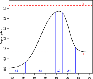
Figure 1: Example of a double logistic function used for projecting the five-year gains in life expectancy, plotted against life expectancy.

2.2 Projecting Mortality and Fertility Rates

The UN’s current method generates assumptions about future age-specific fertility and mortality rates for most countries by projecting forward the overall level of future fertility or mortality, and then converting the overall levels to age-specific rates.

The UN’s current method for projecting life expectancy at birth (hereafter just referred to as life expectancy) for most countries is as follows. Five-year gains in life expectancy for country $c$ in time period $t$, $\ell_{c,t}$, are projected using a deterministic double logistic function, namely,

$$\ell_{c,t+1}=\ell_{c,t}+g\bigl{(}\ell_{c,t}|\bolds{\theta}^{c}\bigr{)},$$ (2)

where five-year gains $g(\ell_{c,t}|\bolds{\theta}^{c})$ are given by

$$g\bigl{(}\ell_{c,t}|\bolds{\theta}^{c}\bigr{)}$$

$$\quad=\frac{k^{c}}{1+\exp(-{A_{1}}(\ell_{ct}-\Delta_{1}^{c}-A_{2}\Delta_{2}^{c})/{\Delta_{2}^{c}})}$$ (3)

$${{\mbox{$\displaystyle\qquad{}+\frac{z^{c}-k^{c}}{1+\exp(-{A_{1}}(\ell_{ct}-\sum_{i=1}^{3}\Delta_{i}^{c}-A_{2}\Delta_{4}^{c})/{\Delta_{4}^{c}})}$}}}.$$

In (2.2), $\bolds{\theta}^{c}=(\Delta_{1}^{c},\Delta_{2}^{c},\Delta_{3}^{c},\Delta_{4}^{c},k^{c},z^{c})$ are the six parameters of the double logistic function for country $c$, whose meaning is illustrated in Figure 1, and $A_{1}$ and $A_{2}$ are constants. The parameters to be used for a given country are chosen by the UN analyst for that country from a list of five predetermined patterns that represent different rates of improvement in life expectancy.

The most used measure of the overall level of fertility is the total fertility rate (TFR) for country $c$ at time $t$, defined as $f_{c,t}=k\sum_{x=1}^{N-1}F_{c,x,t}$, where $F_{c,x,t}$ is the fertility rate in country $c$ for age group $x$ at time $t$. The TFR is the average number of children a woman would bear in her life if exposed to the age-specific fertility rates prevalent at time $t$.

The UN’s current method for projecting TFR takes account of several empirical regularities. The past century has been dominated by the fertility transition, a shift from high fertility and high mortality to low fertility and low mortality, that started in Europe and North America in the late 19th century and in East Asia in the mid 20th century. It has now started in almost all countries and is complete in many (Hirschman (1994)). The patterns of change in different countries have been similar. The TFR starts from a high level that differs among countries but is typically between 4 and 8, and then starts to decline slowly. The pace of decline reaches a peak about half way through the transition. Then the pace of decline slows, stopping some time after the TFR goes below the replacement level of about 2.1 children per woman. In several low-fertility countries, a slow increase has been observed after this point.

The UN has projected five-year decrements in the TFR using a double logistic function, similar to the function used for projecting gains in life expectancy. The parameters to be used for a given country are chosen by the UN analyst for that country from a list of three predetermined patterns. In the projections, the TFR is held constant once it reaches 1.85 children, which represents the deterministic ultimate fertility level or asymptote. For countries where the TFR is below 1.85 at the start of the projection, the TFR is projected to increase by 0.05 children per 5-year period until the ultimate level is reached.

Projected values of the total fertility rate and life expectancy are converted to age-specific fertility and mortality rates based on past patterns or model life tables, and population projections are produced using the cohort component method. Finally, high and low variants are produced by increasing or decreasing the total fertility rate in each future period by half a child.

3 Bayesian Population Projections

The UN’s current projection method does not yield an assessment of uncertainty about future population quantities. It is somewhat subjective because the double logistic functions used have been selected by the analyst from a small number of predetermined possibilities rather than estimated from the data. It is also somewhat rigid in that the set of double logistic functions used is small and may not cover a full range of realistic future possibilities.

To address these issues, we have developed a Bayesian probabilistic population projection method. This involves building Bayesian hierarchical models to project the total fertility rate and life expectancy, each of which produces a large number of possible future trajectories from the posterior predictive distribution. These are then input to the cohort component projection method to provide a posterior predictive distribution of any future population quantity of interest. We now briefly describe the method.

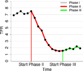
Figure 2: The three phases of the model for total fertility—Phase I: pre-demographic transition; Phase II: fertility transition; Phase III; post-transition recovery.

3.1 Bayesian Fertility Projection Model

We model the typical evolution of a country’s fertility over time as consisting of three phases, shown in Figure 2 (Alkema et al. (2011)). Phase I precedes the beginning of the fertility transition and is characterized by high fertility that is stable or increasing. All countries have now completed this phase, and so it is not of interest for projections; we do not model it further. Phase II consists of the fertility transition during which fertility declines from high levels to below the replacement level of 2.1 children per woman. Phase III is the post-fertility transition period.

To model fertility declines in Phase II, we use a double logistic function, but with some modifications. First, to make the model stochastic, we add a heteroscedastic error term. Second, we allow the parameters $\theta^{(c)}$ to vary continuously rather than being restricted to a small number of possibilities. Third, we model the values of a parameter for different countries as arising from a “world” distribution. This leads to estimates that borrow strength from data for other countries and makes the model hierarchical. This is important because, for a single country, the data are sparse (at most 12 five-year periods for most countries), and estimation of the country-specific double-logistic curve can be unstable, as it involves estimating five parameters from 12 or fewer data points. The hierarchical model stabilizes the estimation.

The resulting model is as follows:

$$f_{c,t+1}=f_{c,t}-r\bigl{(}f_{c,t}|\bolds{\delta}^{c}\bigr{)}+a_{c,t},$$ (4)

where the five-year decrement $r(f_{c,t}|\bolds{\delta}^{c})$ is given by

$$r\bigl{(}f_{c,t}|\bolds{\delta}^{c}\bigr{)}$$

$$\quad=\frac{-d^{c}}{1+\exp(-{2\ln(9)}(f_{c,t}-\sum_{i=2}^{4}\bigtriangledown_{i}^{c}+0.5\bigtriangledown_{1}^{c})/{\bigtriangledown_{1}^{c}})}$$ (5)

$$\qquad{}+\frac{d^{c}}{1+\exp(-{2\ln(9)}(f_{c,t}-\bigtriangledown_{4}^{c}-0.5\bigtriangledown_{3}^{c})/{\bigtriangledown_{3}^{c}})}$$

with $\bolds{\delta}^{c}=(\bigtriangledown_{1}^{c},\bigtriangledown_{2}^{c},\triangle_{3}^{c},\bigtriangledown_{4}^{c},d^{c})$ being a vector of country-specific parameters and $a_{c,t}\stackrel{{\scriptstyle\mathrm{ind}}}{{\sim}}N(0,\sigma(t,\break f_{c,t})^{2})$, where $\sigma(t,f_{c,t})$ is a function that describes how the error standard deviation changes with fertility level and time period.

The country-specific parameters, $\bolds{\delta}_{c}$, are assumed to be drawn from a world distribution whose parameters (or hyperparameters) themselves have a diffuse prior distribution, namely, $\bolds{\delta}_{c}\stackrel{{\scriptstyle\mathrm{i.i.d.}}}{{\sim}}h(\cdot,\bolds{\phi})$, where $\bolds{\phi}\sim p(\bolds{\phi})$. The resulting Bayesian hierarchical model is estimated using Markov chain Monte Carlo.

We define a country as having entered Phase III once two consecutive five-year increases below a TFR of 2 children have occurred. By this definition 21 countries had entered Phase III by 2010: 19 European countries, the USA and Singapore. For these countries, TFR has tended to increase back toward replacement level after they entered Phase II, reversing the secular trend of fertility decline. This is by now a well-documented trend (Myrskyla, Kohler and Billari (2009)).

To model this, we used a single first-order autoregressive model with long-term mean $\mu$ equal to the approximate replacement fertility level of 2.1 for all countries in Phase III, namely,

$$f_{c,t+1}-\mu=\rho(f_{c,t}-\mu)+b_{c,t},$$ (6)

where $b_{c,t}\stackrel{{\scriptstyle\mathrm{i.i.d.}}}{{\sim}}N(0,\sigma_{b}^{2})$. The parameters $\rho$ and $\sigma_{b}$ were estimated by maximum likelihood from the 54 time periods observed in the 21 countries that have entered Phase III, yielding $\hat{\rho}=0.89$ and $\hat{\sigma}_{b}=0.10$. The estimated value of $\rho$ gives expected increases that are similar to the current UN increments of 0.05 children for each five-year period until the TFR equals 1.85.

3.2 Bayesian Life Expectancy Projection Model

We model female life expectancy similarly to Phase II total fertility. We use the UN’s double logistic function to project expected gains, but we add a heteroscedastic error term, we allow the parameters of the country-specific double logistic functions to vary continuously among countries rather than being restricted to five pre-assigned possibilities, and we assume that the double logistic parameters are draws from a common “world” distribution (Raftery et al. (2013)).

The resulting Bayesian model is as follows:

$$\ell_{c,t+1}=\ell_{c,t}+g\bigl{(}\ell_{c,t}|\bolds{\theta}^{(c)}\bigr{)}+e_{c,t},$$ (7)

where

$$g\bigl{(}\ell_{c,t}|\bolds{\theta}^{c}\bigr{)}$$

$$\quad=\frac{k^{c}}{1+\exp(-{A_{1}}(\ell_{ct}-\Delta_{1}^{c}-A_{2}\Delta_{2}^{c})/{\Delta_{2}^{c}})}$$ (8)

$${{\mbox{$\displaystyle\qquad{}+\frac{z^{c}-k^{c}}{1+\exp(-{A_{1}}(\ell_{ct}-\sum_{i=1}^{3}\Delta_{i}^{c}-A_{2}\Delta_{4}^{c})/{\Delta_{4}^{c}})}$}}}.$$

In (3.2), $\bolds{\theta}^{c}=(\Delta_{1}^{c},\Delta_{2}^{c},\Delta_{3}^{c},\Delta_{4}^{c},k^{c},z^{c})$, $e_{c,t}\stackrel{{\scriptstyle\mathrm{ind}}}{{\sim}}N(0,\break\omega(\ell_{c,t})^{2})$, where $\omega(\cdot)$ is a smooth function representing how the error standard deviation depends on the current level of life expectancy, and $A_{1}$ and $A_{2}$ are constants. The country-specific parameters are assumed to be drawn from world distributions, as follows:

$$\quad\Delta_{i}^{c} \stackrel{{\scriptstyle\mathrm{i.i.d.}}}{{\sim}} \mathrm{TN}_{[0,100]}\bigl{(}\Delta_{i},\sigma_{\Delta_{i}}^{2}\bigr{)},\quad i=1,\ldots,4,$$ (9)

$$\quad k^{c} \stackrel{{\scriptstyle\mathrm{i.i.d.}}}{{\sim}} \mathrm{TN}_{[0,10]}\bigl{(}k,\sigma_{k}^{2}\bigr{)},$$ (10)

$$\quad z^{c} \stackrel{{\scriptstyle\mathrm{i.i.d.}}}{{\sim}} \mathrm{TN}_{[0,1.15]}\bigl{(}z,\sigma_{z}^{2}\bigr{)},$$ (11)

where TN${}_{[a,b]}(\mu,\sigma^{2})$ denotes a truncated normal distribution with mean parameter $\mu$ and standard deviation parameter $\sigma$, truncated to lie between $a$ and $b$.

The world hyperparameters on the right-hand sides of equations (9)–(11) are given diffuse prior distributions, with one notable exception, namely, $z$. The country-specific parameter $z^{c}$ is the asymptotic linear increase of life expectancy in country $c$ per five-year period, and this is restricted to be less than 1.15, which is highly informative. This is based on the empirical fact that over the past 170 years the maximum country-specific life expectancy in year $y$ has been increasing highly linearly with $y$ (Oeppen and Vaupel (2002)); 1.15 years per five-year period is the upper bound of a 99.9% confidence interval for the rate of increase. Accordingly, the prior distribution of $z$ is also bounded above by 1.15.

Male life expectancy is highly correlated with female life expectancy and is almost invariably lower. We therefore project female and male life expectancy jointly, by first projecting female life expectancy using the Bayesian hierarchical model described above and then projecting the gap between them. On average, the gap tends to increase as a function of female life expectancy as female life expectancy increases up to about 75 years, and then tends to decrease. It also has extreme values, often corresponding to conflicts when male life expectancy is more affected than female. We represent this using the regression model of Lalic (2011) with $t$-distributed errors for $G_{c,t}$, the gap in country $c$ at time period $t$.

The model is as follows:

$$G_{c,t+1}=\min\bigl{\{}\bigl{(}G^{*}_{c,t+1}\bigr{)}_{+},18\bigr{\}},$$

where

$$G^{*}_{c,t+1} = \cases{\beta_{0}+\beta_{1}\ell_{c,1950-1955}\cr\quad{}+\beta_{2}G_{c,t}+\beta_{3}\ell_{c,t}\cr\quad{}+\beta_{4}(\ell_{c,t}-75)_{+}\cr\quad{}+\epsilon_{c,t},&if $\ell_{c,t}\leq M$,\cr\gamma_{1}G_{c,t}+\epsilon_{c,t},&if $\ell_{c,t}>M$,}$$

$$\epsilon_{c,t} \stackrel{{\scriptstyle\mathrm{i.i.d.}}}{{\sim}} t\bigl{(}\mu=0,\sigma^{2}=0.0665,\nu=2\bigr{)}$$

and $M=86.2$ years, the highest life expectancy recorded in the WPP 2010. The gap is restricted to be no more than 18 years, which is slightly above the highest value observed to date. The model was estimated by maximum likelihood.

3.3 Bayesian Population Projections

The methods just described formed the basis for probabilistic population projections for 159 countries, comprising just under 90% of the world’s population in 2010. The 38 countries with generalized HIV/AIDS epidemics were not included because they have very different mortality patterns and require special treatment. Thirty small countries or areas with populations under 100,000 were also excluded.

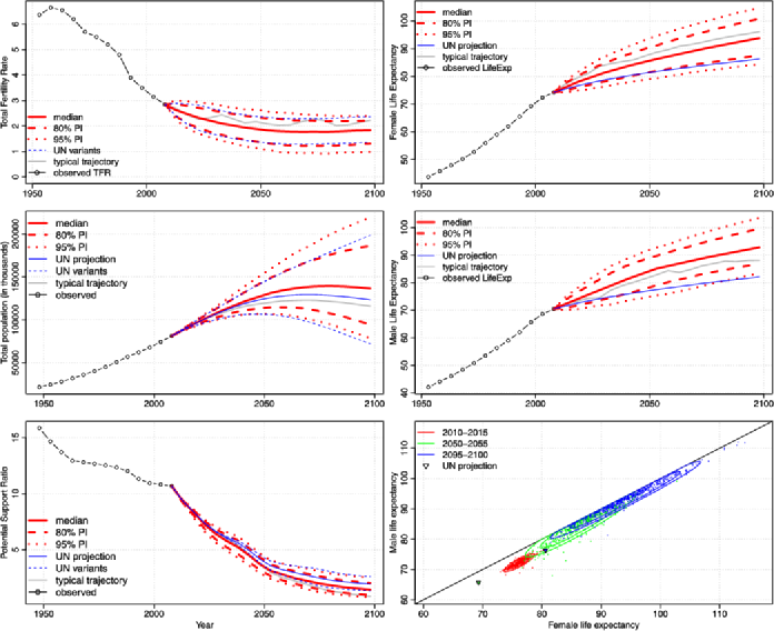
Figure 3: Bayesian probabilistic population projections for Egypt, 2010–2100: major population indicators. Left, top to bottom: total fertility rate; total population; potential support ratio (20–64 population$/$65$+$ population). Right, top to bottom: female life expectancy; male life expectancy; joint predictive distribution of female and male life expectancy for 2010–2015, 2050–2055 and 2095–2100. The Bayesian predictive distributions are shown in red: median—solid; 80% projection interval—dashed; 95% projection interval—dotted. The UN WPP 2010 medium projection is shown as a solid blue line and the UN WPP 2010 high and low projections are shown as dashed blue lines. The solid grey line represents a typical trajectory.

To produce the probabilistic projections, 2000 trajectories of the total fertility rate for each five-year period from 2010 to 2100, and 2000 joint trajectories of female and male life expectancy were simulated from their posterior predictive distributions. These were then converted to age-specific fertility and age- and sex-specific mortality rates using established UN methods, and input to the cohort-component method. Current UN assumptions about future international migration were used. This yielded joint probabilistic projections of any future population quantity of interest.

The method was described in more detail by Raftery et al. (2012), which also reported the results of a study assessing the model by estimating it from data for 1950–1990 and using it to project population for all 159 countries in the 20-year period 1990–2010. The projections of total population, total fertility rate, and female and male life expectancy were reasonably accurate and the projection intervals were reasonably well calibrated.

The results for Egypt are shown in Figure 3. For the total fertility rate, the UN high and low variants turn out to be similar to the limits of the Bayesian pointwise 80% projection intervals. For life expectancy, the current UN projections do not provide any assessment of uncertainty or even scenarios. The Bayesian approach suggests higher future life expectancy, but the current UN projection is within the Bayesian 95% interval for most years. The median Bayesian projection of total population in 2100 is about 10% higher than the UN’s WPP 2010 projection, but this has to be seen in the context of the considerable uncertainty about Egypt’s total population at century’s end. The Bayesian 80% interval for Egypt’s population in 2100 ranges from 96 to 184 million.

Perhaps the most striking result is the projected trend in the potential support ratio, equal to the number of people aged 20–64 per person aged 65 or over. This can be roughly interpreted as the number of workers per retiree and is important, for example, for planning old-age social security systems. In Egypt this is currently 10.7, but is projected to decline dramatically to 1.4 by the end of the century, with an 80% projection interval 1.0–2.0. For context, in the U.S. this is currently 4.6 and is projected to decline to 1.8 by 2100.

This trend is well known for the U.S. and other developed countries (Lee (2011)) and features in political debate and policy making there. What is perhaps surprising is that the same trend is projected for developing countries with young populations and currently high potential support ratios like Egypt. Indeed, the decline is likely to be even steeper in many developing countries than in developed countries. Egypt in 2100 may well have an older population than the U.S. or any other country in the world does now. The projection intervals show that this overall trend is essentially inevitable, even if there is some uncertainty about the extent of the eventual decline.

4 Accommodating Controversy About Ultimate Fertility Level via Bayes

Our method for projecting the total fertility rate for all countries was discussed during a three-day Expert Group Meeting convened by the UN in December 2009 (United Nations Population Division (2009)) and was favorably assessed. The predictive median from our method was then used as the UN’s (deterministic) projection of TFR in the WPP 2010 (United Nations (2011b)). Apart from that, the UN used the same deterministic projection method in WPP 2010 as in WPP 2008 and previous projections, but is considering making future projections probabilistic.

Substantively, this led to projections of a slower decline in fertility in Africa than had previously been expected. It also led to projections of a slow increase in fertility in Europe, which had previously been projected to remain at the sub-replacement level of 1.85 child per woman once it reached this threshold. The previous UN projection in WPP 2008 went up only to 2050 and projected a world population of 9 billion. The new WPP 2010 projection went up to 2100 for the first time and projected a world population of 10 billion, a billion more (although for a longer time horizon).

Overall, the new projections were well received. However, there was one critique, relating not to the statistical method, but to the assumption in the model for TFR in Phase III that asymptotically TFR oscillates around the approximate replacement rate of 2.1, namely, that $\mu=2.1$ in (6).

Basten, Coleman and Gu (2012) argued that the UN’s assumption of an eventual recovery of fertility toward replacement is not justified for five advanced East Asian economies (Korea, Japan, Hong Kong, Singapore and Taiwan). They pointed out that the national statistical agencies of these countries project lower fertility rates than does the UN, that the relevant scientific literature does not suggest an increase in fertility in the short term, that a recent unpublished survey of experts concluded that fertility would not increase as markedly as the UN predicts, and that current evidence about fertility intentions does not suggest an immediate appetite for more children in these countries. They also argued that the UN assumption is based largely on European experience and that there is no reason to assume that it will carry over to East Asia. We interpret their arguments as implying that $\mu$ in (6) may differ between East Asian countries and others, and that for the five East Asian countries they consider, $\mu$ should be less than the replacement level of 2.1.

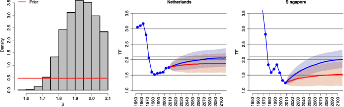
Figure 4: Results for the Bayesian hierarchical model for Phase III fertility (12)–(4): left: posterior distribution of $\bar{\mu}$, the world mean of the country-specific asymptotes. Center and right: projections of the TFR with 80% projection intervals for the Netherlands and Singapore under the WPP 2010 model (6) in blue and the Bayesian hierarchical model for Phase III in red.

We do not necessarily accept this critique, and there are counterarguments. However, here we suggest a possible way to relax the assumptions underlying the Phase III fertility model (6) so as to accommodate the critique and make the model more fully data-based. Instead of requiring every country in Phase III to follow the same model (6), we allow both $\mu$ and $\rho$ to vary between countries following a Bayesian hierarchical model:

$$f_{c,t+1}-\mu_{c}=\rho_{c}(f_{c,t}-\mu_{c})+\varepsilon_{c,t},$$ (12)

where $\varepsilon_{c,t}\stackrel{{\scriptstyle\mathrm{i.i.d.}}}{{\sim}}N(0,\sigma^{2}_{\varepsilon})$ and

$$\mu_{c}\sim TN_{[0,\infty)}\bigl{(}\bar{\mu},\sigma^{2}_{\mu}\bigr{)};\quad\rho_{c}\sim TN_{[0,1]}\bigl{(}\bar{\rho},\sigma^{2}_{\rho}\bigr{)}.$$ (13)

The prior distributions for the hyperparameters are as follows:

$$\bar{\mu} \sim U[0,2.1];\quad\sigma_{\mu}\sim U[0,0.318];$$

$$\bar{\rho} \sim U[0,1];\quad\sigma_{\rho}\sim U[0,0.289];$$ (14)

$$\sigma_{\varepsilon} \sim U[0,0.5].$$

The priors are chosen to be diffuse, except for the prior on $\bar{\mu}$, the world mean of the country-specific asymptotes, which is restricted to be no greater than the replacement level of 2.1. Since the only critiques to date suggest that the UN’s current choice of 2.1 may be too high, this truncation seems to accommodate current expert opinion.

Figure 4 shows some of the results of fitting the Bayesian hierarchical model (12)–(4) to the data from the 21 countries that have entered Phase III. The posterior distribution of $\bar{\mu}$, the world mean of the country-specific TFR asymptotes, essentially excludes values below 1.6. For most of the 21 countries, the projections are similar to those from the WPP 2010 model (6) of Alkema et al. (2011) with fixed $\mu=2.1$; this can be seen, for example, for the Netherlands in the middle panel of Figure 4.

The only one of Basten, Coleman and Gu’s (2012) five advanced East Asian economies that has entered Phase III is Singapore, for which the projections are shown in the left panel of Figure 4. Remarkably, it is also the only one of the 21 Phase III countries for which the projections differ substantially between the $\mu=2.1$ model and the Bayesian hierarchical model with country-specific $\mu_{c}$. The projection under the Bayesian hierarchical model (12)–(4) is much lower than under the previous model (6), as Basten et al. argued it should be. It asymptotes at 1.5 instead of 2.1. This suggests that the data provide some support for Basten et al.’s contention, and also that the proposed Bayesian hierarchical model for Phase III can accommodate differences of this kind among countries.

5 Discussion

We have developed a method for probabilistic population projections for possible use by the United Nations in its biennial projections of the populations of all countries. We have developed Bayesian hierarchical models for projecting future overall levels of fertility and mortality for each country, as measured by the total fertility rate and life expectancy for females and males. Samples from the resulting posterior predictive distributions are converted into age-specific fertility and mortality rates. These are then used as inputs to the cohort component projection method, yielding samples from the posterior predictive distributions of any future population quantity of interest. The method has performed reasonably well in terms of out of sample predictive performance.

The method focuses on the overall levels of fertility and mortality, traditionally viewed as the biggest sources of error in population projections. However, there are other sources of uncertainty not taken into account in our method. These include uncertainty about the base population, sex ratio at birth, age structure of fertility and mortality and also about net international migration, the latter being increasingly important (National Research Council (2000)). Not including these does not seem to have led to substantial miscalibration of the method, but future work should aim to incorporate these other sources of uncertainty. Also, the method is not currently adapted to the countries with generalized HIV/AIDS epidemics which comprise about 10% of the world’s population, and it will be important to extend the method to these countries.

The UN projects populations not only for all countries, but also for regions and other sets of countries including trading blocs and economic, political and ecological groupings (United Nations (2011a)). Aggregation of deterministic projections is straightforward: just add up the projections for the component countries. For probabilistic projections it is not so simple, because between-country correlations have to be taken into account. Our approach treats countries as exchangeable rather than independent, but it does not model the additional correlation that may exist between, for example, contiguous countries. For life expectancy, work to date suggests that our model does account for most of this correlation; there is little correlation between forecast errors (Raftery et al. (2013)). For fertility there may be some excess between-country correlation, and this needs to be accounted for in future work.

Our approach is largely Bayesian, and Bayesian thinking was essential in overcoming the statistical challenges, including the limited amount of data for each country and the differences and similarities among countries in the way fertility and life expectancy have evolved. The Bayesian approach allowed us to borrow strength from other countries through the hierarchical model, thus avoiding instabilities in estimation. It also gave us a way to combine the posterior predictive distributions of fertility and mortality with the cohort component model in a natural way, and to incorporate external information about the asymptotic rate of increase in life expectancy through its prior distribution. In addition, it provided the basis for a way to accommodate Basten, Coleman and Gu’s (2012) critique of the UN’s assumption about the equilibrium distribution of total fertility rate. Fienberg (2011) described several other major governmental and policy problems for which Bayesian thinking proved useful.

We have adopted a fully Bayesian approach, however, only when it led to an improved solution. For example, our model for the female-male gap in life expectancy is not Bayesian, because there are enough data to estimate the model reliably via maximum likelihood. Fully Bayesian estimation of this model would give similar results and would be more complicated, and so did not seem worth doing.

Several other Bayesian approaches to population projection have been proposed, but these have focused mainly on projecting mortality. Girosi and King (2008) proposed a Bayesian method for forecasting age-specific mortality that can incorporate covariates. They showed that for short-term forecasts, their method outperformed the widely used time series method of Lee and Carter (1992) (without covariates) on average for 48 countries with better mortality data. This result, obtained when covariates were used, requires additional data that may not be reliable or even available in many countries. The reliability of their approach remains unproven for medium- or long-term projections due to the reliance on covariates and the difficulties in predicting them beyond a few decades. They did not give probabilistic forecasts, although their method may in principle be able to provide them.

Czado, Delwarde and Denuit (2005) developed a Bayesian method for estimating the Poisson log-bilinear formulation of Brouhns, Denuit and Vermunt’s (2002) version of the Lee-Carter model. Pedroza (2006) proposed a Bayesian approach to the Lee-Carter model by accounting for the uncertainty in the age parameters as well as the mortality index usually forecasted. While the latter two approaches account for uncertainty in the Lee-Carter model, their generalization to all countries is hindered by the nonavailability of age-specific mortality rates. Daponte, Kadane and Wolfson (1997) developed a Bayesian approach to the problem of reconstructing past populations, which is different from the problem of projecting future populations that we address here.

Expert-based probabilistic population projections have been produced by Lutz and colleagues (Lutz, Sanderson and Scherbov, 1998, 2004, 2008). However, this method is not explicitly based on available data, and instead relies on a collection of experts and their ability to specify probabilistic bounds, that may or may not be accurate (Alho and Spencer (2005)). Thus, while like Bayesian approaches this method uses expert knowledge, it does not update it formally using data, and so is not Bayesian in the usual sense.

Our model for the total fertility rate has been adopted by the UN as the basis for its deterministic projections in WPP 2010 (United Nations (2011b)). The UN also issued probabilistic projections using the methods described here on an experimental basis in November 2012, at http://esa.un.org/unpd/ppp. The UN is considering issuing official probabilistic projections for the first time in WPP 2014, using our methods.

The methods described here are implemented in the R packages bayesTFR (Ševčíková, Alkema and Raftery (2011)), bayesLife (Ševčíková and Raftery (2011)), bayesPop (Ševčíková and Raftery (2012)) and bayesDem (Ševčíková (2011)).

References

- Alho and Spencer (2005) {bbook}[mr] \bauthor\bsnmAlho, \bfnmJuha M.\binitsJ. M. and \bauthor\bsnmSpencer, \bfnmBruce D.\binitsB. D. (\byear2005). \btitleStatistical Demography and Forecasting. \bpublisherSpringer, \blocationNew York. \bidmr=2171856 \bptokimsref \endbibitem
- Alkema et al. (2011) {barticle}[auto:STB—2013/03/04—13:35:07] \bauthor\bsnmAlkema, \bfnmL.\binitsL., \bauthor\bsnmRaftery, \bfnmA. E.\binitsA. E., \bauthor\bsnmGerland, \bfnmP.\binitsP., \bauthor\bsnmClark, \bfnmS. J.\binitsS. J., \bauthor\bsnmPelletier, \bfnmF.\binitsF., \bauthor\bsnmBuettner, \bfnmT.\binitsT. and \bauthor\bsnmHeilig, \bfnmG. K.\binitsG. K. (\byear2011). \btitleProbabilistic projections of the total fertility rate for all countries. \bjournalDemography \bvolume48 \bpages815–839. \bptokimsref \endbibitem