Effective ergodicity in single-spin-flip dynamics

Abstract

A quantitative measure of convergence to effective ergodicity, Thirumalai-Mountain (TM) metric, is applied to Metropolis and Glauber single spin flip dynamics. In computing this measure, finite lattice ensemble averages are obtained using the exact solution for one dimensional Ising model, where as, the time averages are computed with Monte Carlo simulations. The time evolution of effective ergodic convergence of Ising magnetization is monitored. By this approach, diffusion regimes of the effective ergodic convergence of magnetization are identified for different lattice sizes, non-zero temperature and non-zero external field values. Results show that caution should be taken using TM metric at system parameters that give rise to strong correlations.

I Introduction

Cooperative phenomena are present in many different fields [1]. A unifying approach in studying cooperation among individual units emerge as a mathematical model that most resembles the nature of the problem. The first and the most successful of these models which were exactly solvable was the one dimensional Ising model, a closed chain of $n$ cooperating units, mimicking spins in ferromagnetic materials [2, 3, 4]. Time dependent statistics of the Ising model has been studied in depth before [5, 6], where single flip dynamics on $n$ spins is introduced by changing a single spin’s value with an associated transition probability. Natural consequence of generating such dynamics in a given statistical ensemble is the question of how and when the system behaves ergodically, i.e., ensemble averages being equivalent to the time averages. This question is not only interesting due to fulfilling Boltzmann’s equilibrium statistical mechanics [7, 8, 9], but for its crucial importance in practical applications, such as, in simple liquids [10, 11], assessing quality of the Monte Carlo simulations [12], earthquake fault networks [13, 14] and in econophysics [15]. Most of these studies address the problem of identifying ergodic or non-ergodic regimes. In this study, we investigate the time evolution of the rate of effective ergodic convergence under different system parameters to identify its so called diffusion regimes.

The Ising model and its analytic solution for the finite size total magnetization corresponding to the ensemble average are introduced in Sec. II. In Sec. III we will provide details of our strategy of computing time averages using Metropolis and Glauber single spin dynamics defined on the Ising model. In Sec. IV we briefly review the basic definitions of ergodicity from applied statistical mechanics point of view. The mathematical literature based on measure theory is largely ignored. However, a quantitative measure for the identification of effective ergodic dynamic is needed. In Sec. V the fluctuation metric [10, 16] is adapted for Ising model’s total magnetization. By this approach, the rate of effective ergodic convergence of magnetization is monitored in single spin flip dynamics. We report the diffusion behavior of the ergodic convergence and identify different regimes depending on different lattice sizes, temperature and external field values in Sec. VI.

II The Ising model

Consider a one dimensional lattice that contains $N$ sites. Each site’s value can be labelled as $\{s_{i}\}_{i=1}^{N}$. In the two state version of the lattice, which is the Ising model [2, 3, 4], sites can take up two values, such as $\{1,-1\}$. These values correspond to spin up and spin down states, for example as a model of magnetic material or the state of a neuron [17].

The total energy, Hamiltonian of the system can be written as follows

$$\mathcal{H}(\{s_{i}\}_{i=1}^{N},J,H) = J\Big{(}(\sum_{i=1}^{N-1}s_{i}s_{i+1})+(s_{1}s_{N})\Big{)}$$ (1)

$$+H\sum_{1}^{N}s_{i}.$$

This expression contains two interactions, one due to nearest-neighbors (NN) and one due to an external field. Note that, additional term in NN interactions $s_{1}s_{N}$ term appears due to periodic or cyclic boundary conditions to provide translational invariance. Coefficients $J$ and $H$ corresponds to scaling of these interactions respectively. A reduced form is used in Eq.(1) using the unit thermal background, using the Boltzmann factor $\beta=\frac{1}{k_{B}T}$,

$$K=\beta J,\qquad h=\beta H.$$ (2)

The partition function for this system can be written by using the transfer matrix technique [4]

$$Z_{N}=Tr\big{(}V^{N}\big{)}.$$ (3)

$V$ is the transfer matrix defined as follows

$$V=\begin{pmatrix}e^{K+h}&e^{-K}\\ e^{-K}&e^{K-h}\end{pmatrix}.$$ (4)

The resulting free energy for the finite system appears in terms of eigenvalues of the transfer matrix, $\lambda_{1}$ and $\lambda_{2}$ [4]

$$Z_{N} = \lambda_{1}^{N}+\lambda_{2}^{N},$$ (5)

$$\lambda_{1,2} = e^{K}\big{[}\cosh{h}\pm\sqrt{\sin^{2}h+e^{-4K}}\big{]}.$$ (6)

The canonical free energy for the finite system is defined as follows [4]

$$f(N,T,h) = -k_{B}T\frac{1}{N}lnZ_{N},$$ (7)

$$\frac{1}{N}lnZ_{N} = ln\lambda_{1}+\frac{1}{N}ln\big{[}1+(\lambda_{2}/\lambda_{1})^{N}\big{]}.$$ (8)

We are interested in finite size total magnetization, to compute the ensemble average of it, $M_{E}(N,\beta,H)$, analytically. Differentiating canonical free energy with respect to $H$ will yield a long expression for $M_{E}$,

$$M_{E}(N,\beta,H) = \big{(}NM_{1}M_{2}^{N-1}+NM_{3}M_{4}^{N-1}\big{)}/M_{5},$$ (9)

$$M_{1} = {{\beta\,\cosh\left(H\,\beta\right)\,\sinh\left(H\,\beta\right)}\over{\sqrt{e^{-4\,\beta\,J}+\sinh^{2}\left(H\,\beta\right)}}}+\beta\,\sinh\left(H\,\beta\right),$$

$$M_{2} = \sqrt{e^{-4\,\beta\,J}+\sinh^{2}\left(H\,\beta\right)}+\cosh\left(h\,\beta\right),$$

$$M_{3} = -M_{1}+2\beta\,\sinh\left(H\,\beta\right),$$

$$M_{4} = -M_{2}+2\cosh\left(H\,\beta\right),$$

$$M_{5} = \big{(}\sqrt{e^{-4\,\beta\,J}+\sinh^{2}\left(H\,\beta\right)}+\cosh\left(H\,\beta\right)\big{)}^{N}$$

$$+\big{(}\cosh\left(H\,\beta\right)-\sqrt{e^{-4\,\beta\,J}+\sinh^{2}\left(H\,\beta\right)}\big{)}^{N}.$$

Note that in Eq.(9), the Boltzmann factor is explicitly written. Further explorations of the analytical solutions are beyond the scope of this study.

III Metropolis and Glauber single spin flip dynamics

One of the ways to generate dynamics for a lattice system similar to Ising model in a computer simulation is changing the value of a randomly chosen site to its opposite value. This procedure is called single spin flip dynamics in the context of Monte Carlo simulations [6]. However, the quality of this kind of dynamics depends highly on the quality of the random number generator (RNG) [18, 19] we employ in selecting the site to be flipped. However, we gather that Marsenne-Twister as an RNG [20] is sufficiently good for this purpose.

In generating such a dynamics, there is an associated transition probability in the single spin flip. This probability would determine if the flip introduced by the Monte Carlo procedure is an acceptable physical move. Two forms of transition probability can be used that correspond to Boltzmann density. The following expressions generate Glauber and Metropolis dynamics respectively,

$$p_{Glauber}(\{s_{i}\}_{i=1}^{N}) = \exp(-\beta\Delta\mathcal{H})/\big{(}1+\exp(-\beta\Delta\mathcal{H})\big{)},$$ (10)

$$= 1/\big{(}1+\exp(\beta\Delta\mathcal{H})\big{)},$$

$$p_{Metropolis}(\{s_{i}\}_{i=1}^{N}) = min\big{(}1,\exp(-\beta\Delta\mathcal{H})\big{)}.$$ (11)

where $\Delta\mathcal{H}$ is the total energy difference between single spin flipped and non-flipped configurations. The resulting transition probability is compared against a randomly generated number $r$, where $r\in[0,1]$. The move is accepted if the transition probability is smaller then $r$. This procedure, generally known as Metropolis-Hastings Monte Carlo, samples the canonical ensemble [6].

IV Ergodicity

Boltzmann made the hypothesis that the solution of any dynamical system, its trajectories, will evolve in time over phase-space regions where macroscopic properties are close to the thermodynamic equilibrium [9]. Consequently, ensemble averages and time averages will yield the same measure in thermodynamic equilibrium. A form of this hypothesis states that average values of an observable $g$ over its ensemble of accessible state points, namely ensemble averaged value can be recovered by time averaged values of the observable’s time evolution, $g(t)$ from $t_{0}$ to $t_{N}$,

$$\langle g\rangle=lim_{t_{N}\to\infty}\int_{t_{0}}^{t_{N}}g(t)dt,$$ (12)

where $\langle\rangle$ indicates ensemble averaged value. Note that, the definition of ergodicity is not uniform in the literature [21, 10, 22]. Some works require that system should visit all accessible states in the phase-space to reach ergodic behavior. This is seldomly true. And considering the fact that coarse graining of phase-space occurs, most of the accessible state values are clustered. Frequently, effective ergodicity can be reached if the system uniformly samples the coarse-grained regions relatively quickly [10].

Conditions of ergodicity in the transition states, a stochastic matrix of transition probabilities, generated by spin flip dynamics is studied in the context of Markov chains [22, 23]. This type of ergodicity implies that any state can be reached from any other. The Monte Carlo procedure explained above may be ergodic by construction in this sense for long enough times.

V Concept of Ergodic Convergence

A quantitative measure of effective ergodic convergence relies on the fact that identical components of the system, particles or a discrete sites, carry identical average characteristics at thermal equilibrium [10]. Hence, effective ergodic convergence, $\Omega_{G}(t)$, can be quantified over time for an observable, a property, $g$. Essentially it can be computed as a difference the between ensemble averaged value of $g$ and the sum of the instantaneous values of $g$ for each of the components. This is termed Thirumalai-Mountain (TM) $G$-fluctuating metric [10, 16], expressed as follows at a given time $t_{k}$

$$\Omega_{G}(t_{k})=\frac{1}{N}\sum_{j=1}^{N}\big{[}g_{j}(t_{k})-\langle g(t_{k})\rangle\big{]}^{2},$$ (13)

where $g_{j}(t_{k})$ is the time-averaged per component and $\langle g(t_{k})\rangle$ is the instantaneous ensemble average defined as

$$g_{j}(t_{k}) = \frac{1}{k}\sum_{i=0}^{k}g_{j}(t_{i}),$$ (14)

$$\langle g(t_{k})\rangle = \frac{1}{N}\sum_{j=1}^{N}g_{j}(t_{k}).$$ (15)

Hence the rate of ergodic convergence is measured with

$$\Omega_{G}^{{}^{\prime}}=\frac{\Omega_{G}(t)}{\Omega_{G}(0)}\to\frac{1}{tD_{G}}$$ (16)

where $D_{G}$ is the property’s diffusion coefficient and $\Omega_{G}$ effective ergodic convergence. If $1/\Omega_{G}^{{}^{\prime}}$ is linear in time, any point in phase-space is said to be equally likely. This approach is used in simple liquids [10, 11], and earthquake fault networks [13, 14].

We would like to investigate the behavior of $1/\Omega_{G}^{{}^{\prime}}$ for the Ising model. The adaption of the $\Omega_{G}$ for total magnetization at time $t_{k}$ as a function of temperature and external field values reads

$$\Omega_{M}(t_{k},N,\beta,h) = \big{[}M_{T}(t_{k})-M_{E}\big{]}^{2},$$ (17)

$$M_{T} = \frac{1}{k}\sum_{i=0}^{k}M(t_{i}),$$

where $M_{T}(N,\beta,h)$ and $M_{E}(N,\beta,h)$ correspond to time and ensemble averaged total magnetization. Note that the value of $M_{E}(N,\beta,h)$ is fixed and is computed using the analytical solutions given in Sec. II, where as $M_{T}(N,\beta,h)$ is computed in the course of Metropolis or Glauber dynamics. Here we slightly differ in comparison to the TM approach and use constant ensemble average, because in our case the value of the ensemble average is available in exact form as given in Eq.(9).

VI Diffusion Regimes

We have identified the time evolution of the effective ergodic convergence measure, $\Omega_{M}(t_{k},N,\beta,h)$, for the total magnetization of a one dimensional Ising model. Depending on which transition probability is used for the acceptance criterion, we generate Metropolis and Glauber single spin flip dynamics for the following model parameters: number of spin sites $N=\{32,64,128,256,512\}$, Boltzmann factor $\beta=\{0.5,1.0\}$ and non-zero external field values $H=\{0.50,1.0\}$ with setting short-range interaction strength to $J=1.0$ for all cases [24]. We generate a dynamics up to half a million Monte Carlo steps for all combination of parameters, hence the maximum $k$. At the rejected moves, rejected single spin flip configurations, the value of $\Omega_{M}(t_{k},N,\beta,h)$ is set to the previous accepted value. We did not use external field values and temperatures close to zero, because total magnetization’s exact solution fails for zero temperature. In the case of zero external field, total magnetization is zero and Monte Carlo relaxation time is long.

We have generated a set of time evolutions of the effective ergodic convergence measure combined in three different schemes: varying external fields, increasing number of spin sites and different temperature values. For better statistics, $512$ spin sites are used for the variation of external fields and temperatures. By employing such a combination scheme, we could judge the relations among the variation of different parameters in the behavior of the ergodic convergence measure over time. The Monte Carlo steps play a role of pseudo-dynamical time.

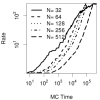
(a)

(b)

Figure 1: Inverse effective ergodic convergence in Glauber dynamics with different system sizes with fixed temperature $\beta=1.0$ and external fields $H=\{0.5,1.0\}$ at (a) and (b) respectively.

(a)

(b)

Figure 2: Inverse effective ergodic convergence in Metropolis dynamics with different system sizes with fixed temperature $\beta=1.0$ and external fields $H=\{0.5,1.0\}$ at (a) and (b) respectively.

To be able to judge the diffusion behavior of the time evolutions of the effective ergodic convergence measure, we used the following expression with $D_{M}$, the diffusion coefficient,

$$1/\Omega_{M}^{{}^{\prime}}=\frac{\Omega_{M}(t_{0},N,\beta,h)}{\Omega_{M}(t_{k},N,\beta,h)} \to tD_{M}.$$ (19)

We call this value so called inverse effective ergodic convergence rate, simply the rate. The rate in our plots shows an increasing value over time. A higher value implies that the system is closer to ergodic regime.

Figures 1(a), 1(b) and Figures 2(a), 2(b) show the effect of the lattice size, different number of spin sites, two different external field values at fixed unit thermal background, for Glauber and Metropolis dynamics respectively. It is seen in all cases that smaller size leads to faster ergodic convergence. This behavior is more pronounced with the Glauber dynamics. It is well known that Glauber dynamics provides faster convergence to equilibrium [6]. When the external field is higher, at $1.0$, we observe two different diffusion regimes. Those regimes can be clearly judged from inflection points given on the rate curves. Those inflection points, plateau regions, are significant in the Glauber dynamics. Again, the plateau regions are shifted for smaller size configurations to the left of the figure, due to faster convergence we mentioned.

(a)

(b)

Figure 3: Effective ergodic convergence in Glauber dynamics with different external field values with fixed size $N=512$ and temperature $\beta=\{0.5,1.0\}$ at (a) and (b) respectively.

For varying external field values, there is only a single diffusion regime for low external field values. However upon increasing of the field values we again observe inflection point in the rate curves. This signifies two different diffusion regimes for the rate. This is demonstrated in Figure 3(a) and 3(b).

(a)

(b)

Figure 4: Effective ergodic convergence in Glauber dynamics with different temperatures with fixed size $N=512$ and external fields $H=\{0.5,1.0\}$ at (a) and (b) respectively.

Temperature dependence of the rate curve is shown in Figure 4(a) and 4(b). We see that combination of higher temperature and external field values induce a change in the diffusion behavior. We observe that plateau regions become larger upon increasing temperature.

VII Summary

The behavior of the rate of convergence to ergodicity is characterized for the Ising model using the modified Thirumalai-Mountain (TM) metric for the total magnetization. We aimed at determining the rate’s behavior over time. We conclude that combination of stronger temperature or external field values generates a regime change in the ergodic convergence. Hence, caution should be taken using TM metric at system parameters that give rise to strong correlations.

References

- [1] G. H. Wannier. The statistical problem in cooperative phenomena. Rev. Mod. Phys., 17:50–60, Jan 1945.
- [2] Ernst Ising. Beitrag zur theorie des ferromagnetismus. Zeitschrift für Physik A Hadrons and Nuclei, 31(1):253–258, 1925.
- [3] Stephen G Brush. History of the lenz-ising model. Reviews of Modern Physics, 39(4):883, 1967.
- [4] RJ Baxter. Exactly solvable models in statistical mechanics. Academic Press London, 1982.
- [5] Roy J Glauber. Time-dependent statistics of the ising model. Journal of Mathematical Physics, 4(2):294–307, 1963.
- [6] Kurt Binder and Dieter W Heermann. Monte Carlo simulation in statistical physics: an introduction. Springer, 2010.
- [7] R. C. Tolman. The Principles of Statistical Mechanics. Oxford University Press, New York, 1938.
- [8] I. E. Farquhar. Ergodic Theory in Statistical Mechanics. Interscience Publishers, Inc, New York, 1964.
- [9] Jay Robert Dorfman. An introduction to chaos in nonequilibrium statistical mechanics. Number 14. Cambridge University Press, 1999.
- [10] Raymond D Mountain and D Thirumalai. Measures of effective ergodic convergence in liquids. The Journal of Physical Chemistry, 93(19):6975–6979, 1989.
- [11] Vanessa K de Souza and David J Wales. Diagnosing broken ergodicity using an energy fluctuation metric. The Journal of Chemical Physics, 123(13):134504, 2005.
- [12] JP Neirotti, David L Freeman, and JD Doll. Approach to ergodicity in monte carlo simulations. Physical Review E, 62(5):7445, 2000.
- [13] KF Tiampo, JB Rundle, W Klein, JS Sá Martins, and CD Ferguson. Ergodic dynamics in a natural threshold system. Physical Review Letters, 91(23):238501–238501, 2003.
- [14] KF Tiampo, JB Rundle, W Klein, J Holliday, JS Sá Martins, and CD Ferguson. Ergodicity in natural earthquake fault networks. Physical Review E, 75(6):066107, 2007.
- [15] Ole Peters. Optimal leverage from non-ergodicity. Quantitative Finance, 11(11):1593–1602, 2011.
- [16] D. Thirumalai, R.D. Mountain, and T.R. Kirkpatrick. Ergodic behavior in supercooled liquids and in glasses. Physical Review A, 39(7):3563, 1989.
- [17] John J Hopfield. Neural networks and physical systems with emergent collective computational abilities. Proceedings of the national academy of sciences, 79(8):2554–2558, 1982.
- [18] Aaldert Compagner. Definition of randomness. American Journal of Physics, 59(8):700, 1991.
- [19] Wolfhard Janke. Pseudo random numbers: Generation and quality checks. Lecture Notes John von Neumann Institute for Computing, 10:447, 2002.
- [20] M. Matsumoto and T. Nishimura. Mersenne twister: A 623-dimensionally equidistributed uniform pseudo-random number generator. ACM Transactions on Modeling and Computer Simulation, 8(1):3–30, 1998.
- [21] SK Ma. Statistical mechanics. World Scientific, Singapore, 1985.
- [22] JFC Kingman. The ergodic behaviour of random walks. Biometrika, pages 391–396, 1961.
- [23] AG Pakes. Some conditions for ergodicity and recurrence of markov chains. Operations Research, 17(6):1058–1061, 1969.
- [24] M. Süzen. isingLenzMC: Monte Carlo for classical Ising Model, 2014. v0.2 http://cran.r-project.org/web/packages/isingLenzMC/index.html.