The Kearns–Saul inequality for Bernoulli and Poisson-binomial distributions

Abstract.

We give a direct rigorous proof of the Kearns–Saul inequality which bounds the Laplace transform of a generalised Bernoulli random variable. We extend the arguments to generalised Poisson-binomial distributions and characterise the set of parameters such that an analogous inequality holds for the sum of two generalised Bernoulli random variables.

1. Introduction and main results

A generalised Bernoulli random variable $X\sim\mathrm{Ber}(p)$ with parameter $p\in[0,1]$ is defined by its distribution function $\mathbf{P}(X=1-p)=1-\mathbf{P}(X=-p)=p$. It differs from a classical Bernoulli random variable in that it is shifted so as to have mean zero. In [3] the Laplace transform $\mathbf{E}\mathrm{e}^{tX}$ of a generalised Bernoulli random variable $X\sim\mathrm{Ber}(p)$ was bounded by

$$p\mathrm{e}^{t(1-p)}+(1-p)\mathrm{e}^{-tp}\leqslant\exp\left[\frac{1-2p}{4\log[(1-p)/p]}t^{2}\right],\quad t\in\mathbb{R},\quad 0\leqslant p\leqslant 1.$$ (1.1)

A rigorous proof of this inequality was provided in [1], where the function

$$g_{p}(t)=\frac{1}{t^{2}}\log\left[p\mathrm{e}^{t(1-p)}+(1-p)\mathrm{e}^{-tp}\right],\quad t\in\mathbb{R},$$ (1.2)

was analysed using convexity arguments. In the same paper, the task of proving that the function $g_{p}$ is strictly unimodal with a unique maximum at $t=t_{p}^{\ast}=2\log[(1-p)/p]$ was classified as an ”intriguing open problem”. Here, a differentiable real-valued function $f$ on $\mathbb{R}$ is said to be strictly unimodal if there exists an $x$ such that the derivative $f^{\prime}$ is positive on $(-\infty,x)$ and negative on $(x,\infty)$. In the next section we provide a proof of the following solution to this problem.

Theorem 1.1.

For every $p\in[0,1]$, the function $g_{p}$ defined in Eq. 1.2 is strictly unimodal.

A natural extension of generalised Bernoulli random variables is the family of Poisson-binomial distributions [2]. For a positive integer $n$ and a parameter vector $\mathbf{p}=(p_{1},\ldots,p_{n})\in[0,1]^{n}$, the $\mathrm{PoiBin}_{n}(\mathbf{p})$ distribution is defined as the distribution of the random variable $X_{1}+\ldots+X_{n}$, where the $X_{i}\sim\mathrm{Ber}(p_{i})$ are independent generalised Bernoulli random variables. In the following we will be interested in the case $n=2$ and provide a generalisation of Eq. 1.1. The statement and proof of this generalisation, as well as Corollary 1.4, are the main results of this paper. The analogue of the function $g_{p}$, defined in Eq. 1.2, which occupies a central role in the proof of the Kearns–Saul inequality, is

$$g_{p_{1},p_{2}}(t)=g_{p_{1}}(t)+g_{p_{2}}(t)=\frac{1}{t^{2}}\log\left[\mathrm{e}^{-t(p_{1}+p_{2})}\left(1+p_{1}\left(\mathrm{e}^{t}-1\right)\right)\left(1+p_{2}\left(\mathrm{e}^{t}-1\right)\right)\right].$$ (1.3)

By $\langle x,y\rangle$ we denote an ordered pair of real numbers $x$ and $y$.

Theorem 1.2.

Let $g_{p_{1},p_{2}}$ be the function defined in Eq. 1.3 and

$$t_{p_{1},p_{2}}^{\ast}=\log\left[\frac{1-p_{1}}{p_{1}}\frac{1-p_{2}}{p_{2}}\right].$$ (1.4)

Then $g_{p_{1},p_{2}}\left(t_{p_{1},p_{2}}^{\ast}\right)=0$ and there exist sets $C\subset B\subset A\subset[0,1]^{2}$ such that

1. $g_{p_{1},p_{2}}^{\prime}(t)$ is positive for $t<0$ if and only if $\langle p_{1},p_{2}\rangle\in A$;

2. $g_{p_{1},p_{2}}^{\prime}(t)$ is negative for $t>t_{p_{1},p_{2}}^{\ast}$ if and only if $\langle p_{1},p_{2}\rangle\in B$;

3. $g_{p_{1},p_{2}}^{\prime}(t)$ is positive for $0<t<t_{p_{1},p_{2}}^{\ast}$ if and only if $\langle p_{1},p_{2}\rangle\in C$.

In particular, $g_{p_{1},p_{2}}$ is unimodal if and only if $\langle p_{1},p_{2}\rangle\in C$.

The closed, convex sets $A$ and $B$ are given explicitly by Eqs. 3.3 and 3.7. The boundary of the set $C$ can be determined numerically by solving the differential equation 3.10. The following result gives an explicit sufficient condition for $g_{p_{1},p_{2}}$ to be unimodal.

Theorem 1.3.

A sufficient condition for $g_{p_{1},p_{2}}$ to be unimodal is $\langle p_{1},p_{2}\rangle\in D$, where

$$D=\left\{\langle p_{1},p_{2}\rangle\in[0,1]^{2}:12p_{1}p_{2}\left(p_{1}p_{2}+p_{1}+p_{2}\right)-14p_{1}p_{2}+p_{1}^{2}+p_{2}^{2}\leqslant 0\right\}$$ (1.5)

is a closed convex subset of $C$.

The sets $A$, $B$, $C$ and $D$ are depicted in Fig. 1. One can see that $B\backslash D$ is fairly small and that the inclusion $D\subset C\subset B$ thus contains a considerable amount of information about the shape of $C$. As a corollary to Theorem 1.2 we obtain the following result, a direct generalisation of the Kearns–Saul inequality for Poisson-binomial random variables.

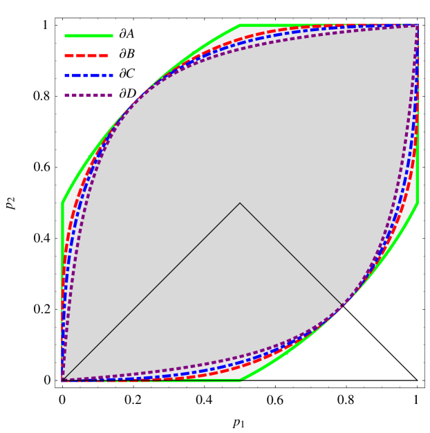
Figure 1. Illustration of the sets appearing in Theorem 1.2 about the behaviour of the function $g_{p_{1},p_{2}}$ (defined in Eq. 1.3) in different regions of the parameter space $[0,1]^{2}$. For $\langle p_{1},p_{2}\rangle\in A$, the region with the green solid boundary, the derivative $g_{p_{1},p_{2}}^{\prime}$ is positive on the interval $\left(-\infty,0\right)$. For $\langle p_{1},p_{2}\rangle\in B$, the region with the red dot-dashed boundary, the derivative $g_{p_{1},p_{2}}^{\prime}$ is negative on the interval $\left(t_{p_{1},p_{2}}^{\ast},\infty\right)$. For $\langle p_{1},p_{2}\rangle\in C$, the region with the blue dash-dotted boundary, the derivative $g_{p_{1},p_{2}}^{\prime}$ is positive on the interval $\left(0,t_{p_{1},p_{2}}^{\ast}\right)$. For $\langle p_{1},p_{2}\rangle\in D$, the region with the purple dotted boundary, the function $g_{p_{1},p_{2}}$ has only two inflection points and is unimodal by Theorem 1.3. The triangular region $\Delta$, to which attention is restricted in the proof of Theorem 1.2, is bounded by black lines.

Corollary 1.4.

For every $\langle p_{1},p_{2}\rangle\in C\subset[0,1]^{2}$, the Laplace transform of the generalised Poisson-binomial random variable $X\sim\mathrm{PoiBin}_{2}(p_{1},p_{2})$ satisfies

$$\mathbf{E}\mathrm{e}^{tX}\leqslant\exp\left[\frac{1-p_{1}-p_{2}}{\log[(1-p_{1})/p_{1}(1-p_{2})/p_{2}]}t^{2}\right],\quad t\in\mathbb{R}.$$ (1.6)

Proof.

The distribution function of a $\mathrm{PoiBin}_{2}(p_{1},p_{2})$-distributed random variable $X$ is given by

$$\mathbf{P}(X=-p_{1}-p_{2})= (1-p_{1})(1-p_{2}),$$

$$\mathbf{P}(X=1-p_{1}-p_{2})= p_{1}(1-p_{2})+(1-p_{1})p_{2},$$

$$\mathbf{P}(X=2-p_{1}-p_{2})= p_{1}p_{2},$$

and its Laplace transform therefore takes the form

$$\mathbf{E}\mathrm{e}^{tX}= (1-p_{1})(1-p_{2})\mathrm{e}^{-t(p_{1}+p_{2})}+(p_{1}+p_{2}-2p_{1}p_{2})\mathrm{e}^{t(1-p_{1}-p_{2})}+p_{1}p_{2}\mathrm{e}^{t(2-p_{1}-p_{2})}$$

$$= \mathrm{e}^{-t(p_{1}+p_{2})}\left[1+p_{1}\left(e^{t}-1\right)\right]\left[1+p_{2}\left(e^{t}-1\right)\right]$$

$$= \exp\left[t^{2}g_{p_{1},p_{2}}(t)\right].$$

Theorem 1.2 implies that, for $\langle p_{1},p_{2}\rangle\in C$, the function $g_{p_{1},p_{2}}$ has a unique maximum at $t=t_{p_{1},p_{2}}^{\ast}$, and therefore satisfies

$$g_{p_{1},p_{2}}(t)\leqslant g_{p_{1},p_{2}}\left(t_{p_{1},p_{2}}^{\ast}\right)=\frac{1-p_{1}-p_{2}}{\log[(1-p_{1})/p_{1}(1-p_{2})/p_{2}]},\quad t\in\mathbb{R}.$$ (1.7)

The claim follows. ∎

We conclude this section with a some remarks and open problems. We have seen that the sets $A$, $B$ and $D$ are convex and from Fig. 1 it appears that the same true for the set $C$.

Problem 1.

Show that the set $C$ appearing in the statement of Theorem 1.2 is convex.

Based on numerical computations, we conjecture that inequality 1.6 does, in fact, hold for a parameter region $C^{\prime}$ slightly larger than $C$, even though $g_{p_{1},p_{2}}$ would not be unimodal for $\langle p_{1},p_{2}\rangle\in C^{\prime}\backslash C$.

Problem 2.

Characterise the set of parameters $\langle p_{1},p_{2}\rangle$ such that inequality 1.6 holds.

An extension of our results to $\mathrm{PoiBin}_{n}$-distributions with $n$ larger than two appears to be very difficult. One reason is that, as $n$ increases, the number of critical points of the analogue of the function $g_{p_{1},p_{2}}$ increases and we do not know, in general, how to find the abscissa of the critical point corresponding to the global maximum.

2. Proof for generalised Bernoulli random variables

In this section we prove Theorem 1.1 about the unimodality of the function $g_{p}$, defined in Eq. 1.2. In the following, by unimodality, concavity and convexity, we always mean strict unimodality, strict concavity and strict convexity. The derivative of the function $g_{p}$ is given by

$$g_{p}^{\prime}(t)=\frac{(1-p)pt\left(\mathrm{e}^{t}-1\right)-2\left(1+p\left(\mathrm{e}^{t}-1\right)\right)\log\left[\mathrm{e}^{-pt}\left(1+p\left(\mathrm{e}^{t}-1\right)\right)\right]}{\left(1+p\left(\mathrm{e}^{t}-1\right)\right)t^{3}},$$

and $g_{p}^{\prime}(t)$ vanishes for $t=t_{p}^{\ast}=2\log[(1-p)/p]$. In order to prove unimodality we will, without loss of generality, assume that $p$ is less than $1/2$ and $t_{p}^{\ast}$ thus positive. If $p>1/2$, one may consider instead the random variable $-X$, which is $\mathrm{Ber}(1-p)$-distributed. The boundary case $p=1/2$ is best dealt with separately: in this case the function $g_{1/2}$ is symmetrical with a maximum at $t=0$, and is easily seen to be unimodal. We first record the following easy properties of the function $f_{p}:t\mapsto t^{3}g_{p}^{\prime}(t)$ for later reference.

Lemma 2.1.

For every $p<1/2$, the function $f_{p}$ has exactly two inflection points; their abscissas are $t=0$ and $t=t_{p}^{\ast}/2=\log[(1-p)/p]$. The function $f_{p}$ is concave on $\mathbb{R}^{-}\cup\left(t_{p}^{\ast}/2,\infty\right)$ and convex on $\left(0,t_{p}^{\ast}/2\right)$.

Proof.

To prove the lemma, we first compute the second derivative of $f_{p}$ which equals

$$f_{p}^{\prime\prime}(t)=\frac{p(1-p)t\mathrm{e}^{t}(1-p-p\mathrm{e}^{t})}{\left(1+p\left(\mathrm{e}^{t}-1\right)\right)^{3}}.$$

This expression vanishes exactly for $t=0$ and $t=t_{p}^{\ast}/2$. To conclude that these are indeed the abscissas of reflection points we need to verify that the third derivative of $f_{p}$ does not vanish there. We find that $f_{p}^{(3)}(0)=p(1-p)(1-2p)$ and $f_{p}^{(3)}\left(t_{p}^{\ast}/2\right)=\log[p/(1-p)]/8$, which are manifestly positive and negative, respectively, for $p<1/2$. ∎

We can now give a proof of our first main result.

Proof of Theorem 1.1.

We will show that $g_{p}^{\prime}(t)$ is positive for $t<t_{p}^{\ast}$ and negative for $t>t_{p}^{\ast}$ by analysing the sign of $f_{p}(t)=t^{3}g_{p}^{\prime}(t)$ in the three intervals $\left(-\infty,0\right)$, $\left(0,t_{p}^{\ast}\right)$ and $\left(t_{p}^{\ast},\infty\right)$. We first show that $f_{p}(t)<0$ for $t<0$. Since $f_{p}$ itself as well as its first derivative vanish at $t=0$, the claim follows from the concavity of $f_{p}$ on $\mathbb{R}^{-}$. We next show that $f_{p}(t)<0$ for $t>t_{p}^{\ast}$. Since $f_{p}\left(t_{p}^{\ast}\right)=0$ it suffices by the concavity of $f_{p}$ on $\left(t_{p}^{\ast},\infty\right)$ to show that

$$\mathfrak{r}(p)\coloneqq f_{p}^{\prime}\left(t_{p}^{\ast}\right)=2p-1+2(1-p)p\log[(1-p)/p]$$

is negative for $p<1/2$. This follows from the observation that $\mathfrak{r}$ is monotonely increasing with derivative $\mathfrak{r}^{\prime}(p)=2(1-2p)\log[(1-p)/p]>0$ and the fact that $\mathfrak{r}(1/2)=0$. Lastly, we verify that $f_{p}(t)>0$ for $0<t<t_{p}^{\ast}$. This is a direct consequence of the facts that $f_{p}(0)=f_{p}^{\prime}(0)=f_{p}^{\prime\prime}(0)=0$, $f_{p}^{(3)}(0)>0$, $f_{p}\left(t_{p}^{\ast}\right)=0$, $f_{p}^{\prime}\left(t_{p}^{\ast}\right)<0$, and that $f_{p}$ has exactly one inflection point in the interval $\left(0,t_{p}^{\ast}\right)$. ∎

3. Proof in the Poisson-Binomial case

In this section we extend the previous arguments to the case of Poisson-binomial random variables. The derivative of the function $g_{p_{1},p_{2}}$ defined in Eq. 1.3 is given by

$$g_{p_{1},p_{2}}^{\prime}(t)= g_{p_{1}}^{\prime}(t)+g_{p_{2}}^{\prime}(t)$$

$$= \frac{1}{t^{3}}\left\{t\left[2+p_{1}+p_{2}-\frac{1-p_{1}}{1-p_{1}\left(1-\mathrm{e}^{t}\right)}-\frac{1-p_{2}}{1-p_{2}\left(1-\mathrm{e}^{t}\right)}\right]\right.$$

$$\left.\qquad-2\log\left[\left(1-p_{1}\left(1-\mathrm{e}^{t}\right)\right)\left(1-p_{2}\left(1-\mathrm{e}^{t}\right)\right)\right]\right\},$$

and this expression vanishes for $t=t_{p_{1},p_{2}}^{\ast}=\log((1-p_{1})/p_{1}(1-p_{2})/p_{2})$. In order to prove unimodality we will, without loss of generality, assume that $p_{1}+p_{2}$ is less than or equal to one and $t^{\ast}$ thus non-negative, and that $p_{1}\geqslant p_{2}$. This can always be guaranteed by considering $-X_{i}$ instead of $X_{i}$ and/or renaming the variables $X_{1}$, $X_{2}$. We thus concentrate on the triangular region $\left\{\langle p_{1},p_{2}\rangle:p_{2}\leqslant(p_{1},1-p_{1})^{-}\right\}$ in the parameter space $[0,1]^{2}$. Here and in the following, $(x,y)^{-}$ denotes the minimum of two real numbers $x$ and $y$. As before, the boundary cases $p_{2}=(p_{1},1-p_{1})^{-}$ are dealt with first. Instead of $g_{p_{1},p_{2}}$ we will often analyse the function $f_{p_{1},p_{2}}:t\mapsto t^{3}g_{p_{1},p_{2}}^{\prime}(t)$ which is better behaved at $t=0$. We also introduce the notation $p^{\pm}=(3\pm\sqrt{3})/6$.

Lemma 3.1.

The function $f_{p_{1},(p_{1},1-p_{1})^{-}}$ has the following properties.

1. If $p_{1}<1/2$, then $f_{p_{1},p_{1}}$ has roots at $t=0$ and $t=t_{p_{1},p_{1}}^{*}$, and is negative on $\left(-\infty,0\right)\cup\left(t_{p_{1},p_{1}}^{*},\infty\right)$ and positive on $\left(0,t_{p_{1},p_{1}}^{*}\right)$.

2. If $p_{1}\in\left[1/2,p^{+}\right]$, then $f_{p_{1},1-p_{1}}$ is symmetrical, has a root at $t=0$, and is negative on $\mathbb{R}\backslash\{0\}$.

3. If $p_{1}>p^{+}$, then $f_{p_{1},1-p_{1}}$ is symmetrical and has a root at $t=0$. Moreover, there exists $t_{p_{1}}^{\dagger}>0$ such that $f_{p_{1},1-p_{1}}\left(\pm t_{p_{1}}^{\dagger}\right)$ vanishes and $f_{p_{1},1-p_{1}}$ is negative on $\left(-\infty,-t_{p_{1}}^{\dagger}\right)\cup\left(t_{p_{1}}^{\dagger},\infty\right)$ and positive on $\left(-t_{p_{1}}^{\dagger},t_{p_{1}}^{\dagger}\right)\backslash\{0\}$.

In particular, the function $g_{p_{1},(p_{1},1-p_{1})^{-}}$ is strictly unimodal if and only if $p_{1}\leqslant p^{+}$.

Proof.

The first statement follows from Theorem 1.1 and the observations that $g_{p,p}=2g_{p}$ and $t_{p,p}^{\ast}=t_{p}^{\ast}$. For assertion ii) we observe that $f_{p_{1},1-p_{1}}$ is manifestly symmetrical and that its second derivative is, up to positive factors, a polynomial of degree two, namely

$$f_{p_{1},1-p_{1}}^{\prime\prime}(t)=\frac{p_{1}(1-p_{1})t\mathrm{e}^{t}\left(\mathrm{e}^{2t}-1\right)}{\left[1+p_{1}\left(\mathrm{e}^{t}-1\right)\right]^{3}\left[1+(1-p_{1})\left(\mathrm{e}^{t}-1\right)\right]^{3}}\mathfrak{p}_{p_{1}}\left(\mathrm{e}^{t}\right),$$

where $\mathfrak{p}_{p_{1}}(x)=-p_{1}(1-p_{1})\left[1-2p_{1}(1-p_{1})\right](1+x^{2})+\left[1-4p_{1}(1-2p_{1}^{2}+p_{1}^{3})\right]x$. Since the discriminant of this polynomial is equal to $(1-2p_{1})^{2}[1+2p_{1}(1-p_{1})][1-6p_{1}(1-p_{1})]$, it does not have any real roots if $1/2\leqslant p_{1}<p^{+}$. A quick computation shows that $f_{p_{1},1-p_{1}}$ itself as well as its first three derivatives vanish at $t=0$, and that $f_{p_{1},1-p_{1}}^{(4)}=4p_{1}(1-p_{1})[1-6p_{1}(1-p_{1})]$; this implies the claim for $p_{1}$ strictly less than $p^{+}$. For $p_{1}=p^{+}$ one checks that the only root of $\mathfrak{p}_{p_{1}}$ is equal to zero, which does not correspond to a zero of $\mathfrak{p}_{p^{+}}\left(\mathrm{e}^{t}\right)$. Moreover, the first-non-vanishing derivative of $f_{p^{+},1-p+}$ at zero (the sixth!) is equal to $-8/9$, proving the claim. We now turn to the proof of iii). If $p_{1}$ exceeds $p^{+}$, then the fourth derivative of $f_{p_{1},1-p_{1}}$ at $t=0$ is positive, and the two roots $x_{p_{1}}^{\pm}$ of $\mathfrak{p}_{p_{1}}$ correspond to the abscissas $t_{p_{1}}^{\pm}=\log x_{p_{1}}^{\pm}$ of the only two inflection points of $f_{p_{1},1-p_{1}}$. To complete the proof it only remains to check that $f_{p_{1},1-p_{1}}^{(3)}\left(t_{p_{1}}^{\pm}\right)$ is positive and negative, respectively; the lengthy details are omitted. ∎

We now return to the general case and denote by $\Delta$ the triangle $\left\{\langle p_{1},p_{2}\rangle\in[0,1]^{2}:p_{2}<(p_{1},1-p_{1})^{-}\right\}$. As in the generalised Bernoulli case, a large part of the proof of Theorem 1.2 hinges on the convexity properties of the function $f_{p_{1},p_{2}}$. For the statement of the next result we introduce the notation

$$\mathcal{D}(p_{1},p_{2})=12p_{1}p_{2}\left(p_{1}p_{2}+p_{1}+p_{2}\right)-14p_{1}p_{2}+p_{1}^{2}+p_{2}^{2},$$ (3.1)

and

$$\mathcal{A}(p_{1},p_{2})=2p_{1}p_{2}-p_{1}(2p_{1}-1)-p_{2}(2p_{2}-1),$$ (3.2)

which will also be used later on. We will also use the fact that the inclusion

$$D\subset A,\quad D=\left\{\mathcal{D}(p_{1},p_{2})\leqslant 0\right\},\quad A=\left\{\mathcal{A}(p_{1},p_{2})\geqslant 0\right\},$$ (3.3)

holds, which follows from simple algebra.

Lemma 3.2.

For every $\langle p_{1},p_{2}\rangle\in\Delta$, the function $f_{p_{1},p_{2}}$ has two inflection points with abscissas $t=0$ and $t=t_{p_{1},p_{2}}^{\ast}/2$.

1. If $\mathcal{D}(p_{1},p_{2})$ is negative or zero, then these are the only inflection points and $f_{p_{1},p_{2}}$ is concave on $\left(-\infty,0\right)\cup\left(t_{p_{1},p_{2}}^{\ast}/2,+\infty\right)$ and convex on $\left(0,t_{p_{1},p_{2}}^{\ast}/2\right)$.

2. If $\mathcal{D}(p_{1},p_{2})$ is positive and $\mathcal{A}(p_{1},p_{2})$ is zero, then the point $\left(t_{p_{1},p_{2}}^{*},0\right)$ is an additional inflection point of $f_{p_{1},p_{2}}$ and there are no others.

3. if $\mathcal{D}(p_{1},p_{2})$ is positive and $\mathcal{A}(p_{1},p_{2})$ is non-zero, then there exist two additional inflection points with abscissas $t_{p_{1},p_{2}}^{\pm}$.

   1. if $\mathcal{A}(p_{1},p_{2})$ is negative, then $t_{p_{1},p_{2}}^{-}<0$ and $t_{p_{1},p_{2}}^{+}>t_{p_{1},p_{2}}^{\ast}$, and $f_{p_{1},p_{2}}$ is concave on $\left(-\infty,t_{p_{1},p_{2}}^{-}\right)\cup\left(0,t_{p_{1},p_{2}}^{\ast}/2\right)\cup\left(t_{p_{1},p_{2}}^{+},+\infty\right)$ and convex on $\left(t_{p_{1},p_{2}}^{-},0\right)\cup\left(t_{p_{1},p_{2}}^{\ast}/2,t_{p_{1},p_{2}}^{+}\right)$.

   2. if $\mathcal{A}(p_{1},p_{2})$ is positive, then $0<t_{p_{1},p_{2}}^{-}<t_{p_{1},p_{2}}^{\ast}/2$ and $t_{p_{1},p_{2}}^{\ast}/2<t_{p_{1},p_{2}}^{+}<t_{p_{1},p_{2}}^{\ast}$, and $f_{p_{1},p_{2}}$ is concave on $\left(-\infty,0\right)\cup\left(t_{p_{1},p_{2}}^{-},t_{p_{1},p_{2}}^{\ast}/2\right)\cup\left(t_{p_{1},p_{2}}^{+},+\infty\right)$ and convex on $\left(0,t_{p_{1},p_{2}}^{-}\right)\cup\left(t_{p_{1},p_{2}}^{\ast}/2,t_{p_{1},p_{2}}^{+}\right)$.

Proof.

Direct calculation shows that the second derivative of $f_{p_{1},p_{2}}$ vanishes for $t=0$ and $t=t_{p_{1},p_{2}}^{\ast}/2$ and that $f_{p_{1},p_{2}}^{\prime\prime}(t)$ itself can be written as

$$f_{p_{1},p_{2}}^{\prime\prime}(t)=\frac{t\mathrm{e}^{t}\left[p_{1}+p_{2}-1+p_{1}p_{2}\left(\mathrm{e}^{2t}-1\right)\right]}{\left[1+p_{1}\left(\mathrm{e}^{t}-1\right)\right]^{3}\left[1+p_{2}\left(\mathrm{e}^{t}-1\right)\right]^{3}}\mathfrak{p}_{p_{1},p_{2}}\left(\mathrm{e}^{t}\right),$$

where

$$\mathfrak{p}_{p_{1},p_{2}}(x)= (1-p_{1})(1-p_{2})(2p_{1}p_{2}-p_{1}-p_{2})$$

$$+\left[4p_{1}p_{2}(p_{1}+p_{2}-p_{1}p_{2})-6p_{1}p_{2}+p_{1}^{2}+p_{2}^{2}\right]x$$

$$+p_{1}p_{2}\left[2p_{1}p_{2}-p_{1}-p_{2}\right]x^{2}$$

is a polynomial of degree two. For the existence of at least one additional inflection point it is thus necessary that the discriminant $\mathcal{D}(p_{1},p_{2})$ of $\mathfrak{p}_{p_{1},p_{2}}$, which is given by Eq. 3.1, is non-negative. If the discriminant is zero, however, the only real root of the polynomial $\mathfrak{p}_{p_{1},p_{2}}$ equals $\exp\left\{t_{p_{1},p_{2}}^{*}/2\right\}$, which we we have found before, and so no additional inflection point exists in this case; this proves part i).

If $\mathcal{D}(p_{1},p_{2})$ is positive, the roots of $\mathfrak{p}_{p_{1}p_{2}}$ are given by

$$x_{p_{1},p_{2}}^{\pm}=\frac{4p_{1}p_{2}\left(p_{1}+p_{2}-p_{1}p_{2}\right)-6p_{1}p_{2}+p_{1}^{2}+p_{2}^{2}\pm(p_{1}-p_{2})\sqrt{\mathcal{D}(p_{1},p_{2})}}{2p_{1}p_{2}\left(p_{1}+p_{2}-2p_{1}p_{2}\right)}.$$

It is not difficult to check that $x_{p_{1},p_{2}}^{-}$, and hence $x_{p_{1},p_{2}}^{+}>x_{p_{1},p_{2}}^{-}$, are never negative; the roots $x_{p_{1},p_{2}}^{\pm}$ thus correspond to roots $t_{p_{1},p_{2}}^{\pm}=\log x_{p_{1},p_{2}}^{\pm}$ of $\mathfrak{p}_{p_{1},p_{2}}\left(\mathrm{e}^{t}\right)$ and thus to potential inflection points of $f_{p_{1},p_{2}}$. To obtain a complete picture of the convexity properties of $f_{p_{1},p_{2}}$ we will next analyse where the inflection points with abscissas $t_{p_{1},p_{2}}^{\pm}$ are located relative to $t=0$ and $t=t_{p_{1},p_{2}}^{\ast}/2$. After some more algebra we obtain that $t_{p_{1},p_{2}}^{-}$ and $t_{p_{1},p_{2}}^{+}$ lie to either side of $t_{p_{1},p_{2}}^{\ast}/2$. We further find that $\mathcal{A}(p_{1},p_{2})<0$ is equivalent to $t_{p_{1},p_{2}}^{-}$ being negative and $t_{p_{1},p_{2}}^{+}$ exceeding $t_{p_{1},p_{2}}^{\ast}$ (proving iii)iii-a)), that $\mathcal{A}(p_{1},p_{2})>0$ is equivalent to $t_{p_{1},p_{2}}^{-}$ being positive and $t_{p_{1},p_{2}}^{+}$ deceeding $t_{p_{1},p_{2}}^{\ast}$ (proving iii)iii-b)), and finally that $\mathcal{A}(p_{1},p_{2})=0$ implies $t_{p_{1},p_{2}}^{-}=0$ and $t_{p_{1},p_{2}}^{+}=t_{p_{1},p_{2}}^{\ast}$ (proving ii)).

To complete the proof it remains to check the sign of the third derivative of $f_{p_{1},p_{2}}$ at the (maximal) four inflection points; details of these straightforward computations are again omitted. ∎

Typical graphs of $t\mapsto f_{p_{1},p_{2}}(t)$ for different values of $\langle p_{1},p_{2}\rangle$, illustrating the convexity properties obtained in Lemma 3.2, are depicted in Fig. 3. In particular, part i) is illustrated in Figs. 3(i) and 3(j); part ii) in Fig. 3(c); part iii)iii-a) in Fig. 3(b); and part iii)iii-b) in Figs. 3(d), 3(e), 3(f), 3(g) and 3(h).

As in the generalised Bernoulli case we will establish necessary and sufficient conditions for $g_{p_{1},p_{2}}$ to be unimodal by analysing the sign of the function $f_{p_{1},p_{2}}$ on the three intervals $\left(-\infty,0\right)$, $\left(0,t_{p_{1},p_{2}}^{\ast}\right)$ and $\left(t_{p_{1},p_{2}}^{\ast},\infty\right)$, which is done in Propositions 3.3, 3.4 and 3.6 below.

Proposition 3.3.

For every $\langle p_{1},p_{2}\rangle\in\Delta$ the following are equivalent:

1. the derivative of the function $g_{p_{1},p_{2}}$ is positive on $\mathbb{R}^{-}$;

2. the third derivative of $f_{p_{1},p_{2}}$ is non-negative at $t=0$;

3. $p_{1}<p^{+}$ and $p_{2}\geqslant\alpha(p_{1})$, where $\alpha:[0,p^{+}]\to[0,p^{-}]$ is defined by

   $$\alpha(p_{1})=\max{\left\{0,\frac{1}{4}\left[1+2p_{1}-\sqrt{1+12p(1-p)}\right]\right\}}.$$ (3.4)

Proof.

In order to show that i) implies ii), we observe that, for $t<0$, $g_{p_{1},p_{2}}^{\prime}(t)$ being positive is equivalent to $f_{p_{1},p_{2}}(t)$ being negative. Since all three of $f_{p_{1},p_{2}}(0)$, $f_{p_{1},p_{2}}^{\prime}(0)$ and $f_{p_{1},p_{2}}^{\prime\prime}(0)$ are equal to zero, this implies that $f_{p_{1},p_{2}}^{(3)}(0)$ is non-negative. The equivalence between ii) and iii) follows from the fact that

$$f_{p_{1},p_{2}}^{(3)}(0)=p_{1}(1-p_{1})(1-2p_{1})+p_{2}(1-p_{2})(1-2p_{2})=(1-p_{1}-p_{2})\mathcal{A}(p_{1},p_{2})$$

and an easy computation. Finally, for $\langle p_{1},p_{2}\rangle$ such that $p_{2}\geqslant\alpha(p_{1})$ and $\mathcal{A}(p_{1},p_{2})$ thus non-negative, Lemma 3.2 shows that the function $f_{p_{1},p_{2}}$ is concave on $\mathbb{R}^{-}$. In conjunction with the fact that $f_{p_{1},p_{2}}(0)=f_{p_{1},p_{2}}^{\prime}(0)=0$, implies that $f_{p_{1},p_{2}}(t)$ is negative for $t<0$, and thus proves i). ∎

The condition $p_{2}\geqslant\alpha(p_{1})$, together with analogous inequalities for $p_{1}+p_{2}>1$ and $p_{1}<p_{2}$, is an alternative characterisation of the set $A$ from Eq. 3.3 that features in the statement of Theorem 1.2. Since the function $\alpha$ is convex and $\alpha^{\prime}\left(p^{+}\right)$ is equal to one, the set $A$ is convex.

The next result gives a necessary and sufficient condition for the derivative of $g_{p_{1},p_{2}}$ to be negative on the interval $\left(t_{p_{1},p_{2}}^{\ast},\infty\right)$.

Proposition 3.4.

For every $\langle p_{1},p_{2}\rangle\in\Delta$, the following are equivalent:

1. the derivative of the function $g_{p_{1},p_{2}}$ is negative for $t>t_{p_{1},p_{2}}^{\ast}$;

2. the first derivative of $f_{p_{1},p_{2}}$ is non-positive at $t=t_{p_{1},p_{2}}^{\ast}$;

3. $p_{1}<p^{+}$ and $p_{2}\geqslant\beta(p_{1})$, where $\alpha(p_{1})<\beta(p_{1})<(p_{1},1-p_{1})^{-}$ is the unique solution to

   $$\log\left[\frac{1-p_{1}}{p_{1}}\frac{1-\beta(p_{1})}{\beta(p_{1})}\right]=\frac{2(1-p_{1}-\beta(p_{1}))}{p_{1}(1-p_{1})+\beta(p_{1})(1-\beta(p_{1}))}.$$ (3.5)

Proof.

We recall that the negativity of $g_{p_{1},p_{2}}^{\prime}$ on $\left(t_{p_{1},p_{2}}^{\ast},\infty\right)$ is equivalent to the negativity of $f_{p_{1},p_{2}}$ on that interval. As in the proof of Proposition 3.3 we thus see that i) implies ii) because $f_{p_{1},p_{2}}$ vanishes at $t=t_{p_{1},p_{2}}^{\ast}$. We next prove the equivalence of ii) and iii). Direct calculation informs us that

$$h_{p_{1}}(p_{2})\coloneqq \frac{f_{p_{1},p_{2}}^{\prime}\left(t_{p_{1},p_{2}}^{\ast}\right)}{p_{1}(1-p_{1})+p_{2}(1-p_{2})}$$

$$= \log\left[\frac{1-p_{1}}{p_{1}}\frac{1-p_{2}}{p_{2}}\right]-\frac{2(1-p_{1}-p_{2})}{p_{1}(1-p_{1})+p_{2}(1-p_{2})}$$

and

$$\frac{\mathrm{d}}{\mathrm{d}p_{2}}h_{p_{1}}(p_{2})= -\frac{(1-p_{1}-p_{2})^{2}}{p_{2}(1-p_{2})\left[p_{1}(1-p_{1})+p_{2}(1-p_{2})\right]^{2}}\mathfrak{q}_{p_{1}}(p_{2}),$$

where $\mathfrak{q}_{p_{1}}(x)=p_{1}^{2}-2(1+p_{1})p_{2}+3p_{2}^{2}$ is a polynomial of degree two. We will show that, for each $p_{1}\in\left(0,p^{+}\right)$, the function $h_{p_{1}}$ has a unique root $\beta(p_{1})<(p_{1},1-p_{1})^{-}$ and that $h_{p_{1}}(p_{2})$ is positive for $p_{2}<\beta(p_{1})$ and negative for $p_{2}>\beta(p_{1})$. To this end we first observe that $\lim_{p_{2}\to 0}h_{p_{1}}(p_{2})=+\infty$ and $\lim_{p_{2}\to 0}h_{p_{1}}^{\prime}(p_{2})=-\infty$ and that the derivative $h_{p_{1}}^{\prime}$ is, up to positive factors, a quadratic polynomial in $p_{2}$. For $p_{1}<1/2$, the upper boundary of $\Delta$ is given by $p_{2}=p_{1}$ and we thus compute

$$h_{p_{1}}(p_{1})=2\log\left[\frac{1-p_{1}}{p_{1}}\right]-\frac{1-2p_{1}}{p_{1}(1-p_{1})},\quad h_{p_{1}}^{\prime}(p_{1})=\frac{(1-2p_{1})^{2}}{2p_{1}^{2}(1-p_{1})^{2}}.$$

The former expression is negative because it vanishes for $p_{1}=1/2$ and has a positive $p_{1}$-derivative equal to $(1-2p_{1})^{2}/[p_{1}(1-p_{1})]^{2}$; the latter expression is manifestly positive. The existence of a unique root $\beta(p_{1})$ with the claimed property thus follows from the intermediate value theorem. For $p_{1}>1/2$ the upper boundary is given by $p_{2}=1-p_{1}$; in this case we compute

$$h_{p_{1}}(1-p_{1})=h_{p_{1}}^{\prime}(1-p_{1})=h_{p_{1}}^{\prime\prime}(1-p_{1})=0,\quad h_{p_{1}}^{(3)}(1-p_{1})=-\frac{1-6p_{1}(1-p_{1})}{2\left[p_{1}(1-p_{1})\right]^{3}}.$$

If $p_{1}$ is less than $p^{+}$, the last expression is positive and the intermediate value theorem guarantees the existence of a unique root $\beta(p_{1})$ as before. If $p_{1}$ exceeds $p^{+}$, there is no such root. To see this, it is enough to compute the smallest stationary point of the function $p_{2}\mapsto\mathfrak{q}_{p_{1}}(p_{2})$, which is given by $x=\left(1+p_{1}+\sqrt{2p_{1}(1-p_{1})+1}\right)/3$. and observe that it exceeds $1-p_{1}$ if and only if $p_{1}$ is greater than $p^{+}$. The claim that $\beta(p_{1})$ exceeds $\alpha(p_{1})$ follows from the fact that $h_{p_{1}}(\alpha(p_{1}))$ is positive for $0<p_{1}<p^{+}$, which is a tedious, but not difficult, calculation, the details of which we omit.

Lastly, we prove the implication $\lx@cref{refnum}{prop-step2new-2}\wedge\lx@cref{refnum}{prop-step2new-3}\Rightarrow\lx@cref{refnum}{prop-step2new-1}$: if $p_{2}\geqslant\beta(p_{1})>\alpha(p_{1})$, then Lemma 3.2 implies that the function $f_{p_{1},p_{2}}$ is concave on $\left(t_{p_{1},p_{2}}^{\ast},\infty\right)$, Thus the negativity of the first derivative $f_{p_{1},p_{2}}^{\prime}\left(t_{p_{1},p_{2}}^{\ast}\right)$, in conjunction with the fact that the value $f_{p_{1},p_{2}}\left(t_{p_{1},p_{2}}^{\ast}\right)$ is zero, implies that $f_{p_{1},p_{2}}(t)$, and hence $g_{p_{1},p_{2}}^{\prime}(t)$, are negative for $t$ exceeding $t_{p_{1},p_{2}}^{\ast}$. ∎

One checks directly that an explicit parametrisation of the graph of $\beta$ is given by

$$\mathfrak{b}:\mathbb{R}^{+}\to\Delta;\quad\tau\mapsto j(\tau)\left(\begin{array}[]{c}1\\ 1\end{array}\right)+\sqrt{-\partial_{\tau}j(\tau)}\left(\begin{array}[]{c}1\\ -1\end{array}\right);\quad j(\tau)=\frac{1}{\tau}-\frac{1}{\mathrm{e}^{\tau}-1},$$ (3.6)

and that $\mathfrak{b}(t)$ is a saddle point of the function $\langle p_{1},p_{2}\rangle\mapsto f_{p_{1},p_{2}}(t)$. In particular, letting $\tau\to 0$, we find that $\beta\left(p^{+}\right)=p^{-}$. The parametrisation can also be used to show that $\beta$ is monotonely increasing and convex. The inequality $p_{2}\geqslant\beta(p_{1})$, together with analogous inequalities for $p_{1}+p_{2}>1$ and $p_{1}<p_{2}$ define the set $B$ from the statement of Theorem 1.2. Equivalently,

$$B=\left\{\langle p_{1},p_{2}\rangle\in[0,1]^{2}:\left|\log\left(\frac{1-p_{1}}{p_{1}}\frac{1-p_{2}}{p_{2}}\right)\right|\leqslant\frac{2|1-p_{1}-p_{2}|}{p_{1}(1-p_{1})+p_{2}(1-p_{2})}\right\}.$$ (3.7)

The fact that $\beta(p_{1})$ exceeds $\alpha(p_{1})$ for all $p_{1}\in\left(0,p^{+}\right)$ translates directly into the inclusion $B\subset A$. The set $B$ is convex because the function $\beta$ is convex and $\beta^{\prime}\left(p^{+}\right)=1$.

It remains to analyse the interval $\left(0,t_{p_{1},p_{2}}^{\ast}\right)$. Before we prove, in Proposition 3.6, that there exists a function $\gamma$ such that $f_{p_{1},p_{2}}$ is positive on that interval if and only if $p_{2}>\gamma(p_{1})$, we give a proof of Theorem 1.3.

Proof of Theorem 1.3.

The intersection of the triangular region $\Delta$ with the set $D$ defined in Eq. 3.3 can be described as $\left\{\langle p_{1},p_{2}\rangle\in[0,1]^{2}:p_{1}<p^{+}\wedge p_{2}\geqslant\delta(p_{1})\right\}$, where $\delta:\left[0,p^{+}\right]\to\left[0,p^{-}\right]$ is defined by

$$\delta(p_{1})=\frac{\left(7-4\sqrt{3}\right)p_{1}-\left(6-\sqrt{3}\right)p_{1}^{2}}{1+12p_{1}(1-p_{1})}.$$ (3.8)

Similarly to $\alpha$ and $\beta$ the function $\delta$ is convex and satisfies $\delta^{\prime}\left(p^{+}\right)=1$ which implies that the set $D$ is convex. The inclusion $D\subset B$ is thus equivalent to $\delta(p_{1})>\beta(p_{1})$; as in the proof of Proposition 3.4 this can be shown by verifying that $h_{p_{1}}(\delta(p_{1}))$ is negative for all $p_{1}\in\left(0,p^{+}\right)$. For $\langle p_{1},p_{2}\rangle\in D\subset B\subset A$, the negativity of $g_{p_{1},p_{2}}$ on $\left(-\infty,0\right)$ thus follows from Proposition 3.3; the positivity of $g_{p_{1},p_{2}}$ on $\left(t_{p_{1},p_{2}}^{\ast},+\infty\right)$ follows from Proposition 3.4. To see that $g_{p_{1},p_{2}}$ is positive on the interval $\left(0,t_{p_{1},p_{2}}^{\ast}\right)$ it suffices to recall that $f_{p_{1},p_{2}}$ vanishes at $t=0$ and $t=t_{p_{1},p_{2}}^{\ast}$, that the first non-zero derivative of $f_{p_{1},p_{2}}$ at these points is positive and negative respectively, and that $f_{p_{1},p_{2}}$ is convex in-between (Lemma 3.2). ∎

In the next lemma we analyse how the sign of $f_{p_{1},p_{2}}(t)$ varies when $t$ and $p_{1}$ are held fixed and $p_{2}$ changes. We introduce the notations $p_{t}=1/[1+\exp(t/2)]$ and $\langle u(t),v(t)\rangle=\mathfrak{b}(t)$, defined in Eq. 3.6. The notation is illustrated in Fig. 2.

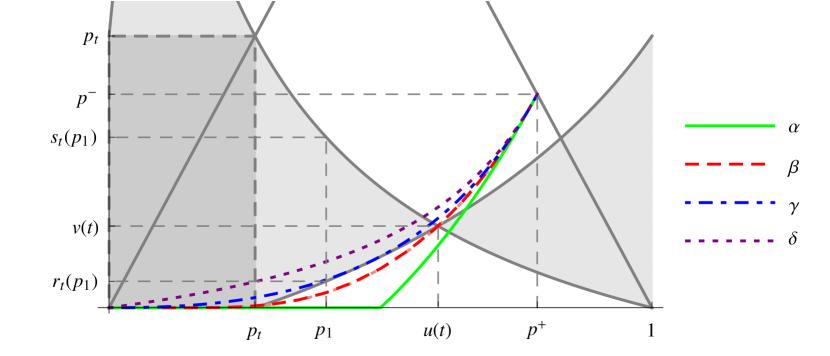
Figure 2. Illustration of the notation used in Lemmas 3.5 and 3.6. The shaded region represents the set $\{f_{p_{1},p_{2}}(t)>0\}$. The solid green curve is the graph of the function $\alpha$ defined in Eq. 3.4 and represents the boundary for $g_{p_{1},p_{2}}^{\prime}(t)$ to be positive for $t<0$. The red dashed curve, visualising the function $\beta$ defined parametrically in Eq. 3.6, represents the boundary for $g_{p_{1},p_{2}}^{\prime}(t)$ to be negative for $t>t_{p_{1},p_{2}}^{\ast}$. The blue dash-dotted curve represents the boundary for $g_{p_{1},p_{2}}^{\prime}(t)$ to be positive for $0<t<t_{p_{1},p_{2}}^{\ast}$ and is derived from Eq. 3.10. The purple line is the graph of the function $\delta$, defined in Eq. 3.8; it represents the boundary for $f_{p_{1},p_{2}}$ to have exactly two inflection points.
The value of $p_{1}$ is $0.4$, the value of $t=2$.

Lemma 3.5.

For every $t>0$, the function $\langle p_{1},p_{2}\rangle\mapsto f_{p_{1},p_{2}}(t)$ has the the following properties:

1. if $p_{1}<p_{t}$, then $f_{p_{1},p_{2}}(t)$ is positive for all $p_{2}\in\left(0,(p_{1},-1p_{1})^{-}\right)$;

2. if $p_{t}\leqslant p_{1}<u(t)$, then there exist $0<r_{t}(p_{1})<s_{t}(p_{1})<(p_{1},1-p_{1})^{-}$ such that $f_{p_{1},p_{2}}(t)$ is negative for $p_{2}\in\left(0,r_{t}(p_{1})\right)$; positive for $p_{2}\in\left(r_{t}(p_{1}),s_{t}(p_{1})\right)$; and negative for $p_{2}\in\left(s_{t}(p_{1}),(p_{1},1-p_{1})^{-}\right)$. The larger boundary point $s_{t}(p_{1})$ satisfies $t^{\ast}_{p_{1},s_{t}(p_{1})}=t$ which is equivalent to

   $$s_{t}(p_{1})=\frac{1-p_{1}}{1+p_{1}\left(\mathrm{e}^{t}-1\right)};$$ (3.9)

Proof.

To establish i) we will prove the slightly stronger claim that $\langle p_{1},p_{2}\rangle\mapsto f_{p_{1},p_{2}}(t)$ is positive on the open square $\left(0,p_{t}\right)^{2}$. We first show that, if $p_{1}<p_{t}$, then $f_{p_{1},p_{2}}(t)$ is positive for $p_{2}=0$ and $p_{2}=p_{t}$. To see that $f_{p_{1},0}(t)$ is positive for $0<p_{1}<p_{t}$, we observe that it vanishes for $p_{1}=0$ and $p_{1}=p_{t}$, that

$$\frac{\mathrm{d}}{\mathrm{d}p_{1}}f_{p_{1},0}(t)=\frac{t\left(\mathrm{e}^{t}-1\right)^{2}p_{1}^{2}-2\left(\mathrm{e}^{t}-1\right)\left(\mathrm{e}^{t}-t-1\right)p_{1}-2\left(\mathrm{e}^{t}-1\right)+t\left(\mathrm{e}^{t}+1\right)}{\left[1+p_{1}\left(\mathrm{e}^{t}-1\right)\right]^{2}}$$

is, up to positive factors, a quadratic function in $p_{1}$, and that

$$\left.\frac{\mathrm{d}}{\mathrm{d}p_{1}}f_{p_{1},0}(t)\right|_{p_{1}=0}=\mathrm{e}^{t}(t-2)+t+2>0\;\text{and}\;\left.\frac{\mathrm{d}}{\mathrm{d}p_{1}}f_{p_{1},0}(t)\right|_{p_{1}=p_{t}}=2\left(t-2\sinh{(t/2)}\right)<0.$$

For $p_{2}=p_{t}$ we obtain that $f_{p_{1},p_{t}}(t)$ is positive for $p_{1}<p_{t}$ by the same argument, namely by noting that $f_{0,p_{t}}(t)=f_{p_{t},p_{t}}(t)=0$, that $\partial_{p_{1}}f_{p_{1},p_{t}}(t)$ is, up to positive factors, a quadratic function in $p_{1}$, and that the value of this derivative at the endpoints $p_{1}=0$ and $p_{1}=p_{t}$ is positive and negative, respectively.

Having established the positivity of $f_{p_{1},p_{2}}(t)$ on two opposite sides of the square $\left(0,p_{t}\right)^{2}$ we can conclude the proof of the first part of the lemma by analysing the derivative in the direction orthogonal to these side, namely with respect to $p_{2}$. We find that $\partial_{p_{2}}f_{p_{1},p_{2}}(t)$ is up to positive factors a quadratic polynomial in $p_{1}$ which is positive for $p_{2}=0$ and negative for $p_{2}=p_{t}$. Therefore $f_{p_{1},p_{2}}(t)$ is positive for all $0<p_{2}<p_{t}$, and in particular for $p_{2}<(p_{1},1-p_{1})^{-}<p_{1}<p_{t}$.

Part ii) is proved in a similar way as part i): we first show that $f_{p_{1},0}(t)$ is negative: this follows from the observations that both $f_{p_{t},0}(t)$ and $f_{1,0}(t)$ vanish, that $\partial_{p_{1}}f_{p_{1},0}(t)$ has at most two roots in $[p_{t},1]$, and that the values of this derivative at the endpoints $p_{1}=p_{t}$ and $p_{1}=1$ are negative and positive, respectively. Similarly, the facts that both $f_{p_{t},1/2}(t)$ and $f_{1,1/2}(t)$ are negative, that $\partial_{p_{1}}f_{p_{1},1/2}(t)$ has at most two roots in $[p_{t},1]$, and that the values of this derivative at the endpoints $p_{1}=p_{t}$ and $p_{1}=1$ are negative and positive, respectively, show that $f_{p_{1},1/2}(t)$ is negative if $p_{1}>p_{t}$.

Turning now to the derivative with respect to $p_{2}$, we reiterate that the derivative of $f_{p_{1},p_{2}}(t)$ with respect to $p_{2}$ has at most two roots in $[0,p_{1}]$. We further note that

$$\left.\frac{\mathrm{d}}{\mathrm{d}p_{2}}f_{p_{1},p_{2}}(t)\right|_{p_{2}=0}>0,\quad\text{and}\quad\left.\frac{\mathrm{d}}{\mathrm{d}p_{2}}f_{p_{1},p_{2}}(t)\right|_{p_{2}=1/2}=\frac{t\left[\cosh t+3\right]-4\sinh t}{\cosh t+1}<0,$$

The fact that $f_{p_{1},p_{2}}\left(t_{p_{1},p_{2}}^{\ast}\right)$ vanishes implies that the function $p_{2}\mapsto f_{p_{1},p_{2}}(t)$ has a zero at $p_{2}=s_{t}(p_{1})<(p_{1},1-p_{1})^{-}\leqslant 1/2$, and that $s_{t}(p_{1})$ is given by Eq. 3.9. If $p_{t}<p_{1}<u(t)$, the derivative $\partial_{p_{2}}f_{p_{1},p_{2}}(t)$ is negative at $p_{2}=s_{t}(p_{1})$ and hence, by the intermediate value theorem, there must exist another zero in the interval $\left(0,s_{t}(p_{1})\right)$, which we call $r_{t}(p_{1})$. There cannot be more than two zeros because $\partial_{p_{2}}f_{p_{1},p_{2}}(t)$ is a quadratic function in $p_{2}$. ∎

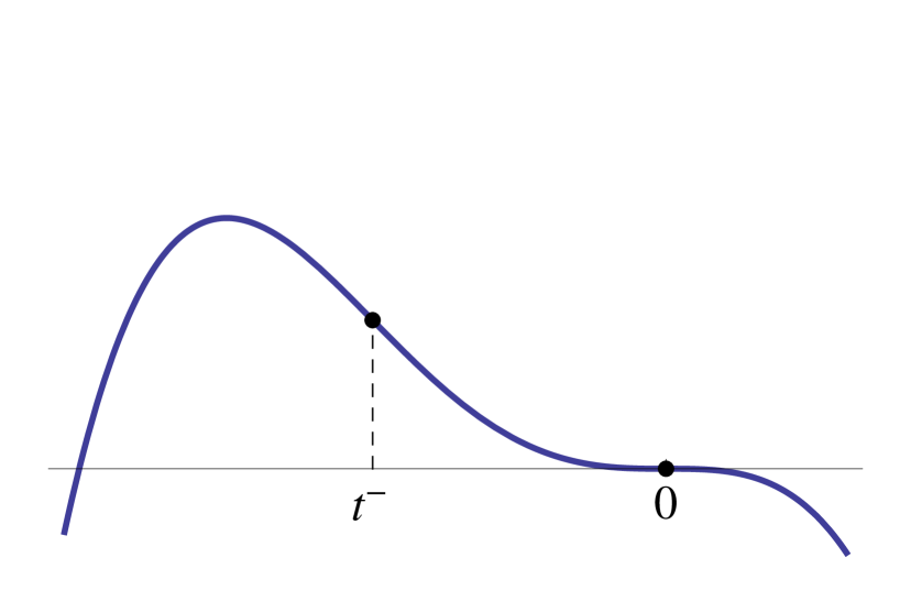
(a) $p_{2}=0$

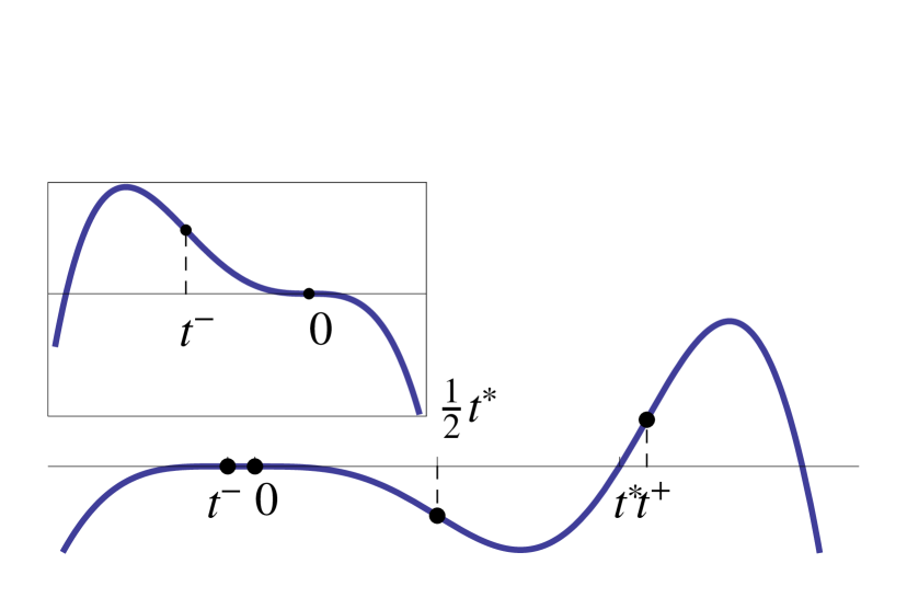
(b) $p_{2}<\alpha(p_{1})$

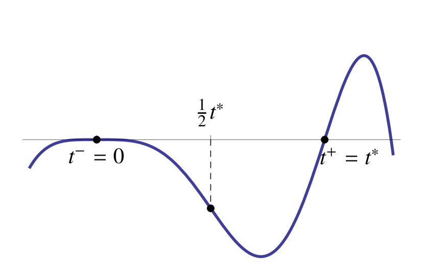
(c) $p_{2}=\alpha(p_{1})$

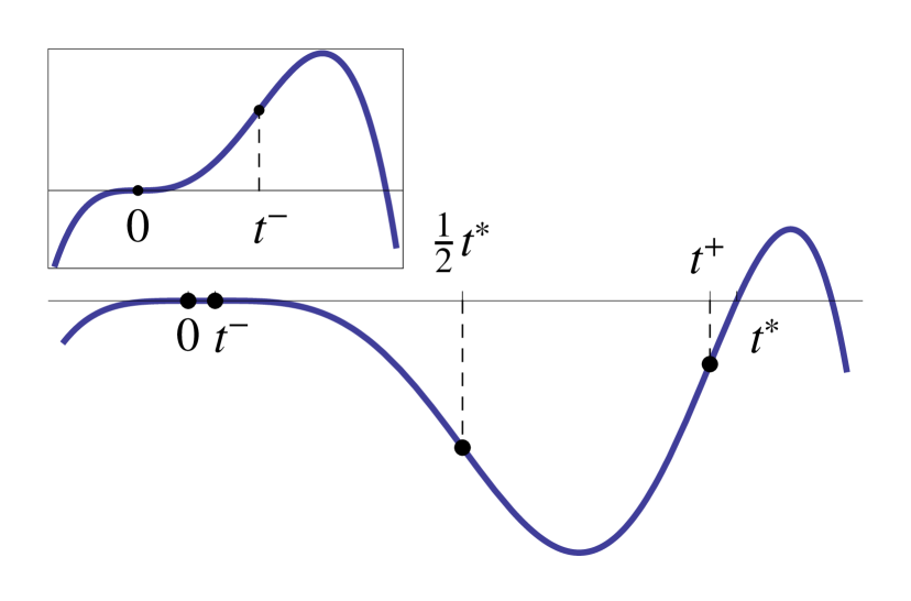
(d) $\alpha(p_{1})<p_{2}<\beta(p_{1})$

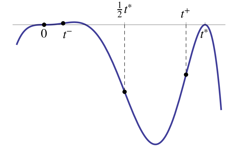
(e) $p_{2}=\beta(p_{1})$

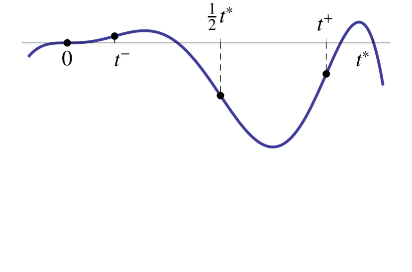
(f) $\beta(p_{1})<p_{2}<\gamma(p_{1})$

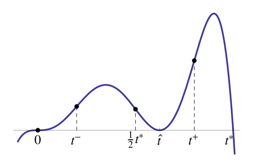
(g) $p_{2}=\gamma(p_{1})$

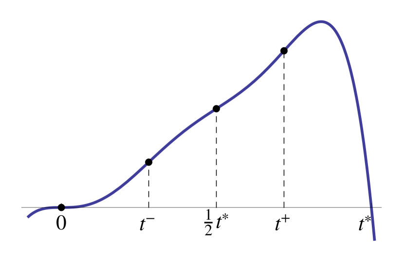
(h) $\gamma(p_{1})<p_{2}<\delta(p_{1})$

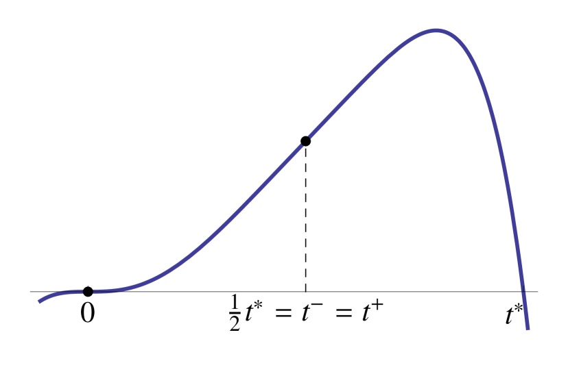
(i) $p_{2}=\delta(p_{1})$

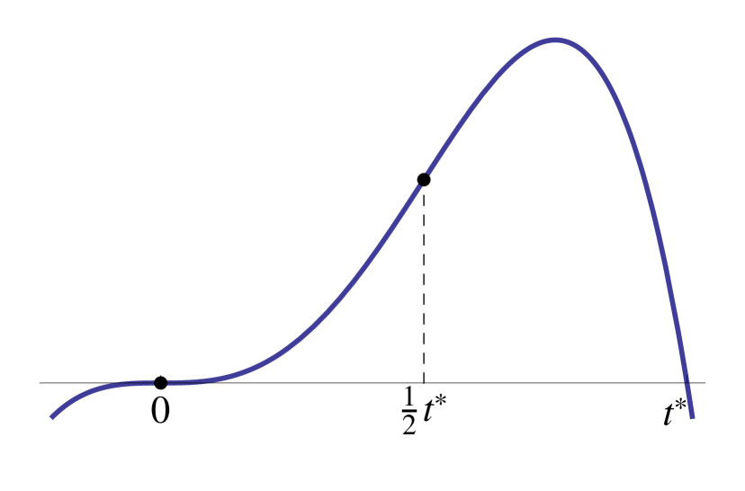
(j) $p_{2}>\delta(p_{1})$

Figure 3. Typical shapes of the functions $f_{p_{1},p_{2}}$ as $p_{2}$ increases. The axes in the panels are not the same scale. We marked the location $t^{\ast}$ of the maximum of $g_{p_{1},p_{2}}$ as well as the abscissas $0,t^{-},t^{+},t^{\ast}/2$ of the inflection points of $f_{p_{1},p_{2}}$. The value of $p_{1}$ is $0.7$.

Figure 2 suggests that $\beta(p_{1})$ exceeds $s_{t}(p_{1})$ if and only $p_{1}\geqslant u(t)$. This is indeed true and can be proved by analysing the sign of $h_{p_{1}}\left(s_{t}(p_{1})\right)$, where $h_{p_{1}}$ is the function defined in the proof of Proposition 3.4. The calculations are lengthy, however, and therefore omitted. We now complete the proof of the unimodality of $g_{p_{1},p_{2}}$ by analysing the sign of the function $f_{p_{1},p_{2}}$ on the interval $\left(0,t_{p_{1},p_{2}}^{\ast}\right)$.

Proposition 3.6.

There exists a function $\gamma:[0,p^{+}]\to[0,p^{-}]$ such that, for every $\langle p_{1},p_{2}\rangle\in\Delta$, the derivative of the function $g_{p_{1},p_{2}}$ is positive for $0<t<t_{p_{1},p_{2}}^{\ast}$ if and only if $p_{1}<p^{+}$ and $p_{2}>\gamma(p_{1})$.

Proof.

We will show that for every $p_{1}\in\left(0,p^{+}\right)$ there exists a positive number $\gamma(p_{1})\in\left[\beta(p_{1}),p^{-}\right)$ such that the function $f_{p_{1},p_{2}}(t)$ is positive on the interval $\left(0,t_{p_{1},p_{2}}^{\ast}\right)$ for all $p_{2}\in\left(\gamma(p_{1}),(p_{1},1-p_{1})^{-}\right)$.

Let $p_{1}<p^{+}$ be given. It follows from Proposition 3.4 that for $p_{2}<\beta(p_{1})$, the function $f_{p_{1},p_{2}}$ is not positive on $\left(0,t_{p_{1},p_{2}}^{\ast}\right)$ because it vanishes at $t=t_{p_{1},p_{2}}^{*}$ with positive derivative. It thus follows from the convexity properties of $f_{p_{1},p_{2}}$ (Lemma 3.2) that for $p_{2}<\beta(p_{1})$ the graph of $f_{p_{1},p_{2}}$ looks as in Fig. 3(d); in particular, it has a local minimum with abscissa in the interval $\left(t_{p_{1},p_{2}}^{\ast}/2,t_{p_{1},p_{2}}^{\ast}\right)$ and negative ordinate. As $p_{2}$ increases, first to $\beta(p_{1})$ and then beyond, the derivative of $f_{p_{1},p_{2}}$ at $t_{p_{1},p_{2}}^{*}$ changes sign, as depicted in Figs. 3(e) and 3(f). Increasing $p_{2}$ further, it follows from Lemma 3.1 and the intermediate value theorem that there must exist a smallest $\gamma(p_{1})$ in the interval $\left[\beta(p_{1}),(p_{1},1-p_{1})^{-}\right)$ such that $f_{p_{1},\gamma(p_{1})}$ has its local minimum at $\langle\hat{t}(p_{1}),0\rangle$ for some $\hat{t}(p_{1})\in\left(0,t_{p_{1},\gamma(p_{1})}^{\ast}\right)$. The graph of $f_{p_{1},\gamma(p_{1})}$ is depicted in Fig. 3(g).

In the following we will show that $f_{p_{1},p_{2}}(t)$ is positive on $\left(0,t_{p_{1},p_{2}}^{\ast}\right)$ for all $p_{2}\in\left(\gamma(p_{1}),p_{1}\right)$. This is equivalent to showing that, for all positive $t$, the value $f_{p_{1},p_{2}}(t)$ is positive for all points $\langle p_{1},p_{2}\rangle\in\Delta$ such that $p_{2}>\gamma(p_{1})$ and $t_{p_{1},p_{2}}^{\ast}>t$. If $p_{1}<p_{t}$ this is true because Lemma 3.5, i) shows that $f_{p_{1},p_{2}}$ is positive for all $p_{2}<p_{1}$. If $p_{t}\leqslant p_{1}<u(t)$, we observe that, by Eq. 3.9, the condition $t_{p_{1},p_{2}}^{\ast}>t$ is equivalent to the condition $p_{2}<s_{t}(p_{1})$ and that Lemma 3.5, ii) shows that $f_{p_{1},p_{2}}$ is positive for all $p_{2}\in\left(r_{t}(p_{1}),s_{t}(p_{1})\right)$. It thus remains to show that $r_{t}(p_{1})\leqslant\gamma(p_{1})$, which follows from the fact that $f_{p_{1},\gamma(p_{1})}(t)$ is positive. Finally, if $p_{1}\geqslant u(t)$, then $\gamma(p_{1})\geqslant\beta(p_{1})\geqslant s_{t}(p_{1})$, and there is thus nothing to prove. ∎

In the proof of Proposition 3.6, the boundary $\gamma$ has been defined only implicitly. The argument showed, however, that the set $C$, which for $p_{2}<(p_{1},1-p_{1})^{-}$ is characterised by the condition $p_{2}>\gamma(p_{1})$ and for other parts of $[0,1]^{2}$ by symmetry, is a non-empty subset of $B$. The inclusion $D\subset C$ follows from Theorem 1.3 and the fact that Proposition 3.6 is an if-and-only-if statement. The proof also showed that the triple $\langle p_{1},\gamma(p_{1}),\hat{t}(p_{1})\rangle$ satisfies the equations

$$f_{p_{1},\gamma(p_{1})}\left(\hat{t}(p_{1})\right)=f_{p_{1},\gamma(p_{1})}^{\prime}\left(\hat{t}(p_{1})\right)=0,\quad t_{p_{1},\gamma(p_{1})}^{\ast}/2<\gamma(p_{1})<t_{p_{1},\gamma(p_{1})}^{\ast},$$ (3.10)

and this can be used to solve for the boundary curve numerically. Alternatively, one might differentiate these equations implicitly and obtain a fairly complex system of differential equations for the functions $\gamma(\cdot)$, $\hat{t}(\cdot)$ which can be integrated numerically.

Finally, we can give a proof of our main result.

Proof of Theorem 1.2.

For $\langle p_{1},p_{2}\rangle\in\Delta$ parts i), ii) and iii) are proved in Propositions 3.3, 3.4 and 3.6, respectively. The boundary case $p_{2}=(p_{1},1-p_{1})^{-}$ is treated in Lemma 3.1. For other values of $p_{1}$, $p_{2}$ the claim follows by symmetry. ∎

References

Berend and Kontorovich [2013]
D. Berend and A. Kontorovich.
On the concentration of the missing mass.
Electron. Commun. Probab., 18(3):1–7,
2013.
Chen and Liu [1997]
S. X. Chen and J. S. Liu.
Statistical applications of the Poisson-binomial and conditional
Bernoulli distributions.
Statist. Sinica, 7(4):875–892, 1997.
Kearns and Saul [1998]
M. Kearns and L. Saul.
Large deviation methods for approximate probabilistic inference.
In Proceedings of the Fourteenth conference on Uncertainty in
artificial intelligence, pages 311–319. Morgan Kaufmann Publishers Inc.,
1998.