A multispecies birth–death–immigration process and its diffusion approximation

Abstract

We consider an extended birth-death-immigration process defined on a lattice formed by the integers of $d$ semiaxes joined at the origin. When the process reaches the origin, then it may jumps toward any semiaxis with the same rate. The dynamics on each ray evolves according to a one-dimensional linear birth-death process with immigration. We investigate the transient and asymptotic behavior of the process via its probability generating function. The stationary distribution, when existing, is a zero-modified negative binomial distribution. We also study a diffusive approximation of the process, which involves a diffusion process with linear drift and infinitesimal variance on each ray. It possesses a gamma-type transient density admitting a stationary limit.

As a byproduct of our study, we obtain a closed form of the number of permutations with a fixed number of components, and a new series form of the polylogarithm function expressed in terms of the Gauss hypergeometric function.

Keywords: Birth-death process; Diffusion process; Permutations with $k$ components; Polylogarithm function.

2010 Mathematics Subject Classification: 60J80; 60J85; 60J70

1 Introduction

We study a continuous-time stochastic process describing the dynamics of a population formed by a fixed number $d$ of non-interacting species competing for a single habitat. The problem of species competition is often approached in the literature by use of spatial models and competitive hierarchy. In some cases the number of species and the number of sites are fixed by assumption. See Buttel et al. [6], where specific attention is given to the number of species that can coexist on a finite number of sites. The models studied in Di Crescenzo et al. [12] take into account colonization, death and replacement, both in the presence and in absence of hierarchic rules for the species. In this paper we investigate a continuous-time stationary Markov chain ${\cal N}$, over a lattice formed by the integers of $d$ semiaxes joined at the origin, i.e. an extended star graph. This process is a suitable extension of a linear birth-death-immigration process (with constant immigration rates, and linear birth and death rates), and describes the dynamics of a population formed by $d$ non-interacting species into a given habitat. As soon as the habitat is occupied by an individual of a certain species (by effect of immigration) then the dynamics evolves according to a linear birth-death-immigration process until extinction. Next the habitat can be occupied again due to immigration of an individual of a possibly different species, and so on. In other terms, the local population is sustained primarily by reproduction of resident individuals, but may be subsidized by immigration of individuals of the same species. The rule of immigration, however, is seen mainly as allowing recolonization of the habitat after the extinction of the local population.

The linear birth-death process with immigration is often employed as a stochastic model for population processes in biology and ecology (see, for instance, Chao and Zheng [8], Crawford and Suchard [11], Kyriakidis [24], Ricciardi [29], Zheng et al. [33]). A birth-death-immigration process including the possibility of multiple immigrations has been discussed recently by Jakeman and Hopcraft [23]. We recall for instance the application of birth-death processes on graphs to evolutionary models of spatially structured populations. See Allen and Tarnita [2] for a comprehensive investigation on state-dependent birth-death population models with fixed population size and structure, and Broom and Rychtá$\check{\rm r}$ [4] for evolutionary dynamics of populations on graphs.

In this paper we first propose to investigate the distribution of the number of individuals of the local population, with special attention to the dependence of the stationary distribution on the number of species. We point out that the linear nature of birth and death rates allows us to obtain explicit closed-forms both for the transient and stationary dynamics of the process ${\cal N}$, rather than approximate or simulated results.

A further object of our investigation is the diffusive approximation of ${\cal N}$. The adopted procedure leads to a diffusion process with linear drift and infinitesimal variance, defined on the rays of a star graph. It is worth pointing out that we are able to study the transient behavior of the approximating diffusion process, via a gamma density with constant shape parameter and time-varying rate.

We recall that diffusion processes on graphs have been studied by several authors. See for instance Freidlin and Wentzell [17], that is one of the first contributions on this topic, and Weber [32] for occupation time functionals for diffusion processes and birth-death processes on graphs. An investigation involving a diffusion process on star graph has been performed in Papanicolaou et al. [28], where the authors obtain exit probabilities and certain other quantities involving exit and occupation times for a Brownian Motion on star graph. Other examples of diffusion processes on star graphs can be found in Mugnolo et al. [25].

This is the plan of the paper. In Section 2 we introduce the process ${\cal N}$ and its generator. In Section 3 we develop a generating function-based approach and obtain some useful integral equations. This allows us to get a formal expression for the transient probability that the process is located in the origin, i.e. the habitat is empty, the proof being provided in A. In Section 4 we perform the transient analysis of the process in two different cases. The adopted technique is based on the coupling of the homotopy perturbation method and an expansion in Taylor series. In Section 5 we use the Laplace transform to derive the asymptotic expression of the state probabilities (involving a zero-modified negative binomial distribution) and also of the mean and variance. Section 6 deals with the diffusive approximation of ${\cal N}$. We adopt a customary scaling that leads to a time-homogeneous diffusion process on the star graph, characterized by linear infinitesimal moments. A gamma-type stationary density is also obtained under suitable assumptions. In Section 7 we interpret our results in biological terms with special reference to the role of the number of species $d$. Finally, some concluding remarks are given in Section 8.

It is worth pointing out that, as a byproduct of our investigations, in Section 4 we provide some new results of wide interest in mathematics, i.e. a closed form of the number of permutations of $\{1,\ldots,n\}$ with $k$ components, also known as the number of permutations with $k-1$ global descents, and a new series form of the polylogarithm function expressed in terms of the Gauss hypergeometric function.

2 The stochastic model

Consider a habitat that may accommodate individuals of 1 out of $d$ population species, with $d\in\mathbb{N}^{+}$, and let $D=\{1,2,\ldots,d\}$. Assume that the evolution of individuals in the habitat is subject to births, deaths and immigrations, according to the following rules, where $h>0$ is sufficiently small:

(i)   If the habitat is empty at time $t$, then during the time interval $(t,t+h]$ either the habitat is occupied by an individual of species $j$, $(j\in D)$, with probability $\alpha h+o(h)$ (due to immigration), or it remains empty with probability $1-d\alpha h+o(h)$.

(ii)   If the habitat at time $t$ is occupied by $k$ individuals of species $j$, $(j\in D)$, then during the time interval $(t,t+h]$ either one individual dies with probability $\mu kh+o(h)$, or a new individual of the same species arrives with probability $(\alpha+\lambda k)h+o(h)$ (by the effect of immigration or birth), or the population size remains unchanged with probability $1-(\alpha+(\lambda+\mu)k)h+o(h)$.

Hence, note that when the habitat is empty each species may compete for the colonization of the habitat, whereas when a species occupies the habitat there is no interaction with other species.

Figure 1: Schematic representation of the state space $S$.

The dynamics is described by a continuous-time Markov chain ${\cal N}:=\{(N(t),J(t)),t\geq 0\}$, where $(N(t),J(t))=(0,0)$ if at time $t$ the habitat is empty, and $(N(t),J(t))=(k,j)$ if at time $t$ the habitat is occupied by $k$ individuals of the $j$-th species. The state space of ${\cal N}$ is the set $S=\{(0,0)\}\cup({\mathbb{N}}^{+}\times D)$, consisting of the integers of $d$ semiaxes $S_{1},S_{2},\ldots,S_{d}$ $(d\in\mathbb{N}^{+})$ with a common origin $(0,0)$ (see Figure 1). We denote the transition rates of ${\cal N}$ by

$$q({\bf u};{\bf v})=\lim_{h\rightarrow 0^{+}}\frac{1}{h}{\mathbb{P}}[(N(t+h),J(t+h))={\bf v}\,|\,(N(t),J(t))={\bf u}],\qquad{\bf u},{\bf v}\in S.$$

According to assumptions (i) and (ii), the generator $Q:=(q({\bf u};{\bf v}),{\bf u},{\bf v}\in S)$ of ${\cal N}$ satisfies

$$q(0,0;1,j)=\alpha,\qquad q(k,j;k+1,j)=\alpha+\lambda k,\qquad q(k,j;k-1,j)=\mu k,$$

$$q(k,j;r,j)=0\quad\hbox{if $|k-r|>1$},\qquad q(k,i;r,j)=0\quad\hbox{if $i\neq j$},$$ (1)

$$q(0,0;r,j)=q(r,j;0,0)=0\quad\hbox{if $r\neq 1$},$$

for all $k,r\in{\mathbb{N}}^{+}$ and $i,j\in D$, where $\alpha>0$, $\lambda>0$ and $\mu>0$ are constants denoting the immigration, birth and death rate per individual, respectively.

Noting that ${\cal N}$ is a skip-free process and that $(0,0)$ is a non-absorbing state, the above assumptions imply that ${\cal N}$ is nonexplosive (cf. Chen et al. [9]), and hence uniquely determined by $Q$.

If $d=1$ then ${\cal N}$ identifies with the linear birth-death process with immigration, that is well-known among population models (see Section 3.1 of Crawford and Suchard [11] and references therein). The purpose of our study is the extension of the birth-death-immigration process to the case of $d$ non-iteracting populations according to the assumptions indicated above.

3 Generating functions

We assume that the initial state of ${\cal N}$ is the origin, which for simplicity will be henceforth denoted as $0$ instead of $(0,0)$ . Hence, the transition probability of ${\cal N}$ is defined as

$$\begin{split}&p(k,j,\cdot)={\mathbb{P}}\{(N(\cdot),J(\cdot))=(k,j)\,|\,(N(0),J(0))=0\},\qquad k\in{\mathbb{N}}^{+},\;\;j\in D,\\ &p(0,\cdot)={\mathbb{P}}\{(N(\cdot),J(\cdot))=0\,|\,(N(0),J(0))=0\}.\end{split}$$ (2)

The initial condition is thus expressed as

$$\lim_{t\to 0^{+}}p(0,t)=1.$$ (3)

From (2) we have that

$$P(k,\cdot):=\sum_{j=1}^{d}p(k,j,\cdot),\qquad k\in{\mathbb{N}}^{+},$$ (4)

is the probability of occupancy of the $k$-th state of any semiaxis.

Consider the probability generating function

$$F(z,t)=p(0,t)+\sum_{k\geq 1}z^{k}P(k,t),\qquad z\in[0,1],\quad t\geq 0.$$ (5)

By virtue of (3), it satisfies the initial condition

$$F(z,0)=1,\qquad z\in[0,1].$$ (6)

Moreover, the following boundary conditions hold:

$$F(1,t)=1,\qquad t\geq 0,$$ (7)

$$F(0,t)=p(0,t),\qquad t\geq 0,$$ (8)

where $p(0,t)$ is the probability that the habitat is empty at time $t$.

Proposition 3.1

The generating function (5) satisfies the following differential equation for $z\in[0,1]$ and $t\geq 0$:

$${\partial\over\partial t}\!F(z,t)=-\alpha(d-1)(1-z)p(0,t)-\alpha(1-z)F(z,t)-(\lambda z-\mu)(1-z){\partial\over\partial z}\!F(z,t).$$ (9)

• Due to (1), for $k\in{\mathbb{N}}^{+}$ and $j\in D$, the following system of differential-difference equations holds for $t>0$:

  $${d\over dt}\;p(0,t)=\mu\sum_{j=1}^{d}p(1,j,t)-d\alpha\,p(0,t),$$ (10)

  $${d\over dt}\;p(k,j,t)=[\alpha+\lambda(k-1)]\,p(k-1,j,t)+\mu(k+1)\,p(k+1,j,t)-[\alpha+(\lambda+\mu)k]\,p(k,j,t).$$

  Hence, the probability generating function

  $$G_{j}(z,t):=\sum_{k\geq 1}z^{k}p(k,j,t),\qquad z\in[0,1],\quad t\geq 0,$$ (11)

  for $j\in D$ satisfies the following differential equation:

  $${\partial\over\partial t}G_{j}(z,t)=\mu p(1,j,t)+\alpha zp(0,t)-\alpha(1-z)G_{j}(z,t)-(\lambda z-\mu)(1-z){\partial\over\partial z}G_{j}(z,t).$$

  Hence, the proof of (9) follows recalling Eqs. (5) and (11). $\hfill\Box$

Here, and in the following, $f^{\prime}$ denotes the derivative of any function $f$.

Proposition 3.2

Eq. (9), with conditions (7) and (6), admits the following solution for $z\in[0,1]$ and $t\geq 0$:

$$F(z,t)=H(t)+(d-1)\int_{0}^{t}H^{\prime}(t-y)p(0,y){\rm d}y,$$ (12)

where

$$H(t)=h(t,z;\lambda,\mu):=\left\{\begin{array}[]{ll}\displaystyle{\frac{(\lambda-\mu)^{\frac{\alpha}{\lambda}}{\rm e}^{-\frac{\alpha}{\lambda}(\lambda-\mu)t}}{\left[\lambda(1-z)-(\mu-\lambda z)\,{\rm e}^{-(\lambda-\mu)t}\right]^{\frac{\alpha}{\lambda}}}},&\lambda\neq\mu,\\[14.22636pt] \displaystyle{\frac{1}{\left[1+\lambda t(1-z)\right]^{\frac{\alpha}{\lambda}}}},&\lambda=\mu.\end{array}\right.$$ (13)

• Let us adopt the method of characteristics. If $\lambda\neq\mu$, Eq. (9) can be rewritten as

  $$(\lambda z-\mu)(1-z){\partial F\over\partial z}+{\partial F\over\partial t}+\alpha(1-z)F+\alpha(d-1)(1-z)p(0,t)=0,$$ (14)

  which gives the following characteristic equations for the original system

  $${\displaystyle{dz\over ds}=(\lambda z-\mu)(1-z)},\qquad{\displaystyle{dt\over ds}=1},\qquad{\displaystyle{dF\over ds}=-\alpha(1-z)F-\alpha(d-1)(1-z)p(0,t)}.$$ (15)

  From Eq. (15), along the characteristic curves

  $$z=1-\frac{(\lambda-\mu)(1-\tau)}{\lambda(1-\tau)-(\mu-\lambda\tau){\rm e}^{(\lambda-\mu)s}},\qquad t=s,\qquad\tau\in{\mathbb{R}},$$

  the partial differential equation (14) and conditions (6) and (7) yield

  $$\frac{{\rm d}F}{{\rm d}s}+\alpha\left[\frac{(\lambda-\mu)(1-\tau)}{\lambda(1-\tau)-(\mu-\lambda\tau){\rm e}^{(\lambda-\mu)s}}\right]F+\alpha(d-1)\displaystyle\left[\frac{(\lambda-\mu)(1-\tau)}{\lambda(1-\tau)-(\mu-\lambda\tau){\rm e}^{(\lambda-\mu)s}}\right]p(0,s)=0,$$

  with $F(0)=1$. Hence, Eqs. (12) and (13) follow after some calculations. If $\lambda=\mu$, the proof is similar. $\hfill\Box$

Hereafter we show that $p(0,t)$ satisfies a linear Volterra integral equation of the 2nd kind.

Corollary 3.1

The following renewal equation holds, for $t>0$,

$$p(0,t)=1-G(t)-(d-1)\int_{0}^{t}G^{\prime}(t-y)p(0,y){\rm d}y,$$ (16)

where

$$G(t)=1-h(t,0;\lambda,\mu),$$ (17)

with $h(t,z;\lambda,\mu)$ defined in (13).

• Eqs. (16) and (17) follow from Eqs. (12) and (13), for $z=0$ and recalling condition (8). $\hfill\Box$

We remark that $G(t)$, given in (17), is a proper distribution function when $\lambda\geq\mu$.

Hereafter we consider the distribution function

$$F_{Y}^{(j)}(t):={\mathbb{P}}(Y_{1}+Y_{2}+\cdots+Y_{j}\leq t),$$ (18)

where $Y_{1},Y_{2},\ldots,Y_{j}$ is a sequence of i.i.d. random variables. In the following theorem we give a formal representation of $p(0,t)$ in terms of (18) when $Y_{i}$’s are nonnegative and have a specific distribution.

Theorem 3.1

For $t\geq 0$ we have

$$p(0,t)=\left\{\begin{array}[]{ll}\displaystyle{1-{d}\sum_{j=1}^{+\infty}(1-d)^{j-1}F_{Y}^{(j)}(t)},&\quad\lambda\geq\mu,\\[8.5359pt] \displaystyle{1-{d}\sum_{j=1}^{+\infty}(1-d)^{j-1}\left[1-\left(\frac{\mu-\lambda}{\mu}\right)^{\frac{\alpha}{\lambda}}\right]^{j}F_{Y}^{(j)}(t)},&\quad\lambda<\mu,\\[11.38092pt] \end{array}\right.$$ (19)

where

$$F_{Y}^{(1)}(t)=\left\{\begin{array}[]{ll}\displaystyle{1-\left(\frac{\lambda-\mu}{\lambda{\rm e}^{(\lambda-\mu)t}-\mu}\right)^{\frac{\alpha}{\lambda}}},&\quad\lambda>\mu,\\[8.5359pt] \displaystyle{1-\frac{1}{(1+\lambda t)^{\frac{\alpha}{\lambda}}}},&\quad\lambda=\mu,\\[11.38092pt] \displaystyle{\frac{1}{1-\left(1-\frac{\lambda}{\mu}\right)^{\frac{\alpha}{\lambda}}}\,\left[1-\left(\frac{\mu-\lambda}{\mu-\lambda{\rm e}^{-(\mu-\lambda)t}}\right)^{\frac{\alpha}{\lambda}}\right]},&\quad\lambda<\mu.\\[11.38092pt] \end{array}\right.$$ (20)

The proof of Theorem 20 is given in A.

Remark 3.1

The right-hand-side of Eq. (20), in each of the three cases, identifies with the distribution function of suitable transformations of a random variable, say $Z$, having Pareto type II (Lomax) distribution with shape and scale parameters $\tilde{\alpha}$ and $\tilde{\lambda}$, respectively. Namely,
$\bullet$  if $\lambda>\mu$, then $F_{Y}^{(1)}(t)$ is the distribution function of $\log{(Z+1)}/(\lambda-\mu)$, with $\tilde{\alpha}=\alpha/\lambda$ and $\tilde{\lambda}=(\lambda-\mu)/\lambda$,
$\bullet$  if $\lambda=\mu$, then $F_{Y}^{(1)}(t)$ is the distribution function of $Z$ for $\tilde{\alpha}=\alpha/\lambda$ and $\tilde{\lambda}=1/\lambda$,
$\bullet$  if $\lambda<\mu$, then $F_{Y}^{(1)}(t)$ is the distribution function of $-\log{(1-Z)}/(\mu-\lambda)$, assuming that $Z$ has support $(0,1)$ and parameters $\tilde{\alpha}=\alpha/\lambda$ and $\tilde{\lambda}=(\mu-\lambda)/\lambda$.

4 Transient analysis

In this section, for $t$ ranging over specified intervals of $\mathbb{R}$, we obtain explicit expressions for the generating function $F(z,t)$ and for the transient probability $p(0,t)$ that the habitat is empty. We also study the cumulative probability $P(k,t)$, i.e. the probability that the habitat is occupied by $k$ individuals (irrespective of their species) at time $t$. We consider 2 cases:
1. Immigration, birth and death rates are equal ($\alpha=\lambda=\mu$).
2. Immigration and birth rates are equal, the death rate is different ($\alpha=\lambda$ and $\mu\neq\lambda$).

4.1 Transient analysis for $\alpha=\lambda=\mu$

Aiming to obtain an expression for $p(0,t)$ when $\alpha=\lambda=\mu$, let us denote by $t_{n,k}$ the number of permutations of $\{1,\ldots,n\}$, $n\geq 1$, with $k\geq 1$ components (see, for instance, Comtet [10], p. $262$ and [27]). Alternatively, $t_{n,k}$ is the number of permutations of $\{1,\ldots,n\}$ with $k-1$ global descents. Permutations with one component, i.e. $t_{n,1}$, are known as indecomposable permutations (we recall that a permutation is called indecomposable if its one-line notation cannot be split into two parts such that every number in the first part is smaller than every number in the second part). Noting that $t_{n,k}=0$ if $n<k$, an implicit recursion formula for $t_{n,k}$ is given by (see Propositions 2.4 and 2.7 of [21])

$$t_{n,k}=\left\{\begin{array}[]{ll}n!-\displaystyle{\sum_{j=1}^{n-1}(n-j)!\cdot t_{j,1}},&k=1,\\[17.07182pt] \displaystyle{\sum_{j=1}^{n-k+1}t_{j,1}\cdot t_{n-j,k-1}},&2\leq k\leq n.\end{array}\right.$$ (21)

Proposition 4.1

Let $\alpha=\lambda=\mu$. If $0<t<1/\lambda$ the integral equation (16) admits the following solution:

$$p(0,t)=1+\sum_{n=1}^{+\infty}\frac{(-\lambda t)^{n}}{n!}\sum_{j=1}^{n}t_{n,j}\,d^{j}.$$ (22)

• The proof is based on the coupling of the homotopy perturbation method and the expansion of the involved functions as Taylor series (see Biazar and Eslami [3]). From (16), for $\alpha=\lambda=\mu$, we can construct the following homotopy

  $$H(p,q)=p(0,t)-\frac{1}{(1+\lambda t)}+\lambda(d-1)q\int_{0}^{t}\frac{p(0,y)}{[1+\lambda(t-y)]^{2}}{\rm d}y=0,$$ (23)

  with the embedding parameter $q$. By assuming that $p(0,t)=\sum_{n=0}^{+\infty}q_{n}(t)q^{n}$ and substituting functions $\frac{1}{(1+\lambda t)}$ and $\frac{1}{[1+\lambda(t-y)]^{2}}$ by their Taylor series forms, in agreement with Eq. (23) we define

  $$\widetilde{H}(p,q)=\sum_{n=0}^{+\infty}q_{n}(t)q^{n}-\sum_{n=0}^{+\infty}(-\lambda t)^{n}q^{n}+\lambda(d-1)\sum_{n=0}^{+\infty}q^{n+1}\int_{0}^{t}\alpha_{n}(y,t){\rm d}y=0,$$ (24)

  for $0<t<1/\lambda$, with

  $$\alpha_{n}(y,t)=\sum_{k=0}^{n}q_{k}(y)(n-k+1)[-\lambda(t-y)]^{n-k}.$$ (25)

  Hence, equating the coefficients of the terms with identical powers of $q$, we find that function $q_{n}(x)$ is solution of the following recursive equation:

  $$q_{n}(x)=(-\lambda x)^{n}-\lambda(d-1)\int_{0}^{x}\alpha_{n-1}(y,x){\rm d}y,\qquad n\in\mathbb{N}^{+},$$ (26)

  with $q_{0}(x)=1$. By direct calculations, from Eq. (26) one immediately gets

  $$q_{1}(x)=-d\lambda x.$$

  Hereafter we make use of the strong induction principle to show that

  $$q_{n}(x)=\frac{(-\lambda x)^{n}}{n!}\sum_{j=1}^{n}t_{n,j}\,d^{j},\qquad n\in\mathbb{N}^{+}.$$ (27)

  Being $t_{k,k}=1$ for all $k\geq 1$ (see [10], p. $262$), Eq. (27) holds for $n=1$. Assuming that (27) holds for all $k=1,2,\ldots,n$ we now prove that it holds true for $k=n+1$. From Eq. (25), due to the induction hypothesis, we have

  $$\int_{0}^{x}\alpha_{n}(y,x){\rm d}y=x\frac{(-\lambda x)^{n}}{(n+1)!}\sum_{j=1}^{n}(n+1-j)!\sum_{r=1}^{j}t_{j,r}\,d^{r}+x(-\lambda x)^{n},\qquad n\in\mathbb{N}^{+}.$$

  Hence, recalling Eq. (26) and using $t_{k,k}=1$ $\forall k\geq 1$, we obtain

  $$q_{n+1}(x)=\frac{(-\lambda x)^{n+1}}{({n+1})!}\left\{d\,({n+1})!+(d-1)\sum_{j=1}^{n}(n+1-j)!\sum_{r=1}^{j}t_{j,r}\,d^{r}\right\}$$ (28)

  $$\hskip 34.14322pt=\frac{(-\lambda x)^{n+1}}{(n+1)!}\left\{d\left[(n+1)!-\sum_{j=1}^{n}(n+1-j)!\,t_{j,1}\right]+d^{n+1}\right.$$

  $$\hskip 36.98866pt\left.+\sum_{s=2}^{n}d^{s}\left[(n-s+2)!+\sum_{j=s}^{n}(n+1-j)!(t_{j,s-1}-t_{j,s})\right]\right\}.$$

  Recalling Eq. (21), we note that

  $$\sum_{j=s}^{n}(n+1-j)!\cdot t_{j,s}=\sum_{r=s-1}^{n-1}t_{r,s-1}\sum_{j=r+1}^{n}(n+1-j)!\cdot t_{j-r,1}.$$

  Hence, repeated applications of Eq. (21) yield

  $$(n-s+2)!t_{s-1,s-1}+\sum_{j=s}^{n}(n+1-j)!(t_{j,s-1}-t_{j,s})$$

  $$=(n-s+2)!+\sum_{r=s}^{n-1}t_{r,s-1}\Bigg{[}(n+1-r)!-\sum_{j=r+1}^{n}(n+1-j)!t_{j-r,1}\Bigg{]}+\,t_{n,s-1}-\sum_{j=s}^{n}(n+1-j)!t_{j-s+1,1}$$

  $$=(n-s+2)!+\sum_{r=s}^{n}t_{r,s-1}\cdot t_{n+1-r,1}-\sum_{j=s}^{n}(n+1-j)!t_{j-s+1,1}$$

  $$=t_{n-s+2,1}+\sum_{r=s}^{n}t_{r,s-1}\cdot t_{n+1-r,1}=t_{n+1,s}.$$ (29)

  From Eqs. (28) and (29) we thus obtain Eq. (27). Finally, by taking $q=1$ in assumption $p(0,t)=\sum_{n=0}^{+\infty}q_{n}(t)q^{n}$ we get Eq. (22). $\hfill\Box$

Proposition 4.2

If $\alpha=\lambda=\mu$, then for $0<t<1/\lambda$ we have

$$F(z,t)=\frac{1}{1+\lambda t(1-z)}-\frac{\lambda t(d-1)(1-z)}{1+\lambda t(1-z)}\left[1+\sum_{n=1}^{+\infty}\frac{(-\lambda t)^{n}}{n!}\sum_{j=1}^{n}t_{n,j}\,d^{j}\right]-\frac{(d-1)(1-z)}{[1+\lambda t(1-z)]^{2}}$$

$$\hskip 11.38092pt\times\sum_{n=1}^{+\infty}n\frac{(-\lambda t)^{n+1}}{(n+1)!}\,{}_{2}F_{1}\left(1,n+1;n+2;1-\frac{1}{1+\lambda t(1-z)}\right)\sum_{j=1}^{n}t_{n,j}\,d^{j},$$ (30)

where

$${}_{2}F_{1}(a,b;c;z)=\sum_{n=0}^{+\infty}\frac{(a)_{n}(b)_{n}}{(c)_{n}}\,\frac{z^{n}}{n!}$$ (31)

is the Gauss hypergeometric function. (Here, and in the remainder of the paper, $(d)_{n}=d(d+1)(d+2)\cdots(d+n-1)$, $n\geq 1$, denotes the Pochhammer symbol, with $(d)_{0}=1$ for $d\neq 0$.)

• From Eqs. (12), (13) and (22), we obtain

  $$F(z,t)=\frac{1}{1+\lambda t(1-z)}-\frac{\lambda t(d-1)(1-z)}{1+\lambda t(1-z)}-(d-1)\sum_{n=1}^{+\infty}\frac{(-\lambda t)^{n}}{n!}\sum_{j=1}^{n}t_{n,j}\,d^{j}$$

  $$\hskip 11.38092pt+\frac{(d-1)}{1+\lambda t(1-z)}\sum_{n=1}^{+\infty}\frac{(-\lambda t)^{n}}{n!}\,{}_{2}F_{1}\left(1,n;n+1;1-\frac{1}{1+\lambda t(1-z)}\right)\sum_{j=1}^{n}t_{n,j}\,d^{j}.$$

  Hence, making use of Eqs. $15.2.25$ and $15.1.8$ of [1], after some calculations we come to Eq. (30). $\hfill\Box$

We now obtain probability (4) under the assumptions of Propositions 4.1 and 4.2.

Proposition 4.3

If $\alpha=\lambda=\mu$, for $0<t<1/\lambda$ we have

$$P(k,t)=\frac{(\lambda t)^{k}}{(\lambda t+1)^{k+1}}\left\{d+(d-1)\sum_{n=1}^{+\infty}\frac{(-\lambda t)^{n}}{n!}\sum_{j=1}^{n}t_{n,j}\,d^{j}\right.$$

$$\hskip 17.07182pt\left.\times\sum_{r=0}^{+\infty}\frac{(n)_{r}}{(n+1)_{r}}\left(1-\frac{1}{1+\lambda t}\right)^{r}\,{}_{2}F_{1}\left(-r,-k;1;-\frac{1}{\lambda t}\right)\right\}.$$ (32)

• From Eq. (30), and recalling (22) and (31), we have

  $$F(z,t)=\frac{1}{1+\lambda t(1-z)}-(d-1)p(0,t)\frac{\lambda t(1-z)}{1+\lambda t(1-z)}$$

  $$-\frac{(d-1)(1-z)}{[1+\lambda t(1-z)]^{2}}\sum_{k=0}^{+\infty}\left[1-\frac{1}{1+\lambda t(1-z)}\right]^{k}\sum_{n=1}^{+\infty}\frac{(-\lambda t)^{n+1}}{(n-1)!(n+k+1)}\sum_{j=1}^{n}t_{n,j}\,d^{j}$$

  $$=p(0,t)+\sum_{m=0}^{+\infty}z^{m}\frac{(\lambda t)^{m}}{(\lambda t+1)^{m+1}}-p(0,t)\left[\frac{1+d\lambda t}{1+\lambda t}-(d-1)\sum_{m=1}^{+\infty}z^{m}\frac{(\lambda t)^{m}}{(\lambda t+1)^{m+1}}\right]$$

  $$-(d-1)\sum_{m=0}^{+\infty}z^{m}\frac{(\lambda t)^{m}}{(\lambda t+1)^{m+2}}\sum_{n=1}^{+\infty}\frac{(-\lambda t)^{n+1}}{(n-1)!}\sum_{j=1}^{n}t_{n,j}\,d^{j}\sum_{k=0}^{+\infty}\frac{\left(\frac{\lambda t}{\lambda t+1}\right)^{k}}{n+k+1}\,{}_{2}F_{1}\left(-k-1,-m;1;-\frac{1}{\lambda t}\right).$$

  Hence, since $p(0,t)$ satisfies the integral equation (16), it results

  $$F(z,t)=p(0,t)+\sum_{m=1}^{+\infty}z^{m}\frac{(\lambda t)^{m}}{(\lambda t+1)^{m+1}}+p(0,t)(d-1)\sum_{m=1}^{+\infty}z^{m}\frac{(\lambda t)^{m}}{(\lambda t+1)^{m+1}}$$

  $$\hskip 5.69046pt+(d-1)\sum_{m=1}^{+\infty}z^{m}\frac{(\lambda t)^{m+1}}{(\lambda t+1)^{m+2}}\sum_{n=1}^{+\infty}\frac{(-\lambda t)^{n}}{(n-1)!}\sum_{j=1}^{n}t_{n,j}\,d^{j}$$

  $$\hskip 5.69046pt\times\sum_{k=0}^{+\infty}\frac{(n+1)_{k}}{(n+2)_{k}\,(n+1)}\left(\frac{\lambda t}{\lambda t+1}\right)^{k}\,{}_{2}F_{1}\left(-k-1,-m;1;-\frac{1}{\lambda t}\right).$$

  Finally, recalling Eq. (5) and equating the coefficients of the terms with identical powers of $z$ we obtain Eq. (32). $\hfill\Box$

 

Figure 2: Plots of $p(0,t)$ and $P(1,t)$ for $\lambda=0.5$, $\mu=0.5$ and $\alpha=0.5$, for $d=1,2,3,4,10$, from top to bottom for $p(0,t)$, and from bottom to top for $P(1,t)$.

In Figure 2 we show some plots obtained by means of the expressions given in Proposition 4.1 and Proposition 4.3.

4.2 Transient analysis for $\alpha=\lambda$ and $\mu\neq\lambda$

In order to investigate the case $\alpha=\lambda$ and $\mu\neq\lambda$, we set for brevity

$$Q_{j,m}\equiv Q_{j,m}\left(\frac{\mu}{\lambda}\right):=\sum_{\begin{subarray}{c}s_{1},\ldots,s_{j}\geq 2\\ s_{1}+\cdots+s_{j}=m\end{subarray}}A_{s_{1}}\left(\frac{\mu}{\lambda}\right)\times\cdots\times A_{s_{j}}\left(\frac{\mu}{\lambda}\right),$$ (33)

where $A_{n}(t)$ are the Eulerian Polynomials (see, for instance, Foata [16] or Hirzebruch [22]).

Proposition 4.4

If $\alpha=\lambda$ and $\mu\neq\lambda$, then for $0<t<\log(\mu/\lambda)/(\mu-\lambda)$ the integral equation (16) admits the following solution

$$p(0,t)=1-d\left\{1-\frac{\mu-\lambda}{\mu-\lambda{\rm e}^{-(\mu-\lambda)t}}-\frac{1}{d-1}\left[{\rm e}^{-\lambda t(d-1)}-1+\lambda t(d-1)\right]\right.$$

$$\hskip 2.84544pt\left.-\sum_{n=3}^{\infty}\frac{(-\lambda t)^{n}}{n!}\sum_{k=1}^{n-2}(d-1)^{k}\sum_{j=1}^{n-k-1}{k+1\choose j}Q_{j,j+n-k-1}\right\}.$$ (34)

• The proof proceeds similarly as that of Proposition 4.1. Recalling Eq. (17), for $0<t<\log(\mu/\lambda)/(\mu-\lambda)$ we have

  $$1-G(t)=\frac{\frac{\mu}{\lambda}-1}{\frac{\mu}{\lambda}-{\rm e}^{-\lambda t\left(\frac{\mu}{\lambda}-1\right)}}=\sum_{n=0}^{\infty}A_{n}\left(\frac{\mu}{\lambda}\right)\frac{(-\lambda t)^{n}}{n!}.$$ (35)

  The radius of convergence of the power series in Eq. (35) has been determined finding the location (in the complex plane) of the singularity nearest to the origin. We can construct the following homotopy

  $$H(p,q)=\sum_{n=0}^{+\infty}q_{n}(t)q^{n}-\sum_{n=0}^{+\infty}A_{n}\left(\frac{\mu}{\lambda}\right)\frac{(-\lambda t)^{n}}{n!}q^{n}$$

  $$+\lambda(d-1)\sum_{n=0}^{+\infty}q^{n+1}\sum_{j=0}^{n}A_{j+1}\left(\frac{\mu}{\lambda}\right)\int_{0}^{t}\frac{(-\lambda y)^{j}}{j!}q_{n-j}(t-y){\rm d}y=0,$$ (36)

  where $q$ is the embedding parameter and we have set $p(0,t)=\sum_{n=0}^{+\infty}q_{n}(t)q^{n}$. We thus find that $q_{n}(t)$ satisfies the following recursive equation:

  $$q_{n}(t)=A_{n}\left(\frac{\mu}{\lambda}\right)\frac{(-\lambda t)^{n}}{n!}-\lambda(d-1)\sum_{j=0}^{n-1}A_{j+1}\left(\frac{\mu}{\lambda}\right)\int_{0}^{t}\frac{(-\lambda y)^{j}}{j!}q_{n-1-j}(t-y){\rm d}y.$$ (37)

  By straightforward calculations, from Eq. (37) one immediately gets

  $$q_{0}(t)=1,\qquad q_{1}(t)=-d\lambda t,\qquad q_{2}(t)=\lambda d(\mu+\lambda d)\frac{t^{2}}{2}.$$ (38)

  Let us now make use of the strong induction principle to show that, for $n\geq 3$,

  $$q_{n}(t)=d\,\frac{(-\lambda t)^{n}}{n!}\bigg{\{}\sum_{k=1}^{n-2}(d-1)^{k}\sum_{j=1}^{n-k-1}{k+1\choose j}Q_{j,j+n-k-1}+A_{n}\left(\frac{\mu}{\lambda}\right)+(d-1)^{n-1}\bigg{\}}.$$ (39)

  By direct calculations, it follows from (37) and (38) that

  $$q_{3}(t)=-\lambda d[\lambda^{2}d^{2}+2\lambda\mu(d+1)+\mu^{2}]\frac{t^{3}}{3!},$$

  which is equal to Eq. (39) for $n=3$, being $A_{3}(z)=1+4z+z^{2}$. Let us consider $n\geq 3$ and assume that Eq. (39) holds for all $r=2,\ldots,n-1$. We shall prove that identity (39) holds also for $r=n$. From Eq. (37), recalling (38) we have

  $$q_{n}(t)=dA_{n}\left(\frac{\mu}{\lambda}\right)\frac{(-\lambda t)^{n}}{n!}+d(d-1)A_{n-1}\left(\frac{\mu}{\lambda}\right)\frac{(-\lambda t)^{n}}{n!}$$

  $$-\lambda(d-1)\sum_{r=2}^{n-1}A_{n-r}\left(\frac{\mu}{\lambda}\right)\int_{0}^{t}\frac{(-\lambda y)^{n-1-r}}{(n-1-r)!}q_{r}(t-y){\rm d}y.$$

  Hence, due to the induction hypothesis (39), we obtain

  $$q_{n}(t)=d\frac{(-\lambda t)^{n}}{n!}\bigg{\{}A_{n}\left(\frac{\mu}{\lambda}\right)+(d-1)A_{n-1}\left(\frac{\mu}{\lambda}\right)$$ (40)

  $$+(d-1)\sum_{r=2}^{n-1}A_{n-r}\left(\frac{\mu}{\lambda}\right)A_{r}\left(\frac{\mu}{\lambda}\right)+\sum_{r=2}^{n-1}(d-1)^{r}A_{n-r}\left(\frac{\mu}{\lambda}\right)$$

  $$+\sum_{r=3}^{n-1}A_{n-r}\left(\frac{\mu}{\lambda}\right)\sum_{k=1}^{r-2}(d-1)^{k+1}\sum_{j=1}^{r-k-1}{k+1\choose j}Q_{j,j+r-k-1}\bigg{\}}$$

  $$=d\frac{(-\lambda t)^{n}}{n!}\left\{A_{n}\left(\frac{\mu}{\lambda}\right)+\sum_{r=1}^{n-1}(d-1)^{r}A_{n-r}\left(\frac{\mu}{\lambda}\right)\right.$$

  $$\left.+\sum_{h=1}^{n-2}(d-1)^{h}\sum_{j=1}^{n-1-h}{h\choose j}\sum_{r=1}^{n-j-h}A_{r}\left(\frac{\mu}{\lambda}\right)Q_{j,n+j-h-r}\right\}.$$

  Noting that

  $$\sum_{r=1}^{n-j-h}A_{r}\left(\frac{\mu}{\lambda}\right)Q_{j,n+j-h-r}=Q_{j,n+j-h-1}+Q_{{j+1},n+j-h},$$

  from Eq. (40) we obtain

  $$q_{n}(t)=d\frac{(-\lambda t)^{n}}{n!}\left\{A_{n}\left(\frac{\mu}{\lambda}\right)+\sum_{r=1}^{n-1}(d-1)^{n-r}A_{r}\left(\frac{\mu}{\lambda}\right)\right.$$

  $$+\sum_{r=2}^{n-1}(d-1)^{n-r}\sum_{k=1}^{r-1}{n-r\choose k}Q_{k,r+k-1}\left.+\sum_{r=2}^{n-1}(d-1)^{n-r}\sum_{k=2}^{r}{n-r\choose k-1}Q_{k,r+k-1}\right\}$$

  $$=d\frac{(-\lambda t)^{n}}{n!}\left\{A_{n}\left(\frac{\mu}{\lambda}\right)+\sum_{r=1}^{n-1}(d-1)^{n-r}A_{r}\left(\frac{\mu}{\lambda}\right)\right.$$

  $$+\sum_{r=2}^{n-1}(d-1)^{n-r}(n-r)A_{r}\left(\frac{\mu}{\lambda}\right)\left.+\sum_{r=2}^{n-1}(d-1)^{n-r}\sum_{k=2}^{r-1}{n-r+1\choose k}Q_{k,r+k-1}\right\}$$

  $$=d\frac{(-\lambda t)^{n}}{n!}\left\{A_{n}\left(\frac{\mu}{\lambda}\right)+(d-1)^{n-1}+\sum_{r=2}^{n-1}(d-1)^{n-r}\sum_{k=1}^{r-1}{n-r+1\choose k}Q_{k,r+k-1}\right\},$$

  which gives Eq. (39). By setting $q=1$ in assumption $p(0,t)=\sum_{n=0}^{+\infty}q_{n}(t)q^{n}$, and recalling (39), we finally obtain Eq. (34). $\hfill\Box$

Remark 4.1

If $d=1$ the expressions for $p(0,t)$ given in Theorem 20, Proposition 4.1 and Proposition 4.4 are in agreement with the well-known results for the linear birth-death process with immigration (see, for instance, Section 2.3 of Nucho [26]).

Hereafter we derive an explicit expression for $t_{n,k}$ in terms of multinomial coefficients, for $n\geq 2$ and $1\leq k\leq n$. It is worth pointing out that a closed form expression for such numbers does not appear to have been obtained before.

Corollary 4.1

The following equalities hold for $n\geq 2$:

$$t_{n,1}=n!+(-1)^{n-1}+\sum_{k=1}^{n-2}(-1)^{k}\sum_{j=1}^{n-k-1}{k+1\choose j}(n-k-1+j)!\sum_{\begin{subarray}{c}s_{1},\ldots,s_{j}\geq 2\\ s_{1}+\cdots+s_{j}=n-k-1+j\end{subarray}}\frac{1}{{n-k-1+j\choose s_{1},\ldots,s_{j}}};$$

$$t_{n,k}={n-1\choose k-1}(-1)^{n-k}+\sum_{r=k-1}^{n-2}{r\choose k-1}(-1)^{r-k+1}\sum_{j=1}^{n-r-1}{r+1\choose j}$$

$$\hskip 2.84544pt\times(n-r-1+j)!\sum_{\begin{subarray}{c}s_{1},\ldots,s_{j}\geq 2\\ s_{1}+\cdots+s_{j}=n-r-1+j\end{subarray}}\frac{1}{{n-r-1+j\choose s_{1},\ldots,s_{j}}},\hskip 71.13188pt2\leq k\leq n-1;$$

$$t_{n_{,}n}=1.$$

• The proof follows from Propositions 4.1 and 4.4, by letting $\mu\to\lambda$ and noting that $A_{j}(1)=j!$. $\hfill\Box$

In the following proposition we obtain the probability generating function when $\mu\neq\lambda$ and $\alpha=\lambda$. In the sequel we shall denote by

$$\theta_{n}\equiv\theta_{n}(\lambda,\mu,d):=\sum_{i=1}^{n-2}(d-1)^{i}\sum_{j=1}^{n-i-1}{i+1\choose j}Q_{j,j+n-i-1}+A_{n}\left(\frac{\mu}{\lambda}\right)+(d-1)^{n-1},$$ (41)

where $Q_{j,m}$ is defined in Eq. (33).

Proposition 4.5

If $\alpha=\lambda$ and $\mu\neq\lambda$, for $t<\log(\mu/\lambda)/(\mu-\lambda)$, it is

$$F(z,t)=1-d+\frac{d(\mu-\lambda)}{\mu-\lambda z-\lambda(1-z){\rm e}^{-(\mu-\lambda)t}}-\frac{d(d-1)(\mu-\lambda)^{2}}{\mu-\lambda z}$$

$$\times\Big{[}-\lambda g_{1}(z)+\sum_{n=2}^{+\infty}\frac{(-\lambda)^{n}}{n!}g_{n}(z)\theta_{n}\Big{]}$$ (42)

where

$$g_{k}(z)=\left\{\begin{array}[]{l}\frac{1}{(\lambda-\mu)^{k+1}}\left\{\lambda(1-z)(\lambda-\mu)^{k-1}t^{k}+k!\left[{\rm Li}_{k}\left(\frac{\lambda(1-z){\rm e}^{-(\mu-\lambda)t}}{\mu-\lambda z}\right)\right.\right.\\ \left.\left.\qquad\qquad-{\rm Li}_{k}\left(\frac{\lambda(1-z)}{\mu-\lambda z}\right)\right]-\sum_{r=1}^{k-1}\frac{k!}{r!}[(\lambda-\mu)t]^{r}{\rm Li}_{k-r}\left(\frac{\lambda(1-z)}{\mu-\lambda z}\right)\right\}\\ \hskip 227.62204pt\hbox{if }\mu>\lambda,\\[11.38092pt] \frac{1}{(\mu-\lambda)^{k+1}}\left\{(\mu-\lambda z)(\mu-\lambda)^{k-1}t^{k}+k!\left[{\rm Li}_{k}\left(\frac{(\mu-\lambda z){\rm e}^{-(\lambda-\mu)t}}{\lambda(1-z)}\right)\right.\right.\\ \qquad\qquad\left.\left.-{\rm Li}_{k}\left(\frac{\mu-\lambda z}{\lambda(1-z)}\right)\right]-\sum_{r=1}^{k-1}\frac{k!}{r!}\,[(\mu-\lambda)t]^{r}\,{\rm Li}_{k-r}\left(\frac{\mu-\lambda z}{\lambda(1-z)}\right)\right\}\\ \hskip 227.62204pt\hbox{if }\mu<\lambda,\end{array}\right.$$

and where

$${\rm Li}_{k}(z)=\sum_{j=1}^{+\infty}\frac{z^{j}}{j^{k}}$$ (43)

is the polylogarithm function.

• It immediately follows from Eqs. (12) and (13), recalling Eq. (34). $\hfill\Box$

We conclude this section by evaluating the probability (4).

Proposition 4.6

Let $k\in\mathbb{N}^{+}$. If $\alpha=\lambda$, for $t<\log(\mu/\lambda)/(\mu-\lambda)$, we have
$\bullet$ for $\mu>\lambda$

$$P(k,t)=\frac{\lambda^{k}}{\mu^{k+1}}\left\{d(\mu-\lambda)\mu^{k+1}\frac{[1-{\rm e}^{-(\mu-\lambda)t}]^{k}}{[\mu-\lambda{\rm e}^{-(\mu-\lambda)t}]^{k+1}}-d(d-1)(\lambda-\mu)\right.$$ (44)

$$\hskip 17.07182pt\left.\times\left[-\lambda t+\sum_{n=2}^{+\infty}\frac{(-\lambda t)^{n}}{n!}\theta_{n}\right]-\lambda d(d-1)\sum_{l=1}^{+\infty}\frac{(1-{\rm e}^{-l(\mu-\lambda)t})}{l}{}_{2}F_{1}^{*}\right.$$

$$\hskip 17.07182pt\left.+d(d-1)\sum_{n=2}^{+\infty}\frac{(-\lambda)^{n}}{(\lambda-\mu)^{n-1}}\theta_{n}\sum_{r=1}^{n-1}\frac{[(\lambda-\mu)t]^{r}}{r!}\sum_{l=1}^{+\infty}\frac{1}{l^{n-r}}{}_{2}F_{1}^{*}\right.$$

$$\hskip 17.07182pt\left.+d(d-1)\sum_{n=2}^{+\infty}\frac{(-\lambda)^{n}}{(\lambda-\mu)^{n-1}}\theta_{n}\sum_{l=1}^{+\infty}\frac{1-{\rm e}^{-l(\mu-\lambda)t}}{l^{n}}{}_{2}F_{1}^{*}\right\},$$

where ${}_{2}F_{1}^{*}={}_{2}F_{1}\left(-l,k+1;1;1-\frac{\lambda}{\mu}\right)$;
$\bullet$ for $\mu<\lambda$

$$P(k,t)=d(\lambda-\mu){\rm e}^{-(\lambda-\mu)t}\frac{[\lambda\,(1-{\rm e}^{-(\lambda-\mu)t})]^{k}}{[\lambda-\mu{\rm e}^{-(\lambda-\mu)t}]^{k+1}}-d(d-1)\frac{\lambda}{\mu}\,{\rm Li}_{k+1}\left(\frac{\mu}{\lambda}\right)$$ (45)

$$\hskip 25.6073pt+d(d-1)\sum_{s=1}^{+\infty}\frac{{\rm e}^{-s(\lambda-\mu)t}}{s}{}_{2}F_{1}^{**}$$

$$\hskip 25.6073pt+\frac{d(d-1)}{\lambda}\sum_{n=2}^{+\infty}\frac{(-\lambda)^{n}}{(\mu-\lambda)^{n-1}}\theta_{n}\sum_{s=1}^{+\infty}\frac{(1-{\rm e}^{-s(\lambda-\mu)t})}{s^{n}}{}_{2}F_{1}^{**}$$

$$\hskip 25.6073pt+\frac{d(d-1)}{\lambda}\sum_{n=2}^{+\infty}\frac{(-\lambda)^{n}}{(\mu-\lambda)^{n-1}}\theta_{n}\sum_{r=1}^{n-1}\frac{[(\mu-\lambda)t]^{r}}{r!}\sum_{s=1}^{+\infty}\frac{1}{s^{n-r}}{}_{2}F_{1}^{**},$$

where $\theta_{n}$ is defined in Eq. (41), and ${}_{2}F_{1}^{**}={}_{2}F_{1}\left(1-s,k+1;1;1-\frac{\mu}{\lambda}\right)$.

• The proof follows from Eqs. (5) and (42), recalling that $p(0,t)$ satisfies the integral equation (16), noting that (see Eq. (65.1.3) of [20], for instance)

  $$\sum_{k=0}^{+\infty}\frac{(d)_{k}}{k!}y^{k}{}_{2}F_{1}\left(-k,b;c;x\right)=(1-y)^{-d}{}_{2}F_{1}\left(d,b;c;\frac{xy}{y-1}\right),$$

  and making use of (43). $\hfill\Box$

 

Figure 3: Plots of $p(0,t)$ and $P(1,t)$ for $\lambda=0.1$, $\mu=0.5$ and $\alpha=0.1$, for $d=1,2,3,4,10$, from top to bottom for $p(0,t)$, and from bottom to top for $P(1,t)$.

 

Figure 4: Plots of $p(0,t)$ and $P(1,t)$ for $\lambda=0.5$, $\mu=0.1$ and $\alpha=0.5$, for $d=1,2,3,4$, from top to bottom for $p(0,t)$, and from bottom to top for $P(1,t)$.

In Figures 3 and 4 we show some plots of $p(0,t)$ and $P(1,t)$ obtained by evaluating the expressions given in Proposition 4.4 and Proposition 4.6.

Let us now provide a simple relation between the polylogarithm function and a series of Gauss hypergeometric functions, which does not appear to have been given before. This result immediately follows from Proposition 4.6.

Corollary 4.2

For all $k\in\mathbb{N}^{+}$ and $x\in(0,1)$ we have

$${\rm Li}_{k+1}(x)=x\sum_{s=1}^{+\infty}\frac{1}{s}\left[{}_{2}F_{1}\left(1-s,k+1;1;1-x\right)\right].$$ (46)

• The proof of (46) follows from (45), by taking into account that $P(k,0)=0$. $\hfill\Box$

A classical problem in population birth-death models is the extinction, i.e. the first passage through the zero state (see, e.g. Van Doorn and Zeifman [31]). However, in our model this problem reduces to a well-known one-dimensional case.

We finally conclude the analysis of $\cal N$ by discussing some asymptotic results.

5 Asymptotic results

According to the one-dimensional case, ${\cal N}$ admits a stationary distribution if and only if $\lambda<\mu$. In the following proposition we obtain explicitly the expression of the stationary probabilities

$$\rho(0):=\lim_{t\rightarrow+\infty}p(0,t),\qquad\rho(k):=\lim_{t\rightarrow+\infty}P(k,t),\quad k\in\mathbb{N}^{+}.$$

Proposition 5.1

If $\lambda<\mu$, then

$$\rho(0)=\frac{1}{d}\,\displaystyle{\frac{\left(1-\frac{\lambda}{\mu}\right)^{\frac{\alpha}{\lambda}}}{1-\left(1-\frac{1}{d}\right)\left(1-\frac{\lambda}{\mu}\right)^{\frac{\alpha}{\lambda}}}},$$ (47)

$$\rho(k)=\displaystyle{\frac{\left(1-\frac{\lambda}{\mu}\right)^{\frac{\alpha}{\lambda}}}{1-\left(1-\frac{1}{d}\right)\left(1-\frac{\lambda}{\mu}\right)^{\frac{\alpha}{\lambda}}}\,\frac{(\frac{\alpha}{\lambda})_{k}}{k!}\,\left(\frac{\lambda}{\mu}\right)^{k}},\qquad k\in\mathbb{N}^{+}.$$ (48)

If $\lambda\geq\mu$, then $\rho(k)=0$ for $k\in\mathbb{N}_{0}$.

• Eq. (47) follows from Theorem 20. Denoting by

  $${\cal L}_{s}[f(t)]=\int_{0}^{+\infty}{\rm e}^{-st}f(t){\rm d}t,\qquad s\geq 0,$$ (49)

  the Laplace transform of an arbitrary function $f(t)$, from Proposition 13 we have

  $${\cal L}_{s}[F(z,t)]={\cal L}_{s}[H(t)]+(d-1)(s\,{\cal L}_{s}[H(t)]-1)\,{\cal L}_{s}[p(0,t)].$$ (50)

  Note that, due to Eq. (10) of Section 2.1.3, p. 59, of Erdélyi et al. [15],

  $${\cal L}_{s}[H(t)]=\left\{\begin{array}[]{ll}\displaystyle{\frac{\lambda(\lambda-\mu)^{\frac{\alpha}{\lambda}}{}_{2}F_{1}(\frac{\alpha}{\lambda},\frac{\alpha}{\lambda}+\frac{s}{\lambda-\mu};\frac{\alpha}{\lambda}+\frac{s}{\lambda-\mu}+1;\frac{\mu-\lambda z}{\lambda(1-z)})}{\left[\lambda(1-z)\right]^{\frac{\alpha}{\lambda}}\left[\lambda s+\alpha(\lambda-\mu)\right]}},&\lambda>\mu,\\[11.38092pt] \displaystyle{\frac{(\mu-\lambda)^{{\frac{\alpha}{\lambda}}-1}}{(\mu-\lambda z)^{\frac{\alpha}{\lambda}}}\frac{\mu-\lambda}{s}{}_{2}F_{1}\left(\frac{\alpha}{\lambda},\frac{s}{\mu-\lambda};\frac{s}{\mu-\lambda}+1;\frac{\lambda(1-z)}{\mu-\lambda z}\right)},&\lambda<\mu,\\[11.38092pt] \displaystyle{\frac{{\rm e}^{\frac{s}{\lambda(1-z)}}E\left(\frac{\alpha}{\lambda},\frac{s}{\lambda(1-z)}\right)}{\lambda(1-z)}},&\lambda=\mu,\end{array}\right.$$

  where

  $$E(\nu,z):=\int_{1}^{+\infty}\frac{{\rm e}^{-zt}}{t^{\nu}}{\rm d}t,\quad\nu\in{\mathbb{R}},\quad z>0,$$ (51)

  denotes the generalized exponential integral function and ${}_{2}F_{1}$ is defined in (31). Hence, recalling the Tauberian theorem, and making use of Eqs. (47) and (50), we have

  $$\lim_{t\to+\infty}F(z,t)=\left\{\begin{array}[]{ll}0,&\lambda\geq\mu,\\[5.69046pt] \displaystyle{\frac{(\mu-\lambda)^{\frac{\alpha}{\lambda}}}{(\mu-\lambda z)^{\frac{\alpha}{\lambda}}}\left[1+\frac{(d-1)\left(\frac{\mu-\lambda}{\mu}\right)^{\frac{\alpha}{\lambda}}}{d-(d-1)\left(\frac{\mu-\lambda}{\mu}\right)^{\frac{\alpha}{\lambda}}}\right]}\displaystyle-\frac{(d-1)\left(\frac{\mu-\lambda}{\mu}\right)^{\frac{\alpha}{\lambda}}}{d-(d-1)\left(\frac{\mu-\lambda}{\mu}\right)^{\frac{\alpha}{\lambda}}},&\lambda<\mu.\end{array}\right.$$ (52)

  If $\lambda<\mu$, making use of

  $$\frac{(\mu-\lambda)^{\frac{\alpha}{\lambda}}}{(\mu-\lambda z)^{\frac{\alpha}{\lambda}}}=\sum_{k=0}^{+\infty}\frac{(\frac{\alpha}{\lambda})_{k}}{k!}\left(1-\frac{\lambda}{\mu}\right)^{\frac{\alpha}{\lambda}}\left(\frac{\lambda}{\mu}\right)^{k}z^{k}$$

  and recalling Eq. (5), after some calculations we obtain (48) from Eqs. (47) and (52). $\hfill\Box$

Remark 5.1

From the stationary probabilities (47) and (48) we have that, for $\lambda<\mu$, the following identity holds for $k\in\mathbb{N}_{0}$:

$$\rho(k)=\vartheta_{d}\,\pi(k)+(1-\vartheta_{d})\,{\bf 1}_{\{k=0\}},\qquad\left(\vartheta_{d}=\left[{1-\left(1-\frac{1}{d}\right)\left(1-\frac{\lambda}{\mu}\right)^{\frac{\alpha}{\lambda}}}\right]^{-1}\right),$$ (53)

where $\pi(k)$ is the negative binomial distribution given by

$$\pi(k)=\left(1-\frac{\lambda}{\mu}\right)^{\frac{\alpha}{\lambda}}\frac{(\frac{\alpha}{\lambda})_{k}}{k!}\,\left(\frac{\lambda}{\mu}\right)^{k},\qquad k\in\mathbb{N}_{0}.$$

We note that if $d=1$ then $\vartheta_{d}=1$, and thus $\rho(k)=\pi(k)$, $\forall k\in\mathbb{N}_{0}$. Moreover, $\vartheta_{d}$ is increasing in $d\geq 1$ and tends to a constant when $d\to+\infty$.

Denoting by $N$ the discrete random variable having distribution $\{\rho(k);\;k\in\mathbb{N}_{0}\}$, after some calculations we obtain the following mean and variance, for $\lambda<\mu$:

$$E[N]=\vartheta_{d}\,\displaystyle\frac{\alpha}{\mu-\lambda},\qquad Var[N]=\vartheta_{d}^{2}\,\displaystyle\frac{\alpha\mu}{(\mu-\lambda)^{2}}\left[1-\left(1-\frac{1}{d}\right)\left(\frac{\alpha}{\mu}+1\right)\left(1-\frac{\lambda}{\mu}\right)^{\frac{\alpha}{\lambda}}\right].$$ (54)

6 The diffusion approximation

In this section we construct a diffusion approximation for the process $\cal N$. We adopt a scaling procedure that is customary in queueing theory contexts (see, for instance, Di Crescenzo et al. [13]). First of all, we perform a different parameterization of the model studied in Section 2 by setting

$$\alpha=\tilde{\gamma}\,{\tilde{\mu}\over\epsilon},\qquad\lambda={\tilde{\mu}\over\epsilon}+\tilde{\beta},\qquad\mu={\tilde{\mu}\over\epsilon},$$ (55)

with $\tilde{\gamma}>0$, $\tilde{\mu}>0$, $\tilde{\beta}\in\mathbb{R}$ and $\epsilon>0$. Note that $\epsilon$ is a positive constant that can be viewed as a measure of the size of $\tilde{\mu}$. It plays a crucial role in the approximating procedure indicated below, where $\epsilon\to 0^{+}$.

For all $t>0$, consider the scaling $N^{*}_{\epsilon}(t)=N(t)\,\epsilon$, so that ${\cal N}^{*}_{\epsilon}:=\{(N^{*}_{\epsilon}(t),J(t));\;t\geq 0\}$ is a continuous-time stochastic process having state space $S_{\epsilon}^{*}=\{0\}\cup\left(\mathbb{N}^{+}_{\epsilon}\times D\right)$, where $\mathbb{N}^{+}_{\epsilon}=\{\epsilon,2\epsilon,3\epsilon,\ldots\}$. The transient probabilities, for $t\geq 0$, $k\in\mathbb{N}_{0}$, $j\in D$, are given by

$$p^{*}_{\epsilon}(0,t)\!\! := \!\!{\mathbb{P}}\left\{(N^{*}_{\epsilon}(t),J(t))=0\right\},$$

$$p^{*}_{\epsilon}(k,j,t)\!\! := \!\!{\mathbb{P}}\left\{(N^{*}_{\epsilon}(t),J(t))=(k\epsilon,j)\right\}={\mathbb{P}}\left\{k\epsilon\leq N^{*}_{\epsilon}(t)<(k+1)\epsilon,J(t)=j\right\}.$$

In the limit as $\epsilon\to 0^{+}$, the scaled process ${\cal N}^{*}_{\epsilon}$ is shown to converge weakly to a diffusion process ${\cal X}:=\{(X(t),J(t));\;t\geq 0\}$, whose state space is the star graph $S_{\cal X}:=\{0\}\cup\left(\mathbb{R}^{+}\times D\right)$. For $x\in\mathbb{R}^{+}$, $t\geq 0$ and $j\in D$, let ${\mathbb{P}}\{x\leq X(t)<x+\epsilon,J(t)=j\}=f(x,j,t)\epsilon+o(\epsilon)$, so that $f(x,j,t)$ denotes the density of the process in state $x$ on the ray $S_{j}$.

Proposition 6.1

For $x\in\mathbb{R}^{+}$, $t>0$ and $j\in D$, the following differential equation holds:

$${\partial\over\partial t}\;f(x,j,t)=-{\partial\over\partial x}\;\Bigl{\{}(\tilde{\beta}\,x+\tilde{\gamma}\,\tilde{\mu})\,f(x,j,t)\Bigr{\}}+{1\over 2}\,{\partial^{2}\over\partial x^{2}}\Bigl{\{}2\,\tilde{\mu}\,x\,f(x,j,t)\Bigr{\}},$$ (56)

with boundary condition

$$\sum_{j=1}^{d}\lim_{x\to 0^{+}}\Bigl{\{}(\tilde{\beta}\,x+\tilde{\gamma}\,\tilde{\mu})\,f(x,j,t)-{1\over 2}\,{\partial\over\partial x}\bigl{[}2\,\tilde{\mu}\,x\,f(x,j,t)\bigr{]}\Bigr{\}}=0.$$ (57)

• Since $p^{*}_{\epsilon}(k,j,t)=p(k,j,t)$, due to (55) and in analogy with system (10), for $j\in D$ and $t>0$ we have

  $$p^{*}_{\epsilon}(0,t+\Delta t)=\sum_{j=1}^{d}p^{*}_{\epsilon}(1,j,t)\,{\tilde{\mu}\over\epsilon}\Delta t+p^{*}_{\epsilon}(0,t)\,\left(1-d\tilde{\gamma}\,{\tilde{\mu}\over\epsilon}\Delta t\right)+o(\Delta t),$$ (58)

  $$p^{*}_{\epsilon}(k,j,t+\Delta t)=p^{*}_{\epsilon}(k-1,j,t)\,\left[\tilde{\gamma}\,{\tilde{\mu}\over\epsilon}+\left({\tilde{\mu}\over\epsilon}+\tilde{\beta}\right)(k-1)\right]\Delta t+p^{*}_{\epsilon}(k+1,j,t)\,{\tilde{\mu}\over\epsilon}\,(k+1)\Delta t$$

  $$\hskip 39.83368pt+p^{*}_{\epsilon}(k,j,t)\,\left\{1-\left[\tilde{\gamma}\,{\tilde{\mu}\over\epsilon}+\left(2{\tilde{\mu}\over\epsilon}+\tilde{\beta}\right)k\right]\Delta t\right\}+o(\Delta t),\qquad k\in\mathbb{N}^{+}.$$ (59)

  Let $p^{*}_{\epsilon}(k,j,t)\simeq f(k\epsilon,j,t)\,\epsilon$ for $\epsilon$ close to 0. Hence, for $x=k\epsilon$, from Eq. (59) we have

  $$f(x,j,t+\Delta t)\!\! = \!\!f(x-\epsilon,j,t)\,\left[\tilde{\gamma}\,\tilde{\mu}+\left({\tilde{\mu}\over\epsilon}+\tilde{\beta}\right)(x-\epsilon)\right]{\Delta t\over\epsilon}+f(x+\epsilon,j,t)\,\tilde{\mu}\,(x+\epsilon){\Delta t\over\epsilon}$$

  $$+ \!\!f(x,j,t)\,\left\{1-\left[\tilde{\gamma}\,\tilde{\mu}+\left(2{\tilde{\mu}\over\epsilon}+\tilde{\beta}\right)x\right]{\Delta t\over\epsilon}\right\}+o(\Delta t).$$

  Expanding $f$ as Taylor series, by setting $\Delta t=A\,\epsilon^{2}$, with $A>0$, and passing to the limit as $\epsilon\to 0^{+}$, we obtain Eq. (56). Similarly, Eq. (58) yields

  $$f(0,t+\Delta t)=\sum_{j=1}^{d}f(\epsilon,j,t)\,\tilde{\mu}\,{\Delta t\over\epsilon}+f(0,t)\left(1-d\tilde{\gamma}\tilde{\mu}\,{\Delta t\over\epsilon}\right)+o(\Delta t),$$

  so that (57) holds. $\hfill\Box$

From the above procedure, the following approximation holds: ${\mathbb{P}}\{N(t)<k\}\simeq{\mathbb{P}}\{X(t)<k\epsilon\}$, this being expected to improve as $\epsilon\to 0^{+}$ and $k\to+\infty$.

Let us now introduce the density

$$h(x,t):=\sum_{j=1}^{d}f(x,j,t),\qquad x\in\mathbb{R}^{+},\quad t\geq 0.$$ (60)

Proposition 6.2

For $x\in\mathbb{R}^{+}$ and $t>0$, the transition density (60) satisfies the following differential equation:

$${\partial\over\partial t}\;h(x,t)=-{\partial\over\partial x}\;\Bigl{\{}(\tilde{\beta}\,x+\tilde{\gamma}\,\tilde{\mu})\,h(x,t)\Bigr{\}}+{1\over 2}\,{\partial^{2}\over\partial x^{2}}\Bigl{\{}2\,\tilde{\mu}\,x\,h(x,t)\Bigr{\}},$$ (61)

with boundary condition

$$\lim_{x\to 0^{+}}\Bigl{\{}(\tilde{\beta}\,x+\tilde{\gamma}\,\tilde{\mu})\,h(x,t)-{1\over 2}\,{\partial\over\partial x}\bigl{[}2\,\tilde{\mu}\,x\,h(x,t)\bigr{]}\Bigr{\}}=0$$ (62)

and Dirac-delta initial condition

$$\lim_{t\to 0^{+}}h(x,t)=\delta(x).$$ (63)

• The proof of Eqs. (61) and (62) follows immediately from Proposition 6.1, and recalling position (60). The condition (63) can be obtained from (3). $\hfill\Box$

Note that Eq. $(\ref{eq:equdiffsomma})$ is the Fokker-Planck equation for a temporally homogeneous diffusion process on $\mathbb{R}^{+}$ with linear drift and linear infinitesimal variance, while Eq. $(\ref{eq:equdiffbound})$ expresses a zero-flux condition in the state $x=0$. We remark that various results on such kind of diffusion process have been given in Buonocore et al. [5], Giorno et al. [18], and Sacerdote [30], for instance.

Hereafter we show that $h(x,t)$ is a gamma density with shape parameter $\tilde{\gamma}$ and rate $\psi(t)$.

Proposition 6.3

Let $\psi(t)=(\tilde{\beta}/\tilde{\mu})({\rm e}^{\tilde{\beta}t}-1)^{-1}$, $t>0$. The density (60) is given by

$$h(x,t)=\frac{[\psi(t)]^{\tilde{\gamma}}}{\Gamma(\tilde{\gamma})}\,x^{\tilde{\gamma}-1}\,{\rm e}^{-x\psi(t)},\qquad x\in\mathbb{R}^{+},\quad t>0.$$ (64)

• The transformation (see Capocelli and Ricciardi [7])

  $$x^{\prime}=x\,{\rm e}^{-\tilde{\beta}t},\qquad t^{\prime}=\frac{\tilde{\mu}}{\tilde{\beta}}\left(1-{\rm e}^{-\tilde{\beta}t}\right),\qquad h(x,t)={\rm e}^{-\tilde{\beta}t}\,h^{\prime}(x^{\prime},t^{\prime}),$$

  changes equation (61) and condition (62) respectively into a Fokker-Planck equation for the time-homogeneous diffusion process on $\mathbb{R}^{+}$ having drift $\tilde{\gamma}$ and infinitesimal variance $2x^{\prime}$, with a zero-flux condition on the boundary $x^{\prime}=0$. Initial condition (63) becomes $\displaystyle\lim_{t^{\prime}\to 0^{+}}h^{\prime}(x^{\prime},t^{\prime})=\delta(x^{\prime})$. The proof thus proceeds similarly as Proposition 4.1 of Di Crescenzo and Nobile [14] assuming a zero initial state. $\hfill\Box$

 

Figure 5: Density (64) for $t=0.5,1,2,3,4$ (from top to bottom near the origin), for $\tilde{\mu}=1$, $\tilde{\gamma}=1.5$ and (a) $\tilde{\beta}=-1$, (b) $\tilde{\beta}=1$.

In Figure 5 we show some plots of density $h(x,t)$.

From Eq. (64) we immediately obtain that a gamma-type stationary density exists when $\tilde{\beta}<0$.

Corollary 6.1

If $\tilde{\beta}<0$, then

$$\overline{h}(x):=\lim_{t\rightarrow+\infty}h(x,t)=\frac{1}{\Gamma(\tilde{\gamma})}\Bigg{(}\frac{|\tilde{\beta}|}{\tilde{\mu}}\Bigg{)}^{\!\tilde{\gamma}}x^{\tilde{\gamma}-1}\,\exp\Bigg{(}-x\,\frac{|\tilde{\beta}|}{\tilde{\mu}}\Bigg{)},\qquad x\in\mathbb{R}^{+}.$$ (65)

It is worthwhile to note that the validity of the diffusion approximation discussed in the present section is ascertained by comparing the stationary laws of the involved processes. Indeed, performing the substitutions (55) in Eqs. (47) and (48) it is not hard to prove that

$$\lim_{\varepsilon\to 0^{+}}\frac{1}{\varepsilon}\rho(k)\Big{|}_{k=x/\varepsilon}=\overline{h}(x),$$

with $\overline{h}(x)$ given in (65). Similarly, from (54) we obtain

$$\lim_{\varepsilon\to 0^{+}}E[\varepsilon N]=\tilde{\gamma}\,\frac{\tilde{\mu}}{|\tilde{\beta}|}=E[X],\qquad\lim_{\varepsilon\to 0^{+}}Var[\varepsilon N]=\tilde{\gamma}\,\left(\frac{\tilde{\mu}}{|\tilde{\beta}|}\right)^{2}=Var[X],$$

where $X$ denotes the random variable having density (65).

7 Discussion

In order to discuss some results obtained in the previous sections, we first consider $p(0,t)$, i.e. the probability of extinction of the population at finite times $t$. This finite-time probability deserves large interest since in many situations researchers cannot observe in a reliable manner the population dynamics for very long times. Figures 2, 3 and 4 confirm that $p(0,t)$ decreases linearly in $\alpha$ and $d$ when $t$ is close to $0$. Indeed, from (10) and (3) we have ${d\over dt}\;p(0,t)|_{t=0}=-d\alpha$, and clearly ${d\over dt}\;P(1,t)|_{t=0}=d\alpha$. Hence, in this multispecies model the number of species and the immigration rate play a similar role to increase the survival probability for short times.

Let us now focus on the stationary distribution obtained in Proposition 5.1 for $\lambda<\mu$. From Eq. (48) we note that $\rho(k)\geq\rho(k+1)$ when $k\geq\max\{1,(\alpha-\mu)/(\mu-\lambda)\}$. Hence, if the immigration rate is smaller than the death rate then the sequence $\{\rho(k),\;k\in\mathbb{N}^{+}\}$ is decreasing whatever $d$ is. Instead, condition $\rho(0)\geq\rho(1)$ holds when $d\alpha\leq\mu$. This implies the following results:

(a)  when $\alpha\leq\mu$ then $\rho(0)\geq\rho(1)\geq\rho(2)\geq\ldots$ if $1\leq d\leq\mu/\alpha$, and $\rho(0)\leq\rho(1)\geq\rho(2)\geq\ldots$ otherwise;

(b)  when $\alpha>\mu$ then $\rho(0)\leq\rho(1)\leq\ldots\leq\rho(k^{*})\geq\rho(k^{*}+1)\geq\ldots$ for $k^{*}=\lceil(\alpha-\mu)/(\mu-\lambda)\rceil$.

In other terms, if $\alpha\leq\mu$ the ratio between the death rate and the immigration rate is a critical value for the number of species, since the stationary probability of extinction is larger than the stationary probability of any other state $k\in\mathbb{N}^{+}$, if $1\leq d\leq\mu/\alpha$. However, even if $d\geq\mu/\alpha\geq 1$ the stationary distribution attains its maximum for $k=1$. Instead, a large immigration rate (i.e., $\alpha>\mu$) yields a larger mode $k^{*}$ for the stationary probability distribution. From Eq. (54) we have that the mode $k^{*}$ is very close to the stationary expected number of individuals when $d$ is large. This is confirmed, for instance, by the contour plots of $k^{*}=\lceil(\alpha-\mu)/(\mu-\lambda)\rceil$ and $E[N]$ (for $d=10$), shown in Figure 6 when $0<\lambda/\mu<1<\alpha/\mu<100$.

 

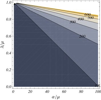
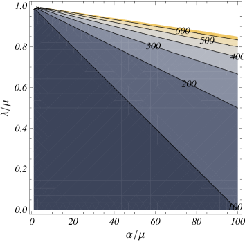
Figure 6: Contour plots of $k^{*}=\lceil(\alpha-\mu)/(\mu-\lambda)\rceil$ (left) and $E[N]$ for $d=10$ (right).

In order to emphasize the dependence on $d$ of the stationary distribution obtained in Proposition 5.1, we note that $\rho(0)$ is decreasing in $d\in\mathbb{N}^{+}$, whereas $\rho(k)$ is increasing in $d\in\mathbb{N}^{+}$ for $k\in\mathbb{N}^{+}$. Hence, if the number of species increases then the stationary probability of extinction decreases.

From Eq. (54) we have that if $d$ grows then $E[N]$ increases, going to a finite limit when $d\to+\infty$. In particular, this illustrates that when $\lambda<\mu$ the expected number of individuals does not grow indefinitely in the steady state. Moreover, we can adopt the coefficient of variation as an adimensional normalized measure of dispersion. For $\lambda<\mu$, we have that $CV[N]=\sqrt{Var[N]}/E[N]$ is decreasing in $d\in\mathbb{N}^{+}$ and tends to a finite limit:

$$\lim_{d\to+\infty}CV[N]=\sqrt{\frac{\mu}{\alpha}-\left(1+\frac{\mu}{\alpha}\right)\left(1-\frac{\lambda}{\mu}\right)^{\alpha/\lambda}}.$$

Another dispersion measure of interest in biological modeling is entropy. We recall that the (Shannon) entropy of a random variable $N$ with probability distribution $\{\rho(k);k\in\mathbb{N}_{0}\}$ is defined as

$$H[N]=-\sum_{k=0}^{+\infty}\rho(k)\ln[\rho(k)].$$

Specifically, $H[N]$ gives the average amount of information that is gained when the steady-state number of individuals $N$ is observed. In Figure 7 we show mean, variance, coefficient of variation and entropy of $N$, as a function of $\alpha$, for some choices of the involved parameters. Finally, numerical evaluations indicate that $H[N]$ is decreasing in $d\in\mathbb{N}^{+}$, is decreasing in $\alpha>0$, and is decreasing in $\lambda/\mu\in(0,1)$.

 

 

Figure 7: Plots of mean, variance, coefficient of variation and entropy of $N$, for $0<\alpha<3$, $\lambda=1$, $\mu=3$ and for $d=1$ (plain line), $d=5$ (dashed line), $d=20$ (point-dashed line), $d=100$ (small dashed line).

8 Concluding remarks

In this paper we focused on the analysis of a continuous-time stochastic process describing the dynamics of a population formed by $d$ species competing for a habitat. Formally, we considered an extended birth-death-immigration process on a lattice formed by $d$ semiaxes joined at the origin. Because of the difficulties in analyzing the stochastic model with different rates, we were forced to consider the case of equal transition rates for the various species.

The main achievements of the paper are concerning: (i) the transient analysis of the process, performed by determining the related generating functions and coming to the transient probability that the habitat is empty; (ii) the asymptotic distribution of the model, obtained by means of Laplace transforms; (iii) the diffusive approximation of the process, given by a suitable diffusion process on the star graph. We point out that the gamma-type stationary density of the approximating diffusion process is in tight agreement with the zero-modified negative binomial distribution of the original model.

A thorough discussion on the role of the parameters of the model has also been provided, finalized to interpret the given results in biological terms, with special attention to the mode, the coefficient of variation and the entropy of the asymptotic distribution.

We note that the transient analysis of the model have been performed for special choices of the parameters, whereas the asymptotic results have been obtained in the general case both for the original birth-death model and the approximating diffusion process.

Appendix A Proof of Theorem 20

We now provide the proof of Theorem 20 in $3$ cases. Recall that the Laplace transform of any function $f(t)$ is denoted as in (49).

A.1 Case $\lambda=\mu$

From Eq. (16) if $\lambda=\mu$ we obtain

$${\cal L}_{s}[p(0,t)]={\cal L}_{s}\left[\frac{1}{(1+\lambda t)^{\frac{\alpha}{\lambda}}}\right]-\alpha(d-1){\cal L}_{s}[p(0,t)]{\cal L}_{s}\left[\frac{1}{(1+\lambda t)^{\frac{\alpha}{\lambda}+1}}\right],$$ (66)

where, for any $b\in{\mathbb{R}}$, $\lambda,s>0$

$${\cal L}_{s}\left[\frac{1}{(1+\lambda t)^{b}}\right]=\frac{{\rm e}^{s/\lambda}}{\lambda}E\left(b,\frac{s}{\lambda}\right),$$

and where $E(\nu,z)$ is defined in (51). Noting that

$$E(\nu,z)=\frac{1}{\nu-1}[{\rm e}^{-z}-zE(\nu-1,z)],\quad\nu\in{\mathbb{R}},\quad z>0,$$

from Eq. (66) we have

$${{\cal L}_{s}[p(0,t)]=\frac{1}{\lambda d}\,\frac{{\rm e}^{s/\lambda}\,E\left(\frac{\alpha}{\lambda},\frac{s}{\lambda}\right)}{1-\frac{d-1}{d}\,\frac{s}{\lambda}\,{\rm e}^{s/\lambda}\,E\left(\frac{\alpha}{\lambda},\frac{s}{\lambda}\right)}.}$$

Hence, the above expression gives

$${\cal L}_{s}[p(0,t)]=\frac{1}{sd}\sum_{n=0}^{+\infty}\left(1-\frac{1}{d}\right)^{\!n}\left[\frac{s}{\lambda}\,{\rm e}^{s/\lambda}\,E\left(\frac{\alpha}{\lambda},\frac{s}{\lambda}\right)\right]^{n+1}$$

$$\hskip 14.22636pt=\frac{1}{sd}\sum_{n=0}^{+\infty}\left(1-\frac{1}{d}\right)^{\!n}\sum_{j=0}^{n+1}{n+1\choose j}(-1)^{j}\left[1-\frac{s}{\lambda}\,{\rm e}^{s/\lambda}\,E\left(\frac{\alpha}{\lambda},\frac{s}{\lambda}\right)\right]^{j}.$$ (67)

Taking the inverse Laplace Transform, from Eq. (67) we obtain

$$p(0,t)=1+\frac{1}{d}\sum_{n=0}^{+\infty}\left(1-\frac{1}{d}\right)^{n}\sum_{j=1}^{n+1}{n+1\choose j}(-1)^{j}F_{Y}^{(j)}(t),$$ (68)

where $F_{Y}^{(j)}(t)$, defined in (18), is the distribution function of the sum of $j$ independent random variables having probability density

$$f_{Y}^{(1)}(t)=\frac{\alpha}{(1+\lambda t)^{\frac{\alpha}{\lambda}+1}},\qquad t>0.$$

By rearranging the terms in the right-hand side of (68), Eq. (19) immediately follows when $\lambda=\mu$.

A.2 Case $\lambda>\mu$

From Eqs. (16) and (17) when $\lambda>\mu$ we obtain

$${\cal L}_{s}[p(0,t)]\left\{1+(d-1){\cal L}_{s}\left[\frac{\alpha(\lambda-\mu)^{\frac{\alpha}{\lambda}+1}{\rm e}^{(\lambda-\mu)t}}{(\lambda{\rm e}^{(\lambda-\mu)t}-\mu)^{\frac{\alpha}{\lambda}+1}}\right]\right\}={\cal L}_{s}\left[\frac{(\lambda-\mu)^{\frac{\alpha}{\lambda}}}{(\lambda{\rm e}^{(\lambda-\mu)t}-\mu)^{\frac{\alpha}{\lambda}}}\right].$$ (69)

We have (cf. Eq. (3.197.3) of Gradshteyn and Ryzhik [19])

$${\cal L}_{s}\left[\frac{(\lambda-\mu)^{\frac{\alpha}{\lambda}}}{(\lambda{\rm e}^{(\lambda-\mu)t}-\mu)^{\frac{\alpha}{\lambda}}}\right]=\frac{\lambda\left(\frac{\lambda-\mu}{\lambda}\right)^{\frac{\alpha}{\lambda}}}{\lambda s+(\lambda-\mu)\alpha}\,{}_{2}F_{1}\left(\frac{\alpha}{\lambda},\frac{\alpha}{\lambda}+\frac{s}{\lambda-\mu};1+\frac{\alpha}{\lambda}+\frac{s}{\lambda-\mu};\frac{\mu}{\lambda}\right),$$

where ${}_{2}F_{1}(a,b;c;z)$ is defined in Eq. (31). Moreover, since

$${\cal L}_{s}\left[\frac{\alpha(\lambda-\mu)^{\frac{\alpha}{\lambda}+1}{\rm e}^{(\lambda-\mu)t}}{(\lambda{\rm e}^{(\lambda-\mu)t}-\mu)^{\frac{\alpha}{\lambda}+1}}\right]=\frac{\lambda\alpha\left(\frac{\lambda-\mu}{\lambda}\right)^{\frac{\alpha}{\lambda}+1}}{\lambda s+(\lambda-\mu)\alpha}\,{}_{2}F_{1}\left(1+\frac{\alpha}{\lambda},\frac{\alpha}{\lambda}+\frac{s}{\lambda-\mu};1+\frac{\alpha}{\lambda}+\frac{s}{\lambda-\mu};\frac{\mu}{\lambda}\right)$$

and (cf., for instance, Eq. 15.2.14 of Abramowitz and Stegun [1]),

$$b\,{}_{2}F_{1}(a,b+1;c;z)-a\,{}_{2}F_{1}(a+1,b;c;z)+(a-b)\,{}_{2}F_{1}(a,b;c;z)=0,$$ (70)

from Eq. (69) we have

$${\cal L}_{s}[p(0,t)]\left\{1+(d-1)\left[1-\frac{s\left({\lambda-\mu}\right)^{\frac{\alpha}{\lambda}}\,{}_{2}F_{1}^{+}}{\lambda^{\frac{\alpha}{\lambda}-1}(\lambda s+(\lambda-\mu)\alpha)}\right]\right\}=\frac{\left({\lambda-\mu}\right)^{\frac{\alpha}{\lambda}}\,{}_{2}F_{1}^{+}}{\lambda^{\frac{\alpha}{\lambda}-1}(\lambda s+(\lambda-\mu)\alpha)},$$

where, for brevity, we set ${}_{2}F_{1}^{+}={}_{2}F_{1}\left(\frac{\alpha}{\lambda},\frac{\alpha}{\lambda}+\frac{s}{\lambda-\mu};1+\frac{\alpha}{\lambda}+\frac{s}{\lambda-\mu};\frac{\mu}{\lambda}\right)$. After some calculations, the above equation gives

$${\cal L}_{s}[p(0,t)]=\frac{1}{sd}\sum_{n=0}^{+\infty}\left(1-\frac{1}{d}\right)^{n}\left[\frac{s\left({\lambda-\mu}\right)^{\frac{\alpha}{\lambda}}{}_{2}F_{1}^{+}}{\lambda^{\frac{\alpha}{\lambda}-1}(\lambda s+(\lambda-\mu)\alpha)}\right]^{n+1}$$

$$\hskip 17.07182pt=\frac{1}{sd}\sum_{n=0}^{+\infty}\left(1-\frac{1}{d}\right)^{n}\sum_{j=0}^{n+1}{n+1\choose j}(-1)^{j}\left[1-\frac{s\left({\lambda-\mu}\right)^{\frac{\alpha}{\lambda}}{}_{2}F_{1}^{+}}{\lambda^{\frac{\alpha}{\lambda}-1}(\lambda s+(\lambda-\mu)\alpha)}\right]^{j}.$$ (71)

Taking the inverse Laplace Transform, in Eq. (71) we get

$$p(0,t)=1+\frac{1}{d}\sum_{n=0}^{+\infty}\left(1-\frac{1}{d}\right)^{n}\sum_{j=1}^{n+1}{n+1\choose j}(-1)^{j}F_{Y}^{(j)}(t),$$ (72)

where $F_{Y}^{(j)}(t)$ is the distribution function of the sum of $j$ independent random variables having probability density

$$f_{Y}^{(1)}(t)=\frac{\alpha(\lambda-\mu)^{\frac{\alpha}{\lambda}+1}{\rm e}^{(\lambda-\mu)t}}{\left[\lambda{\rm e}^{(\lambda-\mu)t}-\mu\right]^{\frac{\alpha}{\lambda}+1}},\quad t>0.$$

Finally, from Eq. (72) we immediately obtain Eq. (19) when $\lambda>\mu$.

A.3 Case $\lambda<\mu$

When $\lambda<\mu$, Eq. (69) can be rewritten as

$${\cal L}_{s}[p(0,t)]\Bigg{\{}1+(d-1)\left[1-\left(1-\frac{\lambda}{\mu}\right)^{\frac{\alpha}{\lambda}}\right]\,{\cal L}_{s}\Bigg{[}\frac{\alpha(\lambda-\mu)^{\frac{\alpha}{\lambda}+1}{\rm e}^{(\lambda-\mu)t}}{\left[1-\left(1-\frac{\lambda}{\mu}\right)^{\frac{\alpha}{\lambda}}\right](\lambda{\rm e}^{(\lambda-\mu)t}-\mu)^{\frac{\alpha}{\lambda}+1}}\Bigg{]}\Bigg{\}}$$

$$\hskip 128.0374pt={\cal L}_{s}\left[\frac{(\lambda-\mu)^{\frac{\alpha}{\lambda}}}{(\lambda{\rm e}^{(\lambda-\mu)t}-\mu)^{\frac{\alpha}{\lambda}}}\right],$$ (73)

with (cf. Eq. (3.197.3) of Gradshteyn and Ryzhik [19])

$${\cal L}_{s}\left[\frac{(\lambda-\mu)^{\frac{\alpha}{\lambda}}}{(\lambda{\rm e}^{(\lambda-\mu)t}-\mu)^{\frac{\alpha}{\lambda}}}\right]=\frac{1}{s}\left(1-\frac{\lambda}{\mu}\right)^{\frac{\alpha}{\lambda}}{}_{2}F_{1}\left(\frac{\alpha}{\lambda},\frac{s}{\mu-\lambda};1+\frac{s}{\mu-\lambda};\frac{\lambda}{\mu}\right),$$

and

$${\cal L}_{s}\Bigg{[}\frac{\alpha(\lambda-\mu)^{\frac{\alpha}{\lambda}+1}{\rm e}^{(\lambda-\mu)t}}{\left[1-\left(1-\frac{\lambda}{\mu}\right)^{\frac{\alpha}{\lambda}}\right](\lambda{\rm e}^{(\lambda-\mu)t}-\mu)^{\frac{\alpha}{\lambda}+1}}\Bigg{]}=\frac{\alpha}{\left[\left(\frac{\mu}{\mu-\lambda}\right)^{\frac{\alpha}{\lambda}}-1\right]}\frac{{}_{2}F_{1}\left(1+\frac{\alpha}{\lambda},1+\frac{s}{\mu-\lambda};2+\frac{s}{\mu-\lambda};\frac{\lambda}{\mu}\right)}{\mu[1+\frac{s}{\mu-\lambda}]}$$

$$=\frac{\lambda\left(\frac{\mu}{\mu-\lambda}\right)^{\frac{\alpha}{\lambda}}}{\mu\left[\left(\frac{\mu}{\mu-\lambda}\right)^{\frac{\alpha}{\lambda}}-1\right]}\Bigg{\{}1+\frac{\left[\frac{\alpha}{\lambda}-1-\frac{s}{\mu-\lambda}\right]}{[1+\frac{s}{\mu-\lambda}]\left(\frac{\mu}{\mu-\lambda}\right)^{\frac{\alpha}{\lambda}}}\,{}_{2}F_{1}\left(\frac{\alpha}{\lambda},1+\frac{s}{\mu-\lambda};2+\frac{s}{\mu-\lambda};\frac{\lambda}{\mu}\right)\Bigg{\}},$$

where use of Eq. (70) has been made. Hence, performing some calculations, Eq. (73) becomes

$${\cal L}_{s}[p(0,t)]\left\{1-\frac{\lambda(\mu-\lambda)^{\frac{\alpha}{\lambda}}(d-1)}{\mu^{\frac{\alpha}{\lambda}}(\mu-\lambda+\lambda d)}\left[1-\frac{\alpha(\mu-\lambda)}{\lambda(\mu-\lambda+s)}\right]\right.=\left.{}_{2}F_{1}\left(\frac{\alpha}{\lambda},1+\frac{s}{\mu-\lambda};2+\frac{s}{\mu-\lambda};\frac{\lambda}{\mu}\right)\right\}$$

$$\hskip 28.45274pt=\frac{\left(1-\frac{\lambda}{\mu}\right)^{\frac{\alpha}{\lambda}}}{s\left[1+\frac{\lambda}{\mu}(d-1)\right]}\,{}_{2}F_{1}\left(\frac{\alpha}{\lambda},\frac{s}{\mu-\lambda};1+\frac{s}{\mu-\lambda};\frac{\lambda}{\mu}\right)$$

so that

$${\cal L}_{s}[p(0,t)]=\frac{\mu}{s[\mu+\lambda(d-1)]}\left(1-\frac{\lambda}{\mu}\right)^{\frac{\alpha}{\lambda}}\,{}_{2}F_{1}\left(\frac{\alpha}{\lambda},\frac{s}{\mu-\lambda};1+\frac{s}{\mu-\lambda};\frac{\lambda}{\mu}\right)$$

$$\hskip 39.83368pt\times\sum_{n=0}^{+\infty}\left[\frac{\lambda(d-1)}{\mu+\lambda(d-1)}\right]^{n}\Bigg{[}\left(1-\frac{\lambda}{\mu}\right)^{\frac{\alpha}{\lambda}}\left[1-\frac{\alpha(\mu-\lambda)}{\lambda(\mu-\lambda+s)}\right]$$

$$\hskip 39.83368pt\times{}_{2}F_{1}\left(\frac{\alpha}{\lambda},1+\frac{s}{\mu-\lambda};2+\frac{s}{\mu-\lambda};\frac{\lambda}{\mu}\right)\Bigg{]}^{n}.$$ (74)

Recalling Eq. $15.2.25$ of [1], from Eq. (74), after some calculations, we have

$${\cal L}_{s}[p(0,t)]=\frac{\lambda}{s[\mu+\lambda(d-1)]}\sum_{n=0}^{+\infty}\left[\frac{\lambda(d-1)}{\mu+\lambda(d-1)}\right]^{n}\left\{\left(1-\frac{\lambda}{\mu}\right)^{\frac{\alpha}{\lambda}}\left[1-\frac{\alpha(\mu-\lambda)}{\lambda(\mu-\lambda+s)}\right]{}_{2}F_{1}^{\star}\right\}^{n+1}$$

$$+\frac{\mu-\lambda}{s[\mu+\lambda(d-1)]}\sum_{n=0}^{+\infty}\left[\frac{\lambda(d-1)}{\mu+\lambda(d-1)}\right]^{n}\left\{\left(1-\frac{\lambda}{\mu}\right)^{\frac{\alpha}{\lambda}}\left[1-\frac{\alpha(\mu-\lambda)}{\lambda(\mu-\lambda+s)}\right]{}_{2}F_{1}^{\star}\right\}^{n}$$

$$=\frac{\lambda}{s[\mu+\lambda(d-1)]}\sum_{n=0}^{+\infty}\left[\frac{\lambda(d-1)}{\mu+\lambda(d-1)}\right]^{n}\sum_{j=0}^{n+1}{n+1\choose j}(-1)^{j}\left\{1-\left(1-\frac{\lambda}{\mu}\right)^{\frac{\alpha}{\lambda}}\left[1-\frac{\alpha(\mu-\lambda)}{\lambda(\mu-\lambda+s)}\right]{}_{2}F_{1}^{\star}\right\}^{j}$$

$$+\frac{\mu-\lambda}{s[\mu+\lambda(d-1)]}\sum_{n=0}^{+\infty}\left[\frac{\lambda(d-1)}{\mu+\lambda(d-1)}\right]^{n}\sum_{j=0}^{n}{n\choose j}(-1)^{j}\left\{1-\left(1-\frac{\lambda}{\mu}\right)^{\frac{\alpha}{\lambda}}\left[1-\frac{\alpha(\mu-\lambda)}{\lambda(\mu-\lambda+s)}\right]{}_{2}F_{1}^{\star}\right\}^{j},$$

where ${}_{2}F_{1}^{\star}={}_{2}F_{1}\left(\frac{\alpha}{\lambda},1+\frac{s}{\mu-\lambda};2+\frac{s}{\mu-\lambda};\frac{\lambda}{\mu}\right)$. Hence, taking the inverse Laplace Transform we get

$$p(0,t)=1+\frac{\lambda}{\mu+\lambda(d-1)}\sum_{n=0}^{+\infty}\left[\frac{\lambda(d-1)}{\mu+\lambda(d-1)}\right]^{n}\sum_{j=1}^{n+1}{n+1\choose j}\left(-\frac{\mu}{\lambda}\right)^{j}\left[1-\left(1-\frac{\lambda}{\mu}\right)^{\frac{\alpha}{\lambda}}\right]^{j}F_{Y}^{(j)}(t)$$

$$+\frac{\mu-\lambda}{\mu+\lambda(d-1)}\sum_{n=0}^{+\infty}\left[\frac{\lambda(d-1)}{\mu+\lambda(d-1)}\right]^{n}\sum_{j=1}^{n}{n\choose j}\left(-\frac{\mu}{\lambda}\right)^{j}\left[1-\left(1-\frac{\lambda}{\mu}\right)^{\frac{\alpha}{\lambda}}\right]^{j}F_{Y}^{(j)}(t),$$ (75)

where $F_{Y}^{(j)}(t)$ is the distribution function of the sum of $j$ independent random variables having probability density

$$f_{Y}^{(1)}(t)=\frac{\alpha(\mu-\lambda)^{\frac{\alpha}{\lambda}+1}{\rm e}^{-(\mu-\lambda)t}}{\left[1-\left(\frac{\mu-\lambda}{\mu}\right)^{\frac{\alpha}{\lambda}}\right]\left[\mu-\lambda{\rm e}^{-(\mu-\lambda)t}\right]^{\frac{\alpha}{\lambda}+1}},\qquad t>0.$$

In conclusion, from Eq. (75) we obtain Eq. (19) when $\lambda<\mu$.

References

- [1] Abramowitz M, Stegun IA (1992) Handbook of Mathematical Functions with Formulas, Graph, and Mathematical Tables. Dover, New York
- [2] Allen B, Tarnita CE (2014) Measures of success in a class of evolutionary models with fixed population size and structure. J Math Biol 68:109–143
- [3] Biazar J, Eslami M (2011) Homotopy perturbation and Taylor series for Volterra integral equations of the second kind. Middle East J Scientific Res 7:604–609
- [4] Broom M, Rychtá J (2008) An analysis of the fixation probability of a mutant on special classes of non-directed graphs. Proc R Soc A 464:2609–2627, with addendum in: (2010) Proc R Soc A 466:2795–2798
- [5] Buonocore A, Caputo L, Nobile AG, Pirozzi E (2013) On some time-non-homogeneous linear diffusion processes and related bridges. Sci Math Jpn 76:55–77
- [6] Buttel LA, Durrett R, Levin SA (2002) Competition and species packing in patchy environments. Theor. Pop. Biol. 61:265–276
- [7] Capocelli RM, Ricciardi LM (1976) On the transformation of diffusion processes into the Feller process. Math Biosci 29:219–234
- [8] Chao X, Zheng Y (2003) Transient analysis of immigration birth-death processes with total catastrophes. Probab Engrg Inform Sci 17:83–106
- [9] Chen A, Pollett P, Zhang H, Cairns B (2005) Uniqueness criteria for continuous-time Markov chains with general transition structures. Adv Appl Probab 37:1056–1074
- [10] Comtet L (1974) Advanced Combinatorics: The Art of Finite and Infinite Expansions, Reidel, Dordrecht
- [11] Crawford FW, Suchard MA (2012) Transition probabilities for general birth-death processes with applications in ecology, genetics, and evolution. J Math Biol 65:553–580
- [12] Di Crescenzo A, Giorno V, Nobile AG, Ricciardi LM (2001) Stochastic population models with interacting species. J Math Biol 42:1–25
- [13] Di Crescenzo A, Giorno V, Nobile AG, Ricciardi LM (2003) On the queue with catastrophes and its continuous approximation. Queueing Syst 43:329–347
- [14] Di Crescenzo A, Nobile AG (1995) Diffusion approximation to a queueing system with time-dependent arrival and service rates. Queueing Syst 19:41–62
- [15] Erdélyi A, Magnus W, Oberhettinger F, Tricomi FG (1953) Higher Transcendental Functions, vol I. McGraw-Hill, New York
- [16] Foata D (2010) Eulerian polynomials: from Euler’s time to the present. In: The legacy of Alladi Ramakrishnan in the Mathematical Sciences. Springer, New York, pp 253-273
- [17] Freidlin MI, Wentzell AD (1993) Diffusion processes on graphs and the averaging principle. Ann Probab 21:2215–2245
- [18] Giorno V, Nobile AG, Ricciardi LM, Sacerdote L (1986) Some remarks on the Rayleigh process. J Appl Probab 23:398–408
- [19] Gradshteyn IS, Ryzhik IM (2007) Tables of Integrals, Series and Products, 7th edn. Academic Press, Amsterdam
- [20] Hansen ER (1975) A Table of Series and Products, Prentice-Hall series in automatic computation. Prentice-Hall, Englewood Cliffs
- [21] Hegarty P, Martinsson A (2014) On the existence of accessible paths in various models of fitness landscapes. Ann Appl Probab 24:1375–1395
- [22] Hirzebruch F (2008) Eulerian polynomials. Münster J Math 1:9–14
- [23] Jakeman E, Hopcraft KI (2012) Laguerre population processes, Proc R Soc Lond Ser A Math Phys Eng Sci 468:1741–1757
- [24] Kyriakidis EG (1994) Stationary probabilities for a simple immigration-birth-death process under the influence of total catastrophes. Statist Probab Lett 20:239–240
- [25] Mugnolo D, Proepper R, Rhandi A (2015) Ornstein-Uhlenbeck semigroups on star graphs, in preparation
- [26] Nucho RN (1981) Transient behavior of the Kendall birth-death process – applications to capacity expansion for special services. Bell System Tech J 60:57–87
- [27] The Online Encyclopedia of Integer Sequences, Sequence A059438. http://oeis.org/A059438
- [28] Papanicolaou VG, Papageorgiou EG, Lepipas DC (2012) Random motion on simple graphs. Method Comput Appl Prob 14:285–297, with addendum in (2013) Method Comput Appl Prob 15:713
- [29] Ricciardi LM (1986) Stochastic population theory: birth and death processes. In: Hallam TG, Levin SA (eds) Mathematical Ecology, Biomathematics 17, Springer, pp 155-190
- [30] Sacerdote L (1990) On the solution of the Fokker-Planck equation for a Feller process. Adv Appl Probab 22:101–110
- [31] Van Doorn EA, Zeifman AI (2005) Extinction probability in a birth-death process with killing, J Appl Probab 42:185–198
- [32] Weber M (2001) On occupation time functionals for diffusion processes and birth-and-death processes on graphs. Ann Appl Probab 11:544–567 With correction note in: (2001) Ann Appl Probab 11:1003
- [33] Zheng Y, Chao X, Ji X (2004) Transient analysis of linear birth-death processes with immigration and emigration. Probab Engrg Inform Sci 18:141–159