A Thermodynamic Theory of Ecology: Helmholtz Theorem for Lotka-Volterra Equation, Extended Conservation Law, and Stochastic Predator-Prey Dynamics

Abstract

We carry out mathematical analyses, à la Helmholtz’s and Boltzmann’s 1884 studies of monocyclic Newtonian dynamics, for the Lotka-Volterra (LV) equation exhibiting predator-prey oscillations. In doing so a novel “thermodynamic theory” of ecology is introduced. An important feature, absent in the classical mechanics, of ecological systems is a natural stochastic population dynamic formulation of which the deterministic equation (e.g., the LV equation studied) is the infinite population limit. Invariant density for the stochastic dynamics plays a central role in the deterministic LV dynamics. We show how the conservation law along a single trajectory extends to incorporate both variations in a model parameter $\alpha$ and in initial conditions: Helmholtz’s theorem establishes a broadly valid conservation law in a class of ecological dynamics. We analyze the relationships among mean ecological activeness $\theta$, quantities characterizing dynamic ranges of populations $\mathcal{A}$ and $\alpha$, and the ecological force $F_{\alpha}$. The analyses identify an entire orbit as a stationary ecology, and establish the notion of “equation of ecological states”. Studies of the stochastic dynamics with finite populations show the LV equation as the robust, fast cyclic underlying behavior. The mathematical narrative provides a novel way of capturing long-term dynamical behaviors with an emergent conservative ecology.

Key Words: conservation law, ecology, equation of states, invariant density, stochastic thermodynamics

1 Introduction

In the mathematical investigations of ecological systems, conservative dynamics are often considered non-robust, thus unrealistic as a faithful description of reality [1, 2]. Through recent studies of stochastic, nonlinear population dynamics, however, a new perspective has emerged [3, 4, 5]: The stationary behavior of a complex stochastic population dynamics almost always exhibits a divergence-free cyclic motion in its phase space, even when the corresponding system of differential equations has only stable, node-type fixed points [6]. In particular, it has been shown that an underlying volume preserving conservative dynamics is one of the essential keys to understand the long-time complexity of such stochastic systems [7, 8, 9].

The aim of the present work, following a proposal in [9], is to carry out a comprehesive stochastic dynamic and thermodynamic analysis of an ecological system with sustained oscillations. In the classical studies on statistical mechanics, developed by Helmholtz, Boltzmann, Gibbs, and others, the dynamical foundation is a Hamiltonian system [10, 11, 12]. The theory in [9, 13] generalized such an approach that requires no a priori identification of variables as position and momentum; it also suggested a possible thermodynamic structure which is purely mathematical in nature, independent of Newtonian particles. In the context of population dynamics, we shall show that the mathematical analysis yields a conservative ecology.

Among ecological models, the Lotka-Volterra (LV) equation for predator-prey system has played an important pedagogical role [1, 2, 14], even though it is certainly not a realistic model for any engineering applications. We choose this population system in the present work because its mathematics tractability, and its stochastic counterpart in terms of a birth and death process [17, 18]. It can be rigorously shown that a smooth solusion to LV differential equation is the law of large numbers for the stochastic process [19]. In biochemistry, the birth-death process for discrete, stochastic reactions corresponding to the mass-action kinetics has been called a Delbrück-Gillespie process [3].

The LV equation in non-dimensionalized form is [1]:

$$\frac{{\rm d}x}{{\rm d}t}=x(1-y)=f(x,y),\ \ \frac{{\rm d}y}{{\rm d}t}=\alpha y(x-1)=g(x,y;\alpha),$$ (1)

in which $x(t)$ and $y(t)$ represent the populations of a prey and its predator, each normalized with respect to its time-averaged mean populations. The $xy$ term in $f(x,y)$ stands for the rate of consumption of the prey by the predator, and the $\alpha yx$ term in $g(x,y;\alpha)$ stands for the rate of prey-dependent predator growth.

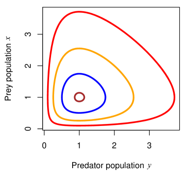
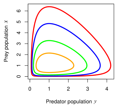
Figure 1: Left panel: with $\alpha=1$ and $H(x,y)=3.40,2.61,2.19$, and $2.01$. Right panel: with $\alpha=0.5,0.6,0.8$, and $1.2$, from outside inward, all with $H(x,y)=2.61$. We see that the larger the $\alpha$, the smaller the temporal variations in the prey population, relative to that of predator.

It is easy to check that the solutions to (1) in phase space are level curves of a scalar function [1]

$$H(x,y)=\alpha x+y-\ln\big{(}x^{\alpha}y\big{)}.$$ (2)

We shall use $\Gamma_{H=h}$ to denote the solution curve $H(x,y)=h$, and $\mathfrak{D}_{h}(\alpha)$ to denote the domain encircled by the $\Gamma_{H=h}$. Fig. 1 shows the contours of $H(x,y)$ with $\alpha=1$ and $H(x,y)=2.61$ with different $\alpha$’s.

Let $\tau$ be the period of the cyclic dynamics. Then it is easy to show that [1]

$$\frac{1}{\tau}\int_{0}^{\tau}x(t){\rm d}t=\frac{1}{\tau}\int_{0}^{\tau}y(t){\rm d}t=1.$$ (3)

Furthermore (see Appendix A),

$$\frac{1}{\tau}\int_{0}^{\tau}\big{(}x(t)-1\big{)}^{2}{\rm d}t=\frac{\hat{\mathcal{A}}}{\alpha\tau},$$ (4)

$$\frac{1}{\tau}\int_{0}^{\tau}\big{(}y(t)-1\big{)}^{2}{\rm d}t=\frac{\alpha\hat{\mathcal{A}}}{\tau},$$ (5)

in which $\hat{\mathcal{A}}$ is the area of $\mathfrak{D}_{h}(\alpha)$, encircled by $\Gamma_{H=h}$, using Lebesgue measure in the $xy$-plane. The appropriate measure for computing the area will be further discussed in Sec. 2. The parameter $\alpha$ represents the relative temporal variations, or dynamic ranges, in the two populations: the larger the $\alpha$, the greater the temporal variations and range in the predator population, and the smaller in the prey population.

The paper is organized as follows. In Sec. 2, an extended conservation law is recognized for the Lotka-Volterra system. Then the relationship among three quantities: the “energy” function $H(x,y)$, the area $\mathcal{A}$ encircled by the level set $\Gamma_{H=h}$, and the parameter $\alpha$ is developed. According to the Helmholtz theorem, the conjugate variables of $\mathcal{A}$ and $\alpha$ are found as time averages of certain functions of population $x(t)$ and $y(t)$. Analysis on those novel “state variables” demonstrates the tendency of change in mean ecological quantities like population range or ecological activeness when the parameter $\alpha$ or energy $H$ varies. In Sec. 3, we show that the area $\mathcal{A}$ encircled by $\Gamma_{H=h}$ is related to the concept of entropy. In Sec. 4, the conservative dynamics is shown to be an integral part of the stochastic population dynamics, which necessarily has the same invariant density as the deterministic conservative dynamics. In the large population limit, a separation of time scale between the fast cyclic motion on $\Gamma_{H=h}$ and the slow stochastic crossing of $\Gamma_{H=h}$ is observed in the stochastic dynamical system. The paper concludes with a discussion in Sec. 5.

2 The Helmholtz theorem

Eq. (1) is not a Hamiltonian system, nor is it divergence-free

$$\frac{\partial f(x,y)}{\partial x}+\frac{\partial g(x,y;\alpha)}{\partial y}\neq 0.$$

It can be expressed, however, as

$$\frac{{\rm d}x}{{\rm d}t}=-G(x,y)\frac{\partial H(x,y)}{\partial y},\ \ \ \frac{{\rm d}y}{{\rm d}t}=G(x,y)\frac{\partial H(x,y)}{\partial x},$$ (6)

with a scalar factor $G(x,y)=xy$. One can in fact understand this scalar factor as a “local change of measure”, or time ${\rm d}\hat{t}\equiv G\big{(}x(t),y(t)\big{)}{\rm d}t$ [8]:

$$x(t)=\hat{x}\big{(}\hat{t}(t)\big{)},\ \ y(t)=\hat{y}\big{(}\hat{t}(t)\big{)},$$ (7)

for

$$\hat{t}(t)=\hat{t}_{0}+\int_{t_{0}}^{t}G\big{(}x(s),y(s)\big{)}{\rm d}s,$$

where $(\hat{x},\hat{y})$ satisfies the corresponding Hamiltonian system. In Sec. 3 and 4 below, we shall show that $G^{-1}(x,y)$ is an invariant density of the Liouville equation for the deterministic dynamics (1), and more importantly the invariant density of the Fokker-Planck equation for the corresponding stochastic dynamics. As will be demonstrated in Sec. 2.2 and 2.3, statistical average of quantities according to the invariant measure $G^{-1}(x,y){\rm d}x{\rm d}y$ can be calculated through time average of those quantities along the system’s instantaneous dynamics. Knowledge about the system’s long term distribution is not needed during the calculation. These facts make the $G^{-1}(x,y)$ the natural measure for computing area $\mathcal{A}$.

Any function of $H(x,y)$, $\rho(H)$ is conserved under the dynamics, as is guaranteed by the orthogonality between the vector field of (1) and gradient $\nabla\rho$ [9]:

$$\frac{{\rm d}\rho\big{(}H(x,y)\big{)}}{{\rm d}t} = f(x,y)\frac{\partial}{\partial x}\rho\big{(}H(x,y)\big{)}+g(x,y;\alpha)\frac{\partial}{\partial y}\rho\big{(}H(x,y)\big{)}$$ (8)

$$= \rho^{\prime}(H)\left(x(1-y)\alpha\left(1-\frac{1}{x}\right)+\alpha y(x-1)\left(1-\frac{1}{y}\right)\right)$$

$$= 0.$$

This is analogous to the “conservation law” observed in Hamiltonian systems.

2.1 Extending the conservation law

The nonlinear dynamics in (1), therefore, introduces a “conservative relation” between the populations of predator and prey according to (2). If we call the value $H(x,y)$ an “energy”, then the phase portrait in the left panel of Fig. 1 suggests that the entire phase space of the dynamical system is organized according to the value of $H$. The deep insight contained in the work of Helmholtz and Boltzmann [10, 12] is that such an energy-based organization can be further extended for different values of $\alpha$: Therefore, the energy-based organization is no longer limited to a single orbit, nor a single dynamical system; but rather for the entire class of parametric dynamical systems. In the classical physics of Newtonian mechanical energy conservation, this yields the mechanical basis of the Fundamental Thermodynamic Relation as a form of the First Law, which extends the notion of energy conservation far beyond mechanical systems [15, 16].

More specifically, we see that the area $\mathcal{A}$ in Fig. 1, or in fact any geometric quantification of a closed orbit, is completely determined by the parameter $\alpha$ and initial energy value $h=H\big{(}x(0),y(0),\alpha\big{)}$. Therefore, there must exist a bivariate function $\mathcal{A}=\mathcal{A}(h,\alpha)$, Assuming the implicit function theorem applies, then one has

$$h=h(\mathcal{A},\alpha).$$ (9)

Note that in terms of the Eq. (9), a “state” of the ecological system is not a single point $(x,y)$ which is continuously varying with time; rather it reflects the geometry of an entire orbit. Then Eq. (9) implies that any such ecological state has an “h-energy”, if one recognizes a geometric, state variable $\mathcal{A}$.

Eq. (9) can be written in a differential form

$${\rm d}h=\left(\frac{\partial h}{\partial\mathcal{A}}\right)_{\alpha}{\rm d}\mathcal{A}+\left(\frac{\partial h}{\partial\alpha}\right)_{\mathcal{A}}{\rm d}\alpha,$$ (10)

in which one first introduces the h-energy for an ecological system with fixed $\alpha$ via the factor $(\partial h/\partial\mathcal{A})$. Then, holding $\mathcal{A}$ constant, one introduces an “$\alpha$-force” corresponding to the parameter $\alpha$. In classical thermodynamics, the latter is known as an “adiabatic” process.

The Helmholtz theorem expresses the two partial derivatives in (10) in terms of the dynamics in Eq. (1).

2.2 Projected invariant measure

For canonical Hamiltonian systems, Lebesgue measure is an invariant measure in the whole phase space. On the level set $\Gamma_{H=h}$, the projection of the Lebesgue measure, called the Liouville measure, also defines an invariant measure on the sub-manifold. If the dynamics on the invariant sub-manifold $\Gamma_{H=h}$ is ergodic, the average with respect to the Liouville measure is equal to the time average along the trajectory starting from any initial condition $(x_{0},y_{0})$ satisfying $H(x_{0},y_{0})=h$.

As we shall show below, the invariant measure for the LV system (1) in the whole phase space is ${\rm d}\mathcal{A}=G^{-1}(x,y){\rm d}x{\rm d}y$. Projection of this invariant measure onto the level set $\Gamma_{H=h}$ can be found by changing $(x,y)$ to intrinsic coordinates $(h,\ell)$:

$${\rm d}\mathcal{A}=G^{-1}(x,y)\ {\rm d}x{\rm d}y=G^{-1}(x,y)\ \big{(}{\rm d}x,{\rm d}y\big{)}^{T}\cdot\mathbf{n}\ {\rm d}\ell,$$ (11)

where

$$\mathbf{n}=\left(\dfrac{\partial H(x,y)/\partial x}{||\nabla H(x,y)||},\dfrac{\partial H(x,y)/\partial y}{||\nabla H(x,y)||}\right)_{(x,y)\in\Gamma_{H=h}}^{T}$$ (12)

is the unit normal vector of the the level set $\Gamma_{H=h}$; and ${\rm d}\ell=\sqrt{{\rm d}x^{2}+{\rm d}y^{2}}$. Noting that:

$${\rm d}h = \dfrac{\partial H(x,y)}{\partial x}{\rm d}x+\dfrac{\partial H(x,y)}{\partial y}{\rm d}y,$$ (13)

we have

$$\big{(}{\rm d}x,{\rm d}y\big{)}^{T}\cdot\mathbf{n}=\dfrac{{\rm d}h}{||\nabla H(x,y)||}.$$ (14)

That is:

$${\rm d}\mathcal{A}={\rm d}\mu\ {\rm d}h,$$ (15)

where

$${\rm d}\mu=\dfrac{G^{-1}(x,y)}{||\nabla H(x,y)||}{\rm d}\ell$$ (16)

is the projected invariant measure of the Lotka-Volterra system on the level set $\Gamma_{H=h}$.

It is worth noting that ${\rm d}\mu={\rm d}t$ on the level set $\Gamma_{H=h}$. Since dynamics on $\Gamma_{H=h}$ is ergodic, the average of any function $\psi(x,y)$ under the projected invariant measure on $\Gamma_{H=h}$ is equal to its time average over a period:

$$\langle\psi\rangle^{\Gamma_{H=h}} \triangleq\frac{\displaystyle\oint_{\Gamma_{H=h}}\psi\big{(}x,y\big{)}{\rm d}\mu}{\displaystyle\oint_{\Gamma_{H=h}}{\rm d}\mu}$$

$$=\frac{1}{\tau}\int_{0}^{\tau}\psi\big{(}x(t),y(t)\big{)}{\rm d}t\triangleq\langle\psi\rangle^{t}$$ (17)

2.3 Functional relation between $\ln\mathcal{A}$, $\alpha$, and $h$

Under the invariant measure $G^{-1}(x,y)$, the area $\mathcal{A}$ encircled by the level curve $\Gamma_{H=h}$ is:

$$\mathcal{A}_{\mathfrak{D}_{h}(\alpha)} = \iint_{\mathfrak{D}_{h}(\alpha)}G^{-1}(x,y){\rm d}x{\rm d}y$$ (18)

$$= \iint_{\mathfrak{D}_{h}(\alpha)}{\rm d}\ln x\ {\rm d}\ln y$$

Using Green’s theorem the area $\mathcal{A}_{\mathfrak{D}_{h}(\alpha)}$ can be simplified as

$$\mathcal{A}_{\mathfrak{D}_{h}(\alpha)} = \int_{0}^{\tau(h,\alpha)}\ln y\left(\frac{\partial H}{\partial\ln y}\right){\rm d}t$$ (19)

$$= \int_{0}^{\tau(h,\alpha)}\ln x\left(\frac{\partial H}{\partial\ln x}\right){\rm d}t,$$

where $\tau(h,\alpha)$ is the time period for the cyclic motion. Furthermore,

$$\frac{\partial\mathcal{A}_{\mathfrak{D}_{h}(\alpha)}}{\partial h} = \frac{\partial}{\partial h}\iint_{\mathfrak{D}_{h}(\alpha)}G^{-1}(x,y)\ {\rm d}x{\rm d}y$$ (20)

$$= \int_{0}^{\tau(h,\alpha)}{\rm d}t=\tau(h,\alpha).$$

That is

$$\left(\frac{\partial\ln\mathcal{A}_{\mathfrak{D}_{h}(\alpha)}}{\partial h}\right)^{-1}=\left\langle\ln x\left(\frac{\partial H}{\partial\ln x}\right)\right\rangle^{t}=\left\langle\ln y\left(\frac{\partial H}{\partial\ln y}\right)\right\rangle^{t},$$ (21)

in which $\langle\cdots\rangle^{t}$ is the time average, or phase space average according to the invariant measure. We can also find the derivative of the area $\mathcal{A}_{\mathfrak{D}_{h}(\alpha)}$ encircled by the level curve $\Gamma_{H=h}$ with respect to the parameter of the system $\alpha$ as:

$$\frac{\partial\mathcal{A}_{\mathfrak{D}_{h}(\alpha)}}{\partial\alpha} = \frac{\partial}{\partial\alpha}\iint_{\mathfrak{D}_{h}(\alpha)}G^{-1}(x,y)\ {\rm d}x{\rm d}y$$ (22)

$$= -\int_{0}^{\tau(h,\alpha)}\big{(}x(t)-\ln{x(t)}\big{)}\ {\rm d}t.$$

In this setting, the Helmholtz theorem reads

$${\rm d}h=\frac{\displaystyle{\rm d}\mathcal{A}-\left(\frac{\partial\mathcal{A}}{\partial\alpha}\right)_{h}{\rm d}\alpha}{\displaystyle\left(\frac{\partial\mathcal{A}}{\partial h}\right)_{\alpha}}=\theta(h,\alpha)\ {\rm d}\ln\mathcal{A}-F_{\alpha}(h,\alpha){\rm d}\alpha,$$ (23)

in which

$$\theta(h,\alpha)=\mathcal{A}_{\mathfrak{D}_{h}(\alpha)}\left(\frac{\partial\mathcal{A}}{\partial h}\right)_{\alpha}^{-1}=\left\langle\ln x\left(\frac{\partial H}{\partial\ln x}\right)\right\rangle^{t}=\left\langle\ln y\left(\frac{\partial H}{\partial\ln y}\right)\right\rangle^{t}.$$ (24)

The factor $\theta(h,\alpha)$ here is the mean $\ln x(\partial H/\partial\ln x)$, or $\ln y(\partial H/\partial\ln y)$, precisely like the mean kinetic energy as the notion of temperature in classical physics, and the virial theorem. The $\alpha$-force is then defined as

$$F_{\alpha}(h,\alpha)=\left(\frac{\partial\mathcal{A}}{\partial\alpha}\right)_{h}\left(\frac{\partial\mathcal{A}}{\partial h}\right)_{\alpha}^{-1}=-\left\langle\frac{\partial H(x,y,\alpha)}{\partial\alpha}\right\rangle^{t}.$$ (25)

It is important to note that the definition of $F_{\alpha}$ given in the right-hand-side of (25) is completely independent of the notion of $\mathcal{A}$, even though the relation (23) explicitly involves the latter. $F_{\alpha}(h,\alpha)$ is a function of both $h$ and $\alpha$, however. Therefore, the value of $\alpha$-work $F_{\alpha}(h,\alpha){\rm d}\alpha$ depends on how $h$ is constrained: There are iso-$h$ processes, iso-$\theta$ processes, etc. [20]

2.4 Equation of state

The notion of an equation of state first appeared in classic thermodynamics [15, 16]. From a modern dynamical systems standpoint, a fixed point as a function usually is continuously dependent upon the parameters in a mathematical model, except at bifurcation points. Let $(x_{1}^{*},x_{2}^{*},\cdots,x_{n}^{*})$ be a globally asymptotically attractive fixed point, and $\alpha$ be a parameter, then the function $x_{1}^{*}(\alpha)$ constitutes an equation of state for the long-time “equilibrium” behavior of the dynamical system.

If a system has a globally asymptotically attractive limit set that is not a simple fixed point, then every geometric characteristic of the invariant manifold, say $\mathfrak{g}^{*}$, will be a function of $\alpha$. In this case, $\mathfrak{g}^{*}(\alpha)$ could well be considered as an equation of state. An “equilibrium state” in this case is the entire invariant manifold.

The situation for a conservative dynamical system with center manifolds is quite different. In this case, the long-time behavior of the dynamical system, the foremost, is dependent upon its initial data. An equation of state therefore is a functional relation among (i) geometric characteristics of a center manifold $\mathfrak{g}^{*}$, (ii) parameter $\alpha$, and (iii) a new quantity, or quantities, that identifies a specific center manifold, $h$. This is the fundamental insight of the Helmholtz theorem.

In ecological terms, area under the invariant measure: $\mathcal{A}$, gives a sense of total variation in both the predator’s and the prey’s populations. Therefore, $\ln\mathcal{A}$ measures population range of both populations as a whole. The parameter $\alpha$, on the other hand, is the proportion of predators’ over preys’ population ranges of time variations:

$$\alpha^{2}=\dfrac{\int_{0}^{\tau(h,\alpha)}\big{(}y(t)-1\big{)}^{2}{\rm d}t}{\int_{0}^{\tau(h,\alpha)}\big{(}x(t)-1\big{)}^{2}{\rm d}t}=\dfrac{\left\langle(y-1)^{2}\right\rangle^{t}}{\left\langle(x-1)^{2}\right\rangle^{t}}.$$ (26)

The new quantity $\theta$ can be viewed as a measure of the mean ecological “activeness”:

$$\theta=\left\langle\alpha(x-1)\ln x\right\rangle^{t}=\left\langle(y-1)\ln y\right\rangle^{t}.$$ (27)

It is the mean of “distance” from the prey’s and predator’s populations $x$ and $y$, to the fixed populations in equilibrium $(1,1)$. For population dynamic variable $u$, Eq. 27 suggests a norm $\|u\|\equiv u\ln(u+1)$. Then, $\theta=\left\langle\alpha\|x-1\|\right\rangle^{t}=\left\langle\|y-1\|\right\rangle^{t}$; and an averaged norm of per capita growth rates in the two species:

$$\theta=\left\langle\alpha\left\|\frac{1}{\alpha}\dfrac{{\rm d}\ln y}{{\rm d}t}\right\|\right\rangle^{t}=\left\langle\left\|-\dfrac{{\rm d}\ln x}{{\rm d}t}\right\|\right\rangle^{t}.$$ (28)

And finally,

$$F_{\alpha}=-\left\langle\dfrac{\partial H(x,y,\alpha)}{\partial\alpha}\right\rangle^{t}=-\left\langle x-\ln x\right\rangle^{t}$$ (29)

is the “ecological force” one needs to counteract in order to change $\alpha$. In other words, when $|F_{\alpha}|$ is greater, more $h$-energy change is needed to vary $\alpha$. It is also worth noting that $|F_{\alpha}|$ is positively related to the prey’s average population range. In fact we can define another “distance” of the prey’s population $x$ to $1$ as: $\|u\|_{F}=u-\ln(u+1)$, then $F_{\alpha}=-\big{\langle}\|x-1\|_{F}\big{\rangle}^{t}-1$. Note that for very small $u$: $\|u\|\approx u^{2}\approx 2\|u\|_{F}$

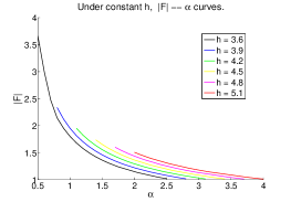
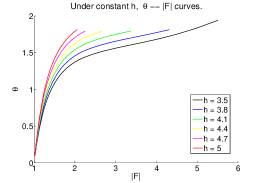
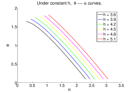
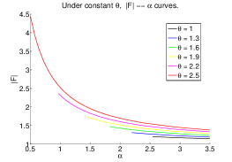
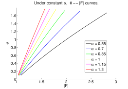
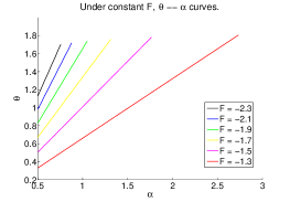
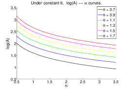
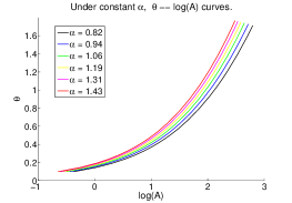
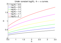
Figure 2: Various functional relationships, e.g., “the equation of state”, among $\big{(}|F|,\alpha,h\big{)}$, $\big{(}|F|,\theta,h\big{)}$, and $\big{(}\theta,\alpha,h\big{)}$ in the top row, different views among $\big{(}|F|,\theta,\alpha\big{)}$ in the second row, and among $\big{(}\ln(\mathcal{A}),\theta,\alpha\big{)}$ in the third row.

Fig. 2 shows various forms of “the equation of state”, e.g., relationships among the triplets $\big{(}\alpha,|F_{\alpha}|=-F_{\alpha},h\big{)}$, $\big{(}|F_{\alpha}|,\theta,h\big{)}$, and $\big{(}\alpha,\theta,h\big{)}$ in the first row; among the triplet $\big{(}\alpha,|F_{\alpha}|,\theta\big{)}$ in the second row; and among the triplet $\big{(}\mathcal{A},\theta,\alpha\big{)}$ in the third row. The second row shows that the relation among $\big{(}\alpha,|F_{\alpha}|,\theta\big{)}$ is just like that among $\big{(}V,P,T\big{)}$ in ideal gas model: Mean ecological activeness $\theta$ increases nearly linearly with the ecological force $|F_{\alpha}|$ for constant $\alpha$, and with the proportion $\alpha$ of the predator’s population range over the prey’s, for constant $|F_{\alpha}|$; Ecological force $|F_{\alpha}|$ and the proportion $\alpha$ of population ranges are inversely related under constant mean activeness $\theta$. And when $\theta=0$, $\alpha(F_{\alpha}+1)=0$. Other features can be observed by looking into the details of each column.

The first column of Fig. 2 demonstrates that as the proportion $\alpha$ of population ranges increases, the ecological force $|F_{\alpha}|$ is alleviated (for given $h$-energy or ecological activeness $\theta$). This is due to the positive relationship between the ecological force $|F_{\alpha}|$ and the prey’s population range (as shown in Eq. 29). Since $\alpha$ is the proportion of the predator’s population range over the prey’s, $|F_{\alpha}|$ and $\alpha$ would be inversely related when any resource, $h$-energy, or activity, $\theta$, remains constant. This fact means that on an iso-$h$ or iso-$\theta$ curve, when the proportion $\alpha$ is large, relatively less $h$-energy change is needed to reduce it. The first column also demonstrates an inverse relationship between $\alpha$ and the total population range $\ln\mathcal{A}$ for any given $\theta$, which reflects the fact that as the proportion of the predator’s population range over the prey’s increase, the total population range of the two species would actually decrease.

The second column of Fig. 2 demonstrates that: the ecological force $|F_{\alpha}|$ and the total population range $\ln\mathcal{A}$ increases with the mean activeness $\theta$ (with given $h$-energy or $\alpha$). This observation means that it would also take more $h$-energy to change the proportion $\alpha$ of the predator’s population range over the prey’s, if mean ecological activeness rises, and that more population range would be explored with more ecological activeness $\theta$.

The third column about the relation between $\theta$ and $\alpha$ is interesting: Under constant $h$-energy, as the proportion $\alpha$ of population ranges increases, the ecological activeness $\theta$ decreases, in accordance with the drop in the total population range $\ln\mathcal{A}$ as shown in Fig 1. But when the total population range $\ln\mathcal{A}$ or the ecological force $F_{\alpha}$ is to remain constant, ecological activeness $\theta$ actually increases with $\alpha$. This means that under constant resource ($h$-energy), the proportion $\alpha$ of the predator’s population range over the prey’s restricts mean ecological activeness. But if we fix the ecological force or total population range (supplying more $h$-energy), an increase in predator’s population range over prey’s can increase ecological activeness.

3 Liouville description in phase space

Nonlinear dynamics described by Eq. (1) has a linear, first-order partial differential equation (PDE) representation

$$\frac{\partial u(x,y,t)}{\partial t}=-\frac{\partial}{\partial x}\Big{(}f(x,y)u(x,y,t)\Big{)}-\frac{\partial}{\partial y}\Big{(}g(x,y;\alpha)u(x,y,t)\Big{)}.$$ (30)

A solution to (30) can be obtained via the method of characteristics, exactly via (1). Eq. (30) sometime is called the Liouville equation for the ordinary differential equations (1). It also has an adjoint:

$$\frac{\partial v(x,y,t)}{\partial t}=f(x,y)\frac{\partial v(x,y,t)}{\partial x}+g(x,y;\alpha)\frac{\partial v(x,y,t)}{\partial y}.$$ (31)

Note that while the orthogonality in Eq. (8) indicates that $\rho\big{(}H(x,y)\big{)}$ is a stationary solution to Eq. (31), it is not a stationary invariant density to (30).

This is due to the fact that vector field $(f,g)$ is not divergence free, but rather as in (6) the scalar factor $G(x,y)=xy$. Then it is easy to verify that $G^{-1}(x,y)\rho(H(x,y))$ is a stationary solution to (30):

$$\frac{\partial}{\partial x}\left(f(x,y)\ \frac{\rho(H(x,y))}{G(x,y)}\right)+\frac{\partial}{\partial y}\left(g(x,y)\ \frac{\rho(H(x,y))}{G(x,y)}\right)=0.$$ (32)

3.1 Entropy dynamics in phase space

It is widely known that a volume-preserving, divergence-free conservative dynamics has a conserved entropy $S[u(x,t)]=-\int_{\mathbb{R}}u(x,t)\ln u(x,t){\rm d}x$ [21]. For conservative system like (1) which contains the scalar factor $G(x,y)$, the Shannon entropy should be replaced by the relative entropy with respect to $G^{-1}(x,y)$ (see Appendix B for detailed calculation):

$$\frac{{\rm d}}{{\rm d}t}\int_{\mathbb{R}^{2}}u(x,y,t)\ln\left(\frac{u(x,y,t)}{G^{-1}(x,y)}\right){\rm d}x{\rm d}y=0.$$ (33)

Such systems are called canonical conservative with respect to $G^{-1}(x,y)$ in [8]. In classical statistical physics, the term $\int_{\mathbb{R}}u\ln\big{(}u/G^{-1}\big{)}{\rm d}x$ is called free energy [22]; in information theory, Kullback-Leibler divergence.

We can in fact show a stronger result, with arbitrary differentiable $\Psi(\cdot)$ and $\rho(\cdot)$ over an arbitrary domain $\mathfrak{D}$ (see Appendix B):

$$\frac{{\rm d}}{{\rm d}t}\int_{\mathfrak{D}}u(x,y,t)\Psi\left(\frac{u(x,y,t)}{G^{-1}(x,y)\rho(H(x,y))}\right){\rm d}x{\rm d}y$$ (34)

$$= \int_{\partial\mathfrak{D}}\left\{u(x,y,t)\Psi\left(\frac{u(x,y,t)}{G^{-1}(x,y)\rho(H)}\right)\big{(}f,g\big{)}\right\}\times({\rm d}x,{\rm d}y).$$

Therefore, if $\mathfrak{D}=\mathfrak{D}_{h}$, then $\partial\mathfrak{D}=\Gamma_{H=h}$, and the integral on the right-hand-side of (34) is always zero. In other words, in conservative dynamics like (1), it is the support $\mathfrak{D}\subset\mathbb{R}^{2}$ on which $u(x,y,t)$ is observed that determines whether a system is invariant; not the initial data $u(x,y,0)$ [9].

3.2 Relation between $\mathcal{A}$, Shannon entropy, and relative entropy

Since a “state” is defined as an entire orbit, it is natural to change the coordinates from $(x,y)$ to $(h,s)$ according to the solution curve to (1), where we use $s$ to denote time, $0\leq s\leq\tau(h,\alpha)$. We have

$$\left(\frac{\partial x}{\partial t}\right)_{H=h}=x(1-y),\ \ \left(\frac{\partial y}{\partial t}\right)_{H=h}=\alpha y(x-1);$$ (35)

$$\left(\frac{\partial x}{\partial h}\right)_{s}\left(\alpha-\frac{\alpha}{x}\right)+\left(\frac{\partial y}{\partial h}\right)_{s}\left(1-\frac{1}{y}\right)=1.$$ (36)

Therefore:

$$\det\left[\frac{D(x,y)}{D(h,s)}\right]=xy=G(x,y).$$ (37)

Then, the generalized relative entropy can be expressed as

$$\int_{\mathfrak{D}_{h}}u(x,y,t)\Psi\left(\frac{u(x,y,t)}{G^{-1}(x,y)\rho(H(x,y))}\right){\rm d}x{\rm d}y$$ (38)

$$= \int_{h_{min}}^{h}{\rm d}\eta\int_{0}^{\tau(\eta,\alpha)}\frac{u\big{(}x(s),y(s),t\big{)}}{G^{-1}\big{(}x(s),y(s)\big{)}}\Psi\left(\frac{u\big{(}x(s),y(s),t\big{)}}{G^{-1}\big{(}x(s),y(s)\big{)}\rho(\eta)}\right){\rm d}s$$

$$= \int_{h_{min}}^{h}\rho(\eta){\rm d}\eta\int_{0}^{\tau(\eta,\alpha)}\widetilde{u}\big{(}x(s),y(s),t;\eta\big{)}\Psi\Big{(}\widetilde{u}\big{(}x(s),y(s),t;\eta\big{)}\Big{)}{\rm d}s$$

$$= \int_{h_{min}}^{h}\Omega_{B}(\eta)\rho(\eta){\rm d}\eta,$$

in which

$$\widetilde{u}(x,y,t;h)=\frac{u\big{(}x,y,t\big{)}}{G^{-1}\big{(}x,y\big{)}\rho(h)}.$$

and

$$\Omega_{B}(h)=\oint_{\Gamma_{H=h}}\widetilde{u}\big{(}x,y,0;h\big{)}\Psi\Big{(}\widetilde{u}\big{(}x,y,0;h\big{)}\Big{)}{\rm d}\ell.$$ (39)

$\Omega_{B}(h)$ is known as Boltzmann’s entropy in classical statistical mechanics. We see that the $\mathcal{A}$ introduced in Sec. 2 is the simplest case of the generalized relative entropy in (34) with $\rho=\Psi=1$, and $u(x,y,0)=G^{-1}(x,y)$. Then $\Omega_{B}(h)={\rm d}\mathcal{A}_{\mathfrak{D}_{h}}/{\rm d}h$. Gibbs’ canonical ensemble chooses $\rho(h)=e^{-h/\theta}$.

The dynamics (1) is not ergodic in the $xy$-plane; it does not have a unique invariant measure, as indicated by the arbitrary $\rho(H)$ in Eq. (32). However, the function $G(x,y)$, as indicated in Eqs. (2) and (37), is the unique invariant measure on each ergodic invariant submanifold $\Gamma_{H=h}$. It is non-uniform with respect to Lebesgue measure. On the ergodic invariant manifold $\Gamma_{H=h}$: $G(x,y){\rm d}t\leftrightarrow{\rm d}\ell$. To see the difference between the Lebesgue-based average and invariant-measure based average, consider a simple time-varying exponentially growing population: $\frac{{\rm d}u(t)}{{\rm d}t}=r(t)u(t)$. The regular time average of the per capita growth rate is

$$\frac{1}{\tau}\int_{0}^{\tau}\frac{1}{u(t)}\frac{{\rm d}u}{{\rm d}t}{\rm d}t=\frac{1}{\tau}\ln\left(\frac{u(\tau)}{u(0)}\right)=\frac{1}{\tau}\int_{0}^{\tau}r(t)dt.$$

The Lebesgue-based average is an “average growth rate per average capita”

$$\frac{\displaystyle\int_{0}^{\tau}\frac{1}{u(t)}\frac{{\rm d}u}{{\rm d}t}\ u(t){\rm d}t}{\displaystyle\int_{0}^{\tau}u(t){\rm d}t}=\frac{\displaystyle\int_{0}^{\tau}r(t)u(t){\rm d}t}{\displaystyle\int_{0}^{\tau}u(t){\rm d}t}.$$

In cyclic population dynamics, this latter quantity corresponds to the $G\big{(}x(t),y(t)\big{)}$ weighted per capita growth rate or “kinetic energy”

$$\frac{\displaystyle\int_{0}^{\tau(h,\alpha)}\left(\frac{{\rm d}\ln(y)}{{\rm d}t}\right)G\big{(}x(t),y(t)\big{)}{\rm d}t}{\displaystyle\int_{0}^{\tau(h,\alpha)}G\big{(}x(t),y(t)\big{)}{\rm d}t}=\frac{\displaystyle\int_{0}^{\tau(h,\alpha)}-\left(\frac{{\rm d}\ln(x)}{{\rm d}t}\right)G\big{(}x(t),y(t)\big{)}{\rm d}t}{\displaystyle\int_{0}^{\tau(h,\alpha)}G\big{(}x(t),y(t)\big{)}{\rm d}t}$$

$$= \frac{\displaystyle\int_{0}^{\tau(h,\alpha)}x\left(\frac{\partial H}{\partial x}\right)G\big{(}x(t),y(t)\big{)}{\rm d}t}{\displaystyle\int_{0}^{\tau(h,\alpha)}G\big{(}x(t),y(t)\big{)}{\rm d}t}=\frac{\displaystyle\int_{0}^{\tau(h,\alpha)}y\left(\frac{\partial H}{\partial y}\right)G\big{(}x(t),y(t)\big{)}{\rm d}t}{\displaystyle\int_{0}^{\tau(h,\alpha)}G\big{(}x(t),y(t)\big{)}{\rm d}t}.$$ (40)

4 Stochastic description of finite populations

In this section, we show that the conservative dynamics in (1) is an emergent caricature of a robust stochastic population dynamics. This material can be found in many texts, e.g., [19]. But for completeness, we shall give a brief summary.

Assume the populations of the prey and the predator, $M(t)$ and $N(t)$, reside in a spatial region of size $\Omega$. The discrete stochastic population dynamics follows a two-dimensional, continuous time birth-death process with transition probability rate

$$\Pr\Big{\{}M(t+\Delta t)=k,N(t+\Delta t)=\ell\ \Big{|}M(t)=m,N(t)=n\Big{\}}$$ (41)

$$= \left(m\delta_{k,m+1}+\dfrac{1}{\Omega}mn\delta_{k,m-1}+\dfrac{\alpha}{\Omega}nm\delta_{\ell,n+1}+\alpha n\delta_{\ell,n-1}\right)\Delta t+o(\Delta t).$$

The discrete stochastic dynamics has an invariant measure:

$${\rm Pr}^{ss}\Big{\{}M=m,N=n\Big{\}}=\dfrac{1}{mn}.$$ (42)

Then

$$p_{m,n}(t+\Delta t) = p_{m,n}(t)\left[1-\left(m+\dfrac{1}{\Omega}mn+\dfrac{\alpha}{\Omega}nm+\alpha n\right)\Delta t\right]$$

$$+ p_{m-1,n}(t)\Big{[}(m-1)\Delta t\Big{]}+p_{m+1,n}(t)\left[\dfrac{1}{\Omega}(m+1)n\Delta t\right]$$

$$+ p_{m,n-1}(t)\left[\dfrac{\alpha}{\Omega}(n-1)m\Delta t\right]+p_{m,n+1}(t)\Big{[}\alpha(n+1)\Delta t\Big{]}.$$

That is

$$\dfrac{p_{m,n}(t+\Delta t)-p_{m,n}(t)}{\Delta t} = -m\Big{[}p_{m,n}(t)-p_{m-1,n}(t)\Big{]}-p_{m-1,n}(t)$$ (43)

$$+ \dfrac{1}{\Omega}mn\Big{[}p_{m+1,n}(t)-p_{m,n}(t)\Big{]}+\dfrac{1}{\Omega}np_{m+1,n}(t)$$

$$- \dfrac{\alpha}{\Omega}nm\Big{[}p_{m,n}(t)-p_{m,n-1}(t)\Big{]}-\dfrac{\alpha}{\Omega}mp_{m,n-1}(t)$$

$$+ \alpha n\Big{[}p_{m,n+1}(t)-p_{m,n}(t)\Big{]}+\alpha p_{m,n+1}(t).$$

For a very large $\Omega$, the population densities at time $t$ can be approximated by continuous random variables as $X(t)=\Omega^{-1}M(t)$ and $Y(t)=\Omega^{-1}N(t)$. Then Eq. (43) becomes a partial differential equation by setting $x=m/\Omega$, $y=n/\Omega$, and $u(x,y,t)=p_{m,n}(t)/\Omega$:

$$\dfrac{\partial u}{\partial t} = -x\dfrac{\partial u}{\partial x}+\dfrac{1}{2}\Omega^{-1}x\dfrac{\partial^{2}u}{\partial x^{2}}-u+\Omega^{-1}\dfrac{\partial u}{\partial x}$$

$$+ xy\dfrac{\partial u}{\partial x}+\dfrac{1}{2}\Omega^{-1}xy\dfrac{\partial^{2}u}{\partial x^{2}}+yu+\Omega^{-1}y\dfrac{\partial u}{\partial x}$$

$$- \alpha xy\dfrac{\partial u}{\partial y}+\dfrac{\alpha}{2}\Omega^{-1}xy\dfrac{\partial^{2}u}{\partial y^{2}}-\alpha xu+\alpha\Omega^{-1}x\dfrac{\partial u}{\partial y}$$

$$+ \alpha y\dfrac{\partial u}{\partial y}+\dfrac{\alpha}{2}\Omega^{-1}y\dfrac{\partial^{2}u}{\partial y^{2}}+\alpha u+\alpha\Omega^{-1}\dfrac{\partial u}{\partial y}+o(\Omega^{-1}).$$

Rearranging the terms and writing $\epsilon=\Omega^{-1}$, we can perform the Kramers-Moyal expansion to obtain:

$$\frac{\partial u(x,y,t)}{\partial t} = \nabla\cdot\Big{(}\epsilon{\bf D}(x,y)\nabla u-{\bf F}(x,y)u\Big{)}+\dfrac{\epsilon}{2}\left((y+1)\dfrac{\partial u}{\partial x}+\alpha(x+1)\dfrac{\partial u}{\partial y}\right)+o(\epsilon)$$ (44)

$$= \epsilon\sum_{\xi=x,y}\sum_{\zeta=x,y}\frac{\partial^{2}}{\partial\xi\partial\zeta}D_{\xi\zeta}(x,y)u(x,y,t)-\nabla\cdot\Big{(}{\bf F}(x,y)\ u\Big{)},$$

with drift ${\bf F}(x,y)=\big{(}f(x,y),g(x,y;\alpha)\big{)}^{T}$ and symmetric diffusion matrix

$${\bf D}(x,y)=\left(\begin{array}[]{cc}D_{xx}(x,y)&D_{xy}(x,y)\\ D_{yx}(x,y)&D_{yy}(x,y)\end{array}\right)=\frac{1}{2}\left(\begin{array}[]{cc}x(1+y)&0\\ 0&\alpha y(x+1)\end{array}\right).$$

Eq. (44) should be interpreted as a Fokker-Plank equation for the probability density function $u(x,y,t){\rm d}x{\rm d}y=\Pr\big{\{}x<X(t)\leq x+{\rm d}x,y<Y(t)\leq y+{\rm d}y\big{\}}$. It represents a continuous stochastic process $\big{(}X(t),Y(t)\big{)}$ following Itō integral [17, 18, 19]:

$${\rm d}X(t) = X(1-Y){\rm d}t+\epsilon^{\frac{1}{2}}\sqrt{X(1+Y)}\ {\rm d}W_{1}(t)$$

$${\rm d}Y(t) = \alpha Y(X-1){\rm d}t+\epsilon^{\frac{1}{2}}\sqrt{\alpha Y(X+1)}\ {\rm d}W_{2}(t)$$

It is important to recognize that in the limit of $\epsilon\rightarrow 0$, the dynamics described by Eq. (44) is reduced to that in Eq. (30), which is equivalent to Eq. (1) via the method of characteristics.

4.1 Potential-current decomposition

It can be verified that the stationary solution to (44) is actually $G^{-1}(x,y)=(xy)^{-1}$, which is consistent with the discrete case (cf. Eq. 42), and also a stationary solution to the Liouville equation Eq. (30).

As suggested in [7, 9], the right-hand-side of Eq. (44) has a natural decomposition:

$$\nabla\cdot\Big{(}\epsilon{\bf D}(x,y)\nabla u-{\bf F}(x,y)u\Big{)}+\dfrac{\epsilon}{2}\left((y+1)\dfrac{\partial u}{\partial x}+\alpha(x+1)\dfrac{\partial u}{\partial y}\right)$$ (46)

$$= \nabla\cdot\Big{[}\epsilon{\bf D}(x,y)\nabla u-\Big{(}{\bf F}(x,y)-\epsilon{\bf D}(x,y)\nabla\ln G(x,y)\Big{)}u\Big{]}$$

$$= \nabla\cdot\Big{[}\epsilon{\bf D}\Big{(}u\nabla\ln u+u\nabla\ln G\Big{)}-{\bf F}u\Big{]}$$

$$= \epsilon\nabla\cdot{\bf D}u\nabla\Big{(}\ln\big{(}G\ u\big{)}\Big{)}-\nabla\cdot\big{(}{\bf F}\ u\big{)}$$

in which the first term is a self-adjoint differential operator and the second is skew-symmetric [8]. The equation from the first line to the second uses the fact $\nabla\ln G=-\big{(}x^{-1},y^{-1}\big{)}$, thus ${\bf D}\nabla\ln G=-\frac{1}{2}\big{(}(y+1),\alpha(x+1)\big{)}$. In terms of the stochastic differential equation in divergence form, this decomposition corresponds to:

$$\left(\begin{array}[]{c}{\rm d}X\\[5.0pt] {\rm d}Y\end{array}\right)=-\epsilon{\bf D}\nabla\ln G+G\left(\begin{array}[]{c}-H_{y}\\[5.0pt] H_{x}\end{array}\right)+\epsilon^{\frac{1}{2}}\sqrt{2{\bf D}}\left(\begin{array}[]{c}{\rm d}W_{1}(t)\\[5.0pt] {\rm d}W_{2}(t)\end{array}\right).$$ (47)

Under this non-Itō interpretation of the stochastic differential equation, the finite population with fluctuations (i.e., $\epsilon\neq 0$) is unstable when $x,y>0$. The system behaves as an unstable focus as shown in Fig. 4. The eigenvalues at the fixed point $\big{(}1+\epsilon,1-\epsilon\big{)}$ are $\pm i\sqrt{\alpha}+\frac{1}{2}\epsilon(\alpha+1)$, corresponding to the unstable nature of the stochastic system.

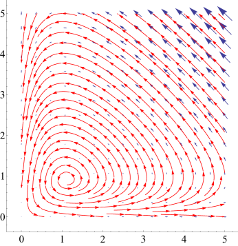
Figure 3: With fluctuation ($\epsilon=0.1$), the deterministic part of system (47). Red curves denote phase flow and blue arrows denote the strength of the vector field.

On the other hand, the potential-current decomposition reveals that the system (1) will be structurally stable in terms of the stochastic model: Any perturbation of the model system will yield corresponding conserved dynamics close to (1). The conservative ecology is a robust emergent phenomenon.

Equations such as (LABEL:sde) and (47) are not mathematically well-defined until an precise meaning of integration

$$X(t)=\int_{0}^{t}b\big{(}W(t)\big{)}{\rm d}W(t)$$ (48)

is prescribed. This yields different stochastic processes $X(t)$ whose corresponding probability density function $f_{X(t)}(x,t)$ follow different linear partial differential equations. The fundamental solution to any partial differential equation (PDE), however, provides a Markov transition probability; there is no ambiguity at the PDE level. On the other hand, the only interpretation of (48) that provides a Markovian stochastic process that is non-anticipating is that of Itō’s [23]. The differences in the interpretations of (48) become significant only in the modeling context, when one’s intuition expects that $E\big{[}X(t)\big{]}=0$ even for interpretations other then Itō’s.

4.2 The slowly fluctuating $H_{t}=H\big{(}X(t),Y(t)\big{)}$

With the $\big{(}X(t),Y(t)\big{)}$ defined in (44) and (LABEL:sde), let us now consider the stochastic functional

$${\rm d}H\big{(}X(t),Y(t)\big{)} = \alpha\left(1-\frac{1}{X}\right){\rm d}X+\left(1-\frac{1}{Y}\right){\rm d}Y+\frac{1}{2}\left(\frac{({\rm d}X)^{2}}{X^{2}}+\frac{({\rm d}Y)^{2}}{Y^{2}}\right)$$ (49)

$$= \alpha\epsilon^{\frac{1}{2}}\left(\frac{(X-1)^{2}(1+Y)}{X}+\frac{(Y-1)^{2}(X+1)}{Y}\right)^{\frac{1}{2}}{\rm d}W(t)$$

$$+\frac{\epsilon}{2}\left(\frac{(1+Y)}{X}+\frac{\alpha(X+1)}{Y}\right){\rm d}t$$

Therefore, for very large populations, i.e., small $\epsilon$, this suggests a separation of time scales between the cyclic motion on $\Gamma_{H=h}$ and slow, stochastic level crossing $H_{t}$. The method of averaging is applicable here [24, 25]:

$${\rm d}H_{t}=\epsilon b(H_{t}){\rm d}t+\epsilon^{\frac{1}{2}}A(H_{t}){\rm d}W(t),$$ (50)

with

$$b(h) = \frac{1}{2}\left\langle\frac{(1+y)}{x}+\frac{\alpha(x+1)}{y}\right\rangle^{\Gamma_{H=h}},$$ (51)

$$A(h) = \alpha\left\langle\left(\frac{(x-1)^{2}(1+y)}{x}+\frac{(y-1)^{2}(x+1)}{y}\right)^{\frac{1}{2}}\right\rangle^{\Gamma_{H=h}},$$ (52)

where $\left\langle\psi(x,y)\right\rangle^{\Gamma_{H=h}}=\left\langle\psi(x,y)\right\rangle^{t}$ denotes the average of $\psi(x,y)$ on the level set $\Gamma_{H=h}$. Then, using the Itō integral, the distribution of $H_{t}$ follows a Fokker-Planck equation:

$$\dfrac{\partial p(H,t)}{\partial t}=-\epsilon\dfrac{\partial}{\partial H}\big{(}b(H)p\big{)}+\dfrac{\epsilon}{2}\dfrac{\partial^{2}}{\partial H}\Big{(}A^{2}(H)p\Big{)}.$$ (53)

And the stationary solution for Eq. (53) is:

$$p^{ss}(H)=\dfrac{1}{A^{2}(H)}\exp\left({\displaystyle 2\int_{H_{0}}^{H}\dfrac{b(h)}{A^{2}(h)}{\rm d}h}\right).$$ (54)

The steady state distributions of $H$ under different $\alpha$’s are shown in Fig. 4. The steady state distribution $p^{ss}(H)$ does not depend on the volume size $\Omega=\epsilon^{-1}$.

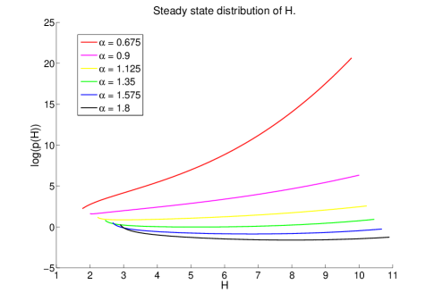
Figure 4: Under different values of $\alpha$, the steady state distribution $p^{ss}(H)$ with respect to $H$ in logarithmic scale. The slowly fluctuating “energy” $H$ ranges from $\alpha+1$ to infinity. Its steady state distribution $p^{ss}(H)$ eventually increases without bound as $H$ increases.

When $H$ is big enough, $p^{ss}(H)$ increases with $H$ without bound, since $b(H)$ is a positive increasing function. Hence, $p^{ss}(H)$ is not normalizable on the entire $\mathbb{R}$, reflecting the unstable nature of the system. The fluctuation $A(H)$ approaches zero when $H$ approaches $\alpha+1$. Consequently, the absorbing effect at $H=\alpha+1$ makes $p^{ss}(\alpha+1)$ another possible local maximum.

5 Discussion

It is usually an obligatory step in understanding an ODE $\dot{x}=f(x;\alpha,\beta)$ to analyze the dependence of a steady state $x^{*}$ as an implicit function of the parameters $(\alpha,\beta)$ [1]. One of the important phenomena in this regard is the Thom-Zeeman catastrophe [1, 26]. From this broad perspective, the analysis developed by Helmholtz and Boltzmann in 1884 is an analysis of the geometry of a “non-constant but steady solution”, as a function of its parameter(s) and initial conditions. In the context of LV equation (1), the geometry is characterized by the area encircled by a periodic solution, $\Gamma_{H=h}$, where $h$ is specified by the the initial data: $\mathcal{A}\big{(}\mathfrak{D}_{h}\big{)}=\mathcal{A}\big{(}h,\alpha\big{)}$. The celebrated Helmholtz theorem [10, 12] then becomes our Eq. (23)

$${\rm d}h=\frac{\displaystyle{\rm d}\mathcal{A}-\left(\frac{\partial\mathcal{A}}{\partial\alpha}\right)_{h}{\rm d}\alpha}{\displaystyle\left(\frac{\partial\mathcal{A}}{\partial h}\right)_{\alpha}}=\theta(h,\alpha)\ {\rm d}\ln\mathcal{A}-F_{\alpha}(h,\alpha){\rm d}\alpha.$$ (55)

Since Eq. (1) has a conserved quantity $H$, Eq. (55) can, and should be, interpreted as an extended $H$ conservation law, beyond the dynamics along a single trajectory, that includes both variations in $\alpha$ and in $h$. The partial derivatives in (55) can be shown as time averages of ecological activeness $\left\langle\ln x(\partial H/\partial\ln x)\right\rangle^{t}$ or $\left\langle\ln y(\partial H/\partial\ln y)\right\rangle^{t}$, and variation in the prey’s population $\left\langle x-\ln x\right\rangle^{t}$. Those conjugate variables, along with parameter $\alpha$, conserved quantity $H$, and encompassed area $\ln\mathcal{A}$ constitutes a set of “state variables” describing the state of an ecological system in its stationary, cyclic state. This is one of the essences of Boltzmann’s statistical mechanics [10].

For the monocyclic Lotka-Volterra system, the dynamics are relatively simple. Hence, the state variables have monotonic relationships, the same as that observed in ideal gas models. When the system’s dynamics become more complex (e.g. have more than one attractor, Hopf bifurcation), relations among the state variables will reflect that complexity (e.g. develop a cusp, exhibiting a phase transition in accordance [26]).

When the populations of predator and prey are finite, the stochastic predator-prey dynamics is unstable. This fact is reflected in the non-normalizable steady state distribution $G^{-1}(x,y)$ on $\mathbb{R}^{2+}$, and the destabilizing effect of the gradient dynamics in the potential-current decomposition. This is particular to the LV model we use; it is not a problem for the general theory if we study a more realistic model as in [27]. Despite the unstable dynamics, the stochastic model system is structurally stable: its dynamics persists under sufficiently small perturbations. This implies conservative dynamical systems like (1) are meaningful mathematical models, when interpreted correctly, for ecological realities.

Indeed, all ecological population dynamics can be represented by birth-death stochastic processes [19]. Except for systems with detailed balance, which rarely holds true, almost all such dynamics have underlying cyclic, stationary conservative dynamics. The present work shows that a hidden conservative ecological dynamics can be revealed through mathematical analyses. To recognize such a conservative ecology, however, several novel quantities need to be defined, developed, and becoming a part of ecological vocabulary. This is the intellectual legacy of Helmholtz’s and Boltzmann’s mechanical theory of heat [28].

Authors’ contributions. Y.-A. M. and H. Q. contributed equally to this work.

Competing interests. We declare there are no competing interests.

Acknowledgements. We thank R.E. O’Malley, Jr. and L.F. Thompson for carefully reading the manuscripts and many useful comments.

Appendix A Population temporal variations

$$\int_{0}^{\tau}\big{(}x(t)-1\big{)}^{2}{\rm d}t = \frac{1}{\alpha}\int_{0}^{\tau}\left(\frac{x-1}{y}\right){\rm d}y(t)$$ (A1)

$$= \frac{1}{\alpha}\int_{0}^{\tau}(x-1){\rm d}\Big{(}\alpha x(t)+y(t)-\alpha\ln x(t)\Big{)}$$

$$= \frac{1}{\alpha}\int_{0}^{\tau}(x-1){\rm d}y(t)$$

$$= \frac{1}{\alpha}\int_{0}^{\tau}x(t)\ {\rm d}y(t)\ =\ \frac{\hat{\mathcal{A}}}{\alpha}.$$

Similarly

$$\int_{0}^{\tau}\big{(}y(t)-1\big{)}^{2}{\rm d}t=-\alpha\int_{0}^{\tau}y(t)\ {\rm d}x(t)\ =\ \alpha\hat{\mathcal{A}}.$$ (A2)

Appendix B Dynamics of relative entropy and generalized relative entropy

Using the divergence theorem and noting that $\nabla\cdot\Big{(}G^{-1}f,G^{-1}g\Big{)}=0$, we obtain for the time evolution of the relative entropy:

$$\frac{{\rm d}}{{\rm d}t}\int_{\mathbb{R}^{2}}u(x,y,t)\ln\left(\frac{u(x,y,t)}{G^{-1}(x,y)}\right){\rm d}x{\rm d}y$$ (B1)

$$= \int_{\mathbb{R}^{2}}\frac{\partial u(x,y,t)}{\partial t}\left[\ln\left(\frac{u(x,y,t)}{G^{-1}(x,y)}\right)+1\right]{\rm d}x{\rm d}y$$

$$= -\int_{\mathbb{R}^{2}}\nabla\cdot\Big{(}(f,g)u(x,y,t)\Big{)}\ln\left(\frac{u(x,y,t)}{G^{-1}(x,y)}\right){\rm d}x{\rm d}y+\frac{\partial}{\partial t}\int_{\mathbb{R}^{2}}u(x,y,t){\rm d}x{\rm d}y$$

$$= -\int_{\mathbb{R}^{2}}\nabla\cdot\Big{(}(f,g)u(x,y,t)\Big{)}\ln\left(\frac{u(x,y,t)}{G^{-1}(x,y)}\right){\rm d}x{\rm d}y\$$

$$= -\int_{\mathbb{R}^{2}}\nabla\cdot\Big{(}G^{-1}f,G^{-1}g\Big{)}\times\left(\frac{u}{G^{-1}}\right)\ln\left(\frac{u}{G^{-1}}\right){\rm d}x{\rm d}y$$

$$-\int_{\mathbb{R}^{2}}\Big{(}G^{-1}f,G^{-1}g\Big{)}\cdot\nabla\left[\left(\frac{u}{G^{-1}}\right)\ln\left(\frac{u}{G^{-1}}\right)-\left(\frac{u}{G^{-1}}\right)\right]{\rm d}x{\rm d}y$$

$$= \int_{\mathbb{R}^{2}}\left[\left(\frac{u}{G^{-1}}\right)\ln\left(\frac{u}{G^{-1}}\right)-\left(\frac{u}{G^{-1}}\right)\right]\nabla\cdot\Big{(}G^{-1}f,G^{-1}g\Big{)}\ {\rm d}x{\rm d}y\ =\ 0.$$

A more general result can be obtained in parallel for arbitrary differentiable $\Psi(z)$ and $\rho(z)$:

$$\frac{{\rm d}}{{\rm d}t}\int_{\mathfrak{D}}u(x,y,t)\Psi\left(\frac{u(x,y,t)}{G^{-1}(x,y)\rho(H(x,y))}\right){\rm d}x{\rm d}y$$ (B2)

$$= \int_{\mathfrak{D}}\frac{\partial u(x,y,t)}{\partial t}\left[\Psi\left(\frac{u}{G^{-1}\rho(H)}\right)+\frac{u}{G^{-1}\rho(H)}\Psi^{\prime}\left(\frac{u}{G^{-1}\rho(H)}\right)\right]{\rm d}x{\rm d}y$$

$$= -\int_{\mathfrak{D}}\nabla\cdot\Big{(}(f,g)u\Big{)}\left[\Psi\left(\frac{u}{G^{-1}\rho(H)}\right)+\frac{u}{G^{-1}\rho(H)}\Psi^{\prime}\left(\frac{u}{G^{-1}\rho(H)}\right)\right]{\rm d}x{\rm d}y$$

$$= -\int_{\mathfrak{D}}\Big{(}G^{-1}\rho(H)f,G^{-1}\rho(H)g\Big{)}\cdot\nabla\left(\frac{u}{G^{-1}\rho(H)}\right)$$

$$\times\left[\Psi\left(\frac{u}{G^{-1}\rho(H)}\right)+\frac{u}{G^{-1}\rho(H)}\Psi^{\prime}\left(\frac{u}{G^{-1}}\rho(H)\right)\right]{\rm d}x{\rm d}y$$

$$= -\int_{\mathfrak{D}}\Big{(}G^{-1}\rho(H)f,G^{-1}\rho(H)g\Big{)}\cdot\nabla\left[\frac{u}{G^{-1}\rho(H)}\Psi\left(\frac{u}{G^{-1}\rho(H)}\right)\right]{\rm d}x{\rm d}y$$

$$= -\int_{\mathfrak{D}}\nabla\cdot\left\{\Big{(}G^{-1}\rho(H)f,G^{-1}\rho(H)g\Big{)}\left[\frac{u}{G^{-1}\rho(H)}\Psi\left(\frac{u}{G^{-1}\rho(H)}\right)\right]\right\}{\rm d}x{\rm d}y$$

$$= \int_{\partial\mathfrak{D}}\left\{u(x,y,t)\Psi\left(\frac{u(x,y,t)}{G^{-1}(x,y)\rho(H)}\right)\big{(}f,g\big{)}\right\}\times({\rm d}x,{\rm d}y).$$

References

- [1] Murray, J. D. (2002) Mathematical Biology I: An Introduction, 3rd ed., Springer, New York.
- [2] Kot, M. (2001) Elements of Mathematical Ecology, Cambridge Univ. Press, UK.
- [3] Qian, H. (2011) Nonlinear stochastic dynamics of mesoscopic homogeneous biochemical reaction systems - An analytical theory (Invited article). Nonlinearity, 24, R19–R49. (doi:10.1088/0951-7715/24/6/R01)
- [4] Zhang, X.-J., Qian, H. and Qian, M. (2013) Stochastic theory of nonequilibrium steady states and its applications. Part I. Phys. Rep. 510, 1–85. (doi:10.1016/j.physrep.2011.09.002)
- [5] Ao, P. (2005) Laws in Darwinian evolutionary theory (Review). Phys. Life Rev. 2, 117–156. (doi:10.1016/j.plrev.2005.03.002)
- [6] Qian, H., Qian, M. and Wang, J.-Z. (2012) Circular stochastic fluctuations in SIS epidemics with heterogeneous contacts among sub-populations. Theoret. Pop. Biol. 81, 223–231. (doi:10.1016/j.tpb.2012.01.002)
- [7] Wang, J., Xu, L. and Wang, E. (2008) Potential landscape and flux framework of nonequilibrium networks: Robustness, dissipation, and coherence of biochemical oscillations. Proc. Natl. Acad. Sci. USA 105, 12271–12276. (doi:10.1073/pnas.0800579105)
- [8] Qian, H. (2013) A decomposition of irreversible diffusion processes without detailed balance. J. Math. Phys. 54, 053302. (doi:10.1063/1.4803847)
- [9] Qian, H. (2014) The zeroth law of thermodynamics and volume-preserving conservative system in equilibrium with stochastic damping. Phys. Lett. A 378, 609–616. (doi:10.1016/j.physleta.2013.12.028)
- [10] Gallavotti, G. (1999) Statistical Mechanics: A Short Treatise, Springer, Berlin.
- [11] Khinchin, A. I. (1949) Mathematical Foundations of Statistical Mechanics, Dover, New York.
- [12] Campisi, M. (2005) On the mechanical foundations of thermodynamics: The generalized Helmholtz theorem. Studies in History and Philosophy of Modern Physics, 36, 275–290. (doi:10.1016/j.shpsb.2005.01.001)
- [13] Ma, Y.-A. and Qian, H. (2015) Universal ideal behavior and macroscopic work relation of linear irreversible stochastic thermodynamics. New J. Phys. 17, 065013. (doi:10.1088/1367-2630/17/6/065013)
- [14] Lotka, A. J. (1925) Elements of Physical Biology, Williams & Wilkins, Baltimore, MD.
- [15] Planck, M. (1969) Treatise on Thermodynamics, Dover, New York.
- [16] Pauli, W. (1973) Pauli Lectures on Physics: Thermodynamics and the Kinetic Theory of Gas, vol. 3, The MIT Press, Cambridge, MA.
- [17] Allen, L. J. S. (2010) An Introduction to Stochastic Processes with Applications to Biology, 2nd ed., Chapman & Hall/CRC, New York.
- [18] Grasman, J. and van Herwaarden, O. A. (1999) Asymptotic Methods for the Fokker-Planck Equation and the Exit Problem in Applications, Springer, Berlin.
- [19] Kurtz, T. G. (1981) Approximation of Population Processes. SIAM Pub, Philadelphia.
- [20] Qian, H. (2015) Thermodynamics of the general diffusion process: Equilibrium supercurrent and nonequilibrium driven circulation with dissipation. Eur. Phys. J. Special Topics, 224, 781–799. (doi:10.1140/epjst/e2015-02427-6)
- [21] Andrey, L. (1985) The rate of entropy change in non-Hamiltonian systems. Phys. Lett. A 111, 45–46. (doi:10.1016/0375-9601(85)90799-6)
- [22] Zhang, F., Xu, L., Zhang, K., Wang, E., and Wang, J. (2012) The potential and flux landscape theory of evolution. J Chem Phys. 137, 065102. (doi:10.1063/1.4734305)
- [23] Gardiner, C. W. (2004) Handbook of Stochastic Methods: For Physics, Chemistry and the Natural Sciences, 3rd ed., Springer-Verlag, Berlin.
- [24] Freidlin, M. I. and Wentzell, A. D. (2012) Random Perturbations of Dynamical Systems, 3rd ed., Springer-Verlag, New York.
- [25] Zhu, W.Q. (2006) Nonlinear stochastic dynamics and control in Hamiltonian formulation. Trans. A.S.M.E., 59, 230–248.
- [26] Ao, P., Qian, H., Tu, Y., and Wang, J. (2013) A theory of mesoscopic phenomena: Time scales, emergent unpredictability, symmetry breaking and dynamics across different levels, arXiv:1310.5585.
- [27] Xu, L., Zhang, F., Zhang, K., Wang, E., and Wang, J. (2014) The potential and flux landscape theory of ecology. PLoS ONE 9, e86746. (doi:10.1371/journal.pone.0086746)
- [28] Gallavotti, G., Reiter, W. L. and Yngvason, J. (2007) Boltzmann’s Legacy, ESI Lectures in Mathematics and Physics, Eur. Math. Soc. Pub., Züruch.