Relativistic effects in two-particle emission for electron and neutrino reactions

Abstract

Two-particle two-hole contributions to electroweak response functions are computed in a fully relativistic Fermi gas, assuming that the electroweak current matrix elements are independent of the kinematics. We analyze the genuine kinematical and relativistic effects before including a realistic meson-exchange current (MEC) operator. This allows one to study the mathematical properties of the non-trivial seven-dimensional integrals appearing in the calculation and to design an optimal numerical procedure to reduce the computation time. This is required for practical applications to CC neutrino scattering experiments, where an additional integral over the neutrino flux is performed. Finally we examine the viability of this model to compute the electroweak 2p-2h response functions.

I Introduction

The understanding of intermediate-energy (0.5–10 GeV) neutrino-nucleus scattering cross sections is an important ingredient to atmospheric and accelerator-based neutrino oscillation experiments Gal11 ; For12 ; Mor12 ; Alv14 . The analysis of these experiments requires having good control of nuclear effects. The simple description based on a relativistic Fermi gas (RFG) model does not accurately describe the recent measurements of quasielastic neutrino and antineutrino scattering Agu10 ; Agu13 ; Fio13 ; Abe13 . Mechanisms such as nuclear correlations, final-state interactions and Meson-exchange currents (MEC) may have an impact on the inclusive neutrino charged current (CC) cross section. In particular, explicit calculations support the theoretical evidence Mar09 ; Nie11 ; Ama11 for a significant contribution from multi-nucleon knock-out to the CC cross sections $(\nu_{\mu},\mu^{-})$ and $({\overline{\nu}}_{\mu},\mu^{+})$ around and above the quasielastic (QE) peak region, defined by $\omega=\sqrt{q^{2}+m_{N}^{2}}-m_{N}$, where $\omega$ is the energy transfer and $q$ is the 3-momentum transfer. Recent ab initio calculations Lov14 of sum rules of weak neutral-current response functions of ¹²C have also stressed the importance of MEC in neutrino quasielastic scattering. The size of MEC effects is larger than that found in inclusive CC neutrino scattering from the deuteron Shen12 .

The three existing microscopic models that have provided predictions of multi-nucleon knockout effects in quasielastic neutrino and antineutrino cross sections from ¹²C for the experimental kinematical settings are those by Martini Mar10 ; Mar11 ; Mar12 ; Mar13 ; Mar13b ; Mar14 , Nieves Nie11 ; Nie12 ; Nie13 ; Gra13 , and the Super-Scaling Analysis (SuSA) model of Ama11 ; Ama12 ; Ama13 .

These three models are based on the Fermi gas but each one contains different ingredients and approximations to face the problem. The Martini model is based on the non-relativistic model of Alb84 although attempts to improve it using relativistic kinematics have been made. The model includes MEC and pionic correlation diagrams modified to account for the effective nuclear interaction. The interference between direct and exchange diagrams is neglected, in order to reduce the 7D integral over the phase space to a 2D integration. The Nieves model is similar to Martini’s, but most of it is fully relativistic. In this model the momentum of the initial nucleon in the generic $WNN\pi$ vertex is fixed to an average value. Under this approximation the Lindhard function can be factorized inside the integral, leaving only a 4D integration over the momentum of one of the exchanged pions. The direct-exchange interference is neglected as well. The SuSA model includes all the interference terms at the cost of performing a 7D integration, without any approximation, but the axial part of the MEC is not yet included. It is obvious that these three models should differ numerically because they are different. But a quantitative evaluation of their differences has not been done. Furthermore, the accuracy of the approximations used in these models only can be determined by comparison with an exact calculation for some kinematics.

Alternatively, phenomenological approaches have been proposed where 2p-2h effects, estimated by a pure two-nucleon phase-space model, are fitted to the experimental cross section Lal12 ; Lal12b , while the nucleon ejection model of Sob12 provides a phase-space based algorithm to generate 2p-2h states in a Monte Carlo implementation.

The present paper is a first step towards an extension of the relativistic 2p-2h model of DePace03 to the weak sector. We undertake this project with the final goal of including a consistent set of weak MEC in the SuSA approach to CC neutrino reactions Ama11 ; Ama12 . The model of DePace03 fully described the contribution of 2p-2h states to the transverse response function in electron scattering. Based on the RFG, the model included all 2p-2h diagrams containing two pionic lines (except for nucleon correlations that were included in Ama10a ), taking into account the quantum interferences between direct and exchange two-body matrix elements. Previous calculations of two-particle emission with MEC in $(e,e^{\prime})$ involved non-relativistic models Donnelly:1978xa ; Van80 ; Alb84 ; Alb91 ; Ama93 ; Ama94 ; Gil97 . The first attempts for a relativistic description were made by Dekker Dek91 ; Dek92 ; Dek94 , followed by the model of De Pace et al. DePace03 ; DePace04 . The extension of this model to the weak sector requires the inclusion of the axial terms of MEC. Quasielastic neutrino scattering requires one to perform an integral over the neutrino flux. This would considerably increase the computing-time of the nuclear response function of DePace03 involving 7D integrals of thousands of terms, although improvements were made in Ama10a to perform the spin traces numerically. Thus in this work we address the problem from a different perspective, focusing first on a careful study of the 7D integral over the 2p-2h phase space as a function of the momentum and energy transfers. Our goal is to provide a comprehensive description of the angular distribution, showing that there is a divergence in the integrand for some kinematics, and identifying mathematically the allowed integration intervals. At the same time we derive a procedure to integrate the angular distribution around the divergence analytically. This procedure allows us to reduce the CPU time considerably. This program is followed first in a pure phase-space domain, without yet including the two-body current. We also sketch the future perspectives opened by this general formalism applied to the calculation of 2p-2h contributions to electroweak responses. In a forthcoming paper, we will provide a full model of weak MEC to compute the complete set of CC neutrino scattering response functions.

The paper is organized as follows. In Sect. II we define the relativistic 2p-2h response and phase space functions. In Sect. III we review the non-relativistic description of the 2p-2h integrals, semi-analytical expressions that will be used as a check of the relativistic calculations, and some interesting properties of the phase-space integral, such as scaling and asymptotic expansion. In Sect. IV we address the relativistic phase-space function and asymptotic expansion, and show that some numerical problems arise from a straightforward calculation for high $q$. In Sect. V we describe the 2p-2h angular distribution in the “frozen nucleon” approximation and show that this distribution has a divergence for some angles. The divergence is related to the two solutions of the energy conservation for a fixed emission angle. We give kinematical and geometrical explanations of these two solutions. In Sect. VI we make a theoretical analysis of the angular distribution and find analytically the boundaries of the angular intervals. We get a formula, Eq. (95), for the integral around the divergent angles. In Sect. VII we present results for the phase-space function with the new integration method. In Sect. VIII we discuss how this formalism can be applied to the 2p-2h response functions of electron and neutrino scattering. Finally in Sect. IX we present our conclusions.

II 2p-2h response functions

When considering a lepton that scatters off a nucleus transferring four-momentum $Q^{\mu}=(\omega,{\bf q})$, with $\omega$ the energy transfer and ${\bf q}$ the momentum transfer, one is involved with the hadronic tensor

$$W^{\mu\nu}=\sum_{f}\langle\Psi_{f}|J^{\mu}(Q)|\Psi_{i}\rangle^{*}\langle\Psi_{f}|J^{\nu}(Q)|\Psi_{i}\rangle\delta(E_{i}+\omega-E_{f})\,,$$ (1)

where $J^{\mu}(Q)$ is the electroweak nuclear current operator.

In this paper we take the initial nuclear state as the RFG model ground state, $|\Psi_{i}\rangle=|F\rangle$, with all states with momenta below the Fermi momentum $k_{F}$ occupied. The sum over final states can be decomposed as the sum of one-particle one-hole (1p-1h) plus two-particle two-hole (2p-2h) excitations plus additional channels.

$$W^{\mu\nu}=W^{\mu\nu}_{1p1h}+W^{\mu\nu}_{2p2h}+\cdots$$ (2)

In the impulse approximation the 1p-1h channel gives the well-known response functions of the RFG. Notice that MEC also contribute to these 1p-1h responses; however, here we focus on the 2p-2h channel where the final states are of the type

$$|\Psi_{f}\rangle = |1^{\prime},2^{\prime},1^{-1},2^{-1}\rangle$$ (3)

$$|i^{\prime}\rangle = |{\bf p}^{\prime}_{i}s^{\prime}_{i}t^{\prime}_{i}\rangle$$ (4)

$$|i\rangle = |{\bf h}_{i}s_{i}t_{i}\rangle,\kern 28.45274pti,i^{\prime}=1,2\,,$$ (5)

where ${\bf p}^{\prime}_{i}$ are momenta of relativistic final nucleons above the Fermi sea, $p^{\prime}_{i}>k_{F}$, with four-momenta $P^{\prime}_{i}=(E^{\prime}_{i},{\bf p}^{\prime}_{i})$, and $H_{i}=(E_{i},{\bf h}_{i})$ are the four-momenta of the hole states with $h_{i}<k_{F}$. The spin indices are $s^{\prime}_{i}$ and $s_{i}$, and the isospin is $t_{i},t^{\prime}_{i}$.

In this paper we study the 2p-2h channel in a fully relativistic framework. The corresponding hadronic tensor is given by

$$W^{\mu\nu}_{2p-2h} = \frac{V}{(2\pi)^{9}}\int d^{3}p^{\prime}_{1}d^{3}p^{\prime}_{2}d^{3}h_{1}d^{3}h_{2}\frac{m_{N}^{4}}{E_{1}E_{2}E^{\prime}_{1}E^{\prime}_{2}}$$

$$r^{\mu\nu}({\bf p}^{\prime}_{1},{\bf p}^{\prime}_{2},{\bf h}_{1},{\bf h}_{2})\delta(E^{\prime}_{1}+E^{\prime}_{2}-E_{1}-E_{2}-\omega)$$

$$\Theta(p^{\prime}_{1},p^{\prime}_{2},h_{1},h_{2})\delta({\bf p}^{\prime}_{1}+{\bf p}^{\prime}_{2}-{\bf h}_{1}-{\bf h}_{2}-{\bf q})\,,$$

where $m_{N}$ is the nucleon mass, $V$ is the volume of the system and we have defined the product of step functions

$$\Theta(p^{\prime}_{1},p^{\prime}_{2},h_{1},h_{2})=\theta(p^{\prime}_{2}-k_{F})\theta(p^{\prime}_{1}-k_{F})\theta(k_{F}-h_{1})\theta(k_{F}-h_{2})\,.$$ (7)

The function $r^{\mu\nu}({\bf p}^{\prime}_{1},{\bf p}^{\prime}_{2},{\bf h}_{1},{\bf h}_{2})$ is the hadronic tensor for the elementary transition of a nucleon pair with the given initial and final momenta, summed up over spin and isospin, given schematically as

$$r^{\mu\nu}({\bf p}^{\prime}_{1},{\bf p}^{\prime}_{2},{\bf h}_{1},{\bf h}_{2})=\frac{1}{4}\sum_{s,t}j^{\mu}(1^{\prime},2^{\prime},1,2)^{*}_{A}j^{\nu}(1^{\prime},2^{\prime},1,2)_{A}\,,$$ (8)

which we write in terms of the anti-symmetrized two-body current matrix element $j^{\mu}(1^{\prime},2^{\prime},1,2)_{A}$, to be specified. The factor $1/4$ accounts for the antisymmetry of the 2p-2h wave function. Finally, note that the 2p-2h response is proportional to $V$ which is related to the number of protons or neutrons $Z=N=A/2$ by $V=3\pi^{2}Z/k_{F}^{3}$. In this work we only consider nuclear targets with pure isospin zero.

In the case of electrons the cross section can be written as a linear combination of the longitudinal and transverse response functions defined by

$$R_{L} = W^{00}$$ (9)

$$R_{T} = W^{11}+W^{22}\,,$$ (10)

whereas additional response functions arise for neutrino scattering, due to the presence of the axial current. The generic results coming from the phase-space obtained here are applicable to all of the response functions.

Integrating over $\bf p^{\prime}_{2}$ using the momentum delta function, Eq. (LABEL:hadronic) becomes a 9D integral

$$W^{\mu\nu}_{2p-2h} = \frac{V}{(2\pi)^{9}}\int d^{3}p^{\prime}_{1}d^{3}h_{1}d^{3}h_{2}\frac{m_{N}^{4}}{E_{1}E_{2}E^{\prime}_{1}E^{\prime}_{2}}$$ (11)

$$r^{\mu\nu}({\bf p}^{\prime}_{1},{\bf p}^{\prime}_{2},{\bf h}_{1},{\bf h}_{2})\delta(E^{\prime}_{1}+E^{\prime}_{2}-E_{1}-E_{2}-\omega)$$

$$\Theta(p^{\prime}_{1},p^{\prime}_{2},h_{1},h_{2})\,,$$

where $\bf p^{\prime}_{2}=h_{1}+h_{2}+q-p^{\prime}_{1}$. After choosing the $\bf q$ direction along the $z$-axis, there is a global rotation symmetry over one of the azimuthal angles. We choose $\phi^{\prime}_{1}=0$ and multiply by a factor $2\pi$. Furthermore, the energy delta function enables analytical integration over $p^{\prime}_{1}$, and so the integral is reduced to 7 dimensions. In general the calculation has to be done numerically. Under some approximations Donnelly:1978xa ; Van80 ; Alb84 ; Gil97 the number of dimensions can be further reduced, but this cannot be done in the fully relativistic calculation.

In this paper we study different methods to evaluate the above integral numerically and compare the relativistic and the non-relativistic cases. In the non-relativistic case we reduce the hadronic tensor to a 2D integral. This can be done when the function $r^{\mu\nu}$ only depends on the differences ${\bf k}_{i}={\bf p}^{\prime}_{i}-{\bf h}_{i}$, $i=1,2$.

As we want to concentrate on the numerical procedure without further complications derived from the momentum dependence of the currents, in this paper we start by setting the elementary function to a constant $r^{\mu\nu}=1$. Hence, we focus on the genuine kinematical effects coming from the two-particle-two-hole phase-space alone. In particular, the kinematical relativistic effects arising from the energy-momentum relation are contained in the energy conservation delta function that determines the analytical behavior of the hadronic tensor, where the energy-momentum relation is $E=\sqrt{k^{2}+m_{N}^{2}}$, and in the Lorentz contraction coefficients $m_{N}/E_{i}$. Obviously the results obtained here for constant $r^{\mu\nu}$ will be modified when including the two-body physical current. But as the final result is model-dependent, it is not possible to disentangle whether the differences found are due to the current model employed or to the approximations (relativistic or not) used to perform the numerical evaluation of the integral. In fact all of the models of 2p-2h response functions should agree at the level of the 2p-2h phase-space integral $F(q,\omega)$ defined as

$$F(q,\omega) \equiv \int d^{3}p^{\prime}_{1}d^{3}h_{1}d^{3}h_{2}\frac{m_{N}^{4}}{E_{1}E_{2}E^{\prime}_{1}E^{\prime}_{2}}$$

$$\delta(E^{\prime}_{1}+E^{\prime}_{2}-E_{1}-E_{2}-\omega)\Theta(p^{\prime}_{1},p^{\prime}_{2},h_{1},h_{2})\,,$$

with $\bf p^{\prime}_{2}=h_{1}+h_{2}+q-p^{\prime}_{1}$. Calculation of this function should be a good starting point to compare and congenialize different nuclear models.

III Non-relativistic 2p-2h phase-space

III.1 Semi-analytical integration

First we recall the semi-analytical method of Van80 that was used later in Alb84 ; DePace03 , for instance, to compute the non-relativistic 2p-2h transverse response function in electron scattering. We shall use this method to check the numerical 7D quadrature both in the relativistic and non-relativistic cases.

We start with the 12D expression for the phase-space function Eq. (LABEL:hadronic)

$$F(q,\omega) = \int d^{3}p^{\prime}_{1}d^{3}p^{\prime}_{2}d^{3}h_{1}d^{3}h_{2}$$

$$\delta(E^{\prime}_{1}+E^{\prime}_{2}-E_{1}-E_{2}-\omega)$$

$$\Theta(p^{\prime}_{1},p^{\prime}_{2},h_{1},h_{2})\delta({\bf p}^{\prime}_{1}+{\bf p}^{\prime}_{2}-{\bf h}_{1}-{\bf h}_{2}-{\bf q})\,.$$

The procedure is first to perform the integral over energy. Following Van80 we change variables

$${\bf l}_{1}=\frac{{\bf p}^{\prime}_{1}-{\bf h}_{1}}{k_{F}} {\bf l}_{2}=\frac{{\bf p}^{\prime}_{2}-{\bf h}_{2}}{k_{F}}$$ (14)

$${\bf x}_{1}=\frac{{\bf p}^{\prime}_{1}+{\bf h}_{1}}{2k_{F}} {\bf x}_{2}=\frac{{\bf p}^{\prime}_{2}+{\bf h}_{2}}{2k_{F}}\,.$$ (15)

We also define the following non-dimensional variables

$${\bf q}_{F} \equiv \frac{{\bf q}}{k_{F}}$$ (16)

$$\nu \equiv \frac{m_{N}\omega}{k_{F}^{2}}\,.$$ (17)

In terms of these variables the 2p-2h phase-space function is

$$F(q,\omega) = (2\pi)^{2}k_{F}^{7}m_{N}\int\frac{d^{3}l_{1}}{l_{1}^{3}}\frac{d^{3}l_{2}}{l_{2}^{3}}$$ (18)

$$\delta({\bf l}_{1}+{\bf l}_{2}-{\bf q}_{F})A(l_{1},l_{2},\nu)\,,$$

where we use the Van Orden function defined as

$$A(l_{1},l_{2},\nu) = \frac{l_{1}^{3}l_{2}^{3}}{(2\pi)^{2}}\int d^{3}x_{1}d^{3}x_{2}\delta(\nu-{\bf l}_{1}\cdot{\bf x}_{1}-{\bf l}_{2}\cdot{\bf x}_{2})$$

$$\theta\left(1-\left|{\bf x}_{1}-\frac{{\bf l}_{1}}{2}\right|\right)\theta\left(1-\left|{\bf x}_{2}-\frac{{\bf l}_{2}}{2}\right|\right)$$

$$\theta\left(\left|{\bf x}_{1}+\frac{{\bf l}_{1}}{2}\right|-1\right)\theta\left(\left|{\bf x}_{2}+\frac{{\bf l}_{2}}{2}\right|-1\right)\,.$$

This function was computed analytically in Van80 . In this work we have checked that expression because we found a typo in one of the terms in the original reference (that typographical error does not affect the results of the cited reference). We give in the Appendix the correct result for future reference.

Integrating now over the momentum ${\bf l}_{2}$ we get

$$F(q,\omega) = (2\pi)^{2}k_{F}^{7}m_{N}\int\frac{d^{3}l_{1}}{l_{1}^{3}|{\bf q}_{F}-{\bf l}_{1}|^{3}}$$ (20)

$$A(l_{1},|{\bf q}_{F}-{\bf l}_{1}|,\nu)\,.$$

The integral over the azimuthal angle $\phi_{1}$ of ${\bf l}_{1}$ gives $2\pi$. Finally changing to the variables

$$x=l_{1},\kern 28.45274pty=|{\bf q}_{F}-{\bf l}_{1}|$$ (21)

we obtain

$$F(q,\omega) = (2\pi)^{3}\frac{k_{F}^{7}m_{N}}{q_{F}}\int_{0}^{x_{\rm max}}\frac{dx}{x^{2}}\int_{|q_{F}-x|}^{q_{F}+x}\frac{dy}{y^{2}}A(x,y,\nu)\,,$$

where the maximum value of $x$ (or $k_{1}/k_{F}$) is obtained from the energy conservation and momentum step functions included implicitly in the function $A(x,y,\nu)$. In the appendix we derive the inequality

$$x\leq x_{\rm max}\equiv 1+\sqrt{2(1+\nu)}.$$ (23)

The 2D integral over the variables $x,y$ has to be performed numerically.

III.2 Numerical integration

The simplicity of the Fermi gas model used in this paper allows us to compute the 2p-2h hadronic tensor as a 7D dimensional integral as shown below. Note that in a more sophisticated model where the nuclear distribution details are taken into account, like shell models or the spectral function-based models, some of the numerical problems linked to the particular Jacobian appearing here and in the following section, can be avoided, at the price of increasing the number of integrals or sums over shell-model states, thus making the calculations harder. The local Fermi gas used by Nieves et al., is really an average of different Fermi gases at different densities, but the basic Fermi gas equations are the same as here.

The hadronic tensor for the elementary 2p-2h transition, Eq. (8), contains the direct and exchange matrix elements of the two-body current operator. If one neglects the interference between the direct and exchange terms it is possible to express $r^{\mu\nu}$ as a function of $x,y$ only, and one can use the formalism of the above section to reduce the calculation of the 2p-2h hadronic tensor to a 2D integral. In the general case the interference cannot be neglected. It is then necessary to evaluate a 7D integral numerically. Thus, in this work we also compute the phase-space function, Eq. (LABEL:phase), numerically. This will allow us firstly to check the numerical procedures by comparison with the semi-analytical method of the previous section, secondly to determine the number of integration points needed to obtain accurate results and thirdly to optimize the computational effort. This numerical study will be very useful when including actual nuclear currents.

Starting with Eq. (LABEL:phase), we compute the integrand for $\phi^{\prime}_{1}=0$ (the azimuthal angle of ${\bf p}^{\prime}_{1}$), and multiply by $2\pi$. Then we use the $\delta$ of energies to integrate over the variable $p^{\prime}_{1}$, for fixed momenta ${\bf h}_{1},{\bf h}_{2}$ and emission angle $\theta^{\prime}_{1}$. To do so we first define the total momentum of the two particles that is fixed by momentum conservation

$${\bf p}^{\prime}={\bf p}^{\prime}_{1}+{\bf p}^{\prime}_{2}={\bf h}_{1}+{\bf h}_{2}+{\bf q}.$$ (24)

We then change from variable $p^{\prime}_{1}$ to variable $E^{\prime}$:

$$E^{\prime}=E^{\prime}_{1}+E^{\prime}_{2}=\frac{p^{\prime}_{1}{}^{2}}{2m_{N}}+\frac{({\bf p}^{\prime}-{\bf p}^{\prime}_{1})^{2}}{2m_{N}}\,.$$ (25)

By differentiation with respect to $p^{\prime}_{1}$, we obtain

$$\left|\frac{dp^{\prime}_{1}}{dE^{\prime}}\right|=\frac{m_{N}}{\left|p^{\prime}_{1}-{\bf p}^{\prime}_{2}\cdot\widehat{\bf p}^{\prime}_{1}\right|}\,,$$ (26)

where $\widehat{\bf p}^{\prime}_{1}={\bf p}^{\prime}_{1}/p^{\prime}_{1}$ is the unit vector in the direction of the first particle. Integrating now over $E^{\prime}$, energy conservation is obtained as

$$E^{\prime}=E_{1}+E_{2}+\omega\,.$$ (27)

Substituting Eq. (25) a second degree equation is obtained for $p^{\prime}_{1}$

$$2p^{\prime}_{1}{}^{2}+p^{\prime}{}^{2}-2{\bf p}^{\prime}\cdot{\bf p}^{\prime}_{1}=2m_{N}E^{\prime}\,.$$ (28)

So we see that there can be two values of the nucleon momentum compatible with energy conservation, for fixed emission angle. We denote the two solutions by

$$p^{\prime}_{1}{}^{(\pm)}=\frac{1}{2}\left[v\pm\sqrt{v^{2}-4\left(\frac{p^{\prime}{}^{2}}{2}-m_{N}E^{\prime}\right)}\phantom{|}\right]\,,$$ (29)

where we have defined

$$v\equiv{\bf p}^{\prime}\cdot\widehat{\bf p}^{\prime}_{1}\,.$$ (30)

Using this result we finally evaluate the phase-space function as the 7D integral

$$F(q,\omega) = 2\pi\int d^{3}h_{1}d^{3}h_{2}d\cos\theta^{\prime}_{1}$$

$$\sum_{\alpha=\pm}\left.\frac{p^{\prime}_{1}{}^{2}m_{N}}{\left|p^{\prime}_{1}-{\bf p}^{\prime}_{2}\cdot\widehat{\bf p}^{\prime}_{1}\right|}\Theta(p^{\prime}_{1},p^{\prime}_{2},h_{1},h_{2})\right|_{p^{\prime}_{1}=p^{\prime}_{1}{}^{(\alpha)}}\,,$$

where the sum inside the integral runs over the two solutions $p^{\prime}_{1}{}^{(\pm)}$ of the energy conservation equation.

III.3 Asymptotic expansion

It is of interest to quote the limit $\omega\rightarrow\infty$, because it can also be used for testing the numerical integration. The most useful case applies for $k_{F},q\ll\omega$, when one can neglect all momenta compared with the energy transfer $\omega$, because the phase-space integral can be performed analytically. Note that for the scattering reactions of interest this limit is not physical (because $\omega<q$, namely spacelike, for real particles). It is only a mathematical property of the function $F$, that is well defined for all the $\omega$ values, not only the physical ones. We start writing the momentum of the first particle, Eq. (29), as

$$p^{\prime}_{1}=\frac{v}{2}\pm\frac{1}{2}\sqrt{D}$$ (32)

with the discriminant

$$D=v^{2}-2p^{\prime 2}+4m_{N}E^{\prime}\,.$$ (33)

The limit $\omega\rightarrow\infty$ can be obtained by noticing that $v$ and $p^{\prime}$ do not depend on $\omega$, but only on the momenta ${\bf h}_{1},{\bf h}_{2},q$, and that $E^{\prime}=E_{1}+E_{2}+\omega\sim\omega$. Then

$$D\sim 4m_{N}\omega$$ (34)

and the positive solution for the momentum is

$$p^{\prime}_{1}\sim\sqrt{m_{N}\omega}\,.$$ (35)

That is, each nucleon exits the nucleus taking half of the available energy.

On the other hand, using (29), we note that the denominator in Eq. (III.2) can be written as

$$p^{\prime}_{1}-{\bf p}^{\prime}_{2}\cdot\widehat{\bf p}^{\prime}_{1}=\pm\sqrt{D}\sim\pm 2\sqrt{m_{N}\omega}\,.$$ (36)

Then

$$F(q,\omega) \stackrel{{\scriptstyle\omega\rightarrow\infty}}{{\longrightarrow}} F_{a}(q,\omega)$$ (37)

$$\equiv 2\pi\int d^{3}h_{1}d^{3}h_{2}d\cos\theta^{\prime}_{1}\frac{m_{N}}{2}\sqrt{m_{N}\omega}$$

$$= 4\pi\left(\frac{4}{3}\pi k_{F}^{3}\right)^{2}\frac{m_{N}}{2}\sqrt{m_{N}\omega}\,.$$

Thus, for high energy, the non-relativistic phase-space function increases as $\sqrt{\omega}$. We shall see in the next section a different behavior in the relativistic case.

III.4 Non-relativistic results

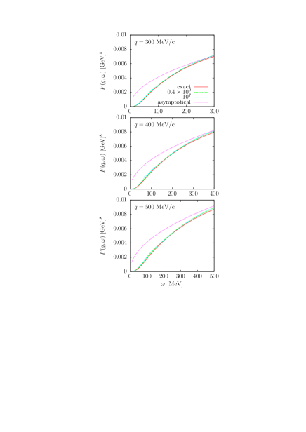
Figure 1: (Color online) Non-relativistic phase-space function calculated for $\omega=300,400,500$ MeV, using a numerical and a semi-analytical approach. The number of points used in two numerical integrations are indicated in the plot. We also show the asymptotic function for comparison.

In Fig. 1 we show the non-relativistic phase-space function $F(q,\omega)$ as a function of $\omega$ for three typical values of the momentum transfer $q=300,400$ and 500 MeV/c. The Fermi momentum is $k_{F}=225$ MeV/c. We compare the two computational methods: the semi-analytical of Eq. (LABEL:fasico2D) and the numerical 7D integration of Eq. (III.2). The semi-analytical result is essentially exact, because we can choose a very small integration step for the 2D integral (using steps of 0.02 or 0.01 the results do not change in the scale of the figure). However the 7D integral is computationally time-consuming and the integration step cannot be very small. Here we compute the integral with a “straightforward” method, as an average over a grid with $n$ total integration points, uniformly distributed. For large $n$ the straightforward integration should give results similar to the Montecarlo methods used in previous calculations Van80 ; DePace03 . The number of points chosen for this calculation was 25 for the variable $\theta^{\prime}_{1}$ (although it can safely be reduced to 16) and 16 for each one of the remaining dimensions. In total the number of points is $n=0.42\times 10^{9}$. This is well above the maximum number $n=10^{6}$–$10^{7}$, typical of previous calculations Van80 ; DePace03 performed using Monte Carlo techniques. Using 10 integration points in each dimension gives very similar results, except for some $\omega$ regions where the numerical error is manifested in an apparently slightly less smooth behavior. Increasing the number of points would improve the results; however, this is not practical because the inclusion of the two-body current would make the calculation too slow. The semi-analytical and numerical results are quite similar, the difference between them being of a few percent. For comparison we also show the asymptotic limit $\omega\rightarrow\infty$, computed using the analytical expression in Eq. (37), which is proportional to $\sqrt{\omega}$. We see that for high $\omega$ the function $F(q,\omega)$ becomes close to the asymptotic value $F_{a}(q,\omega)$. For $q=300$ MeV/c the asymptotic value is almost reached at the photon point $\omega=q$. When $q$ increases, so does the distance to the asymptote at the photon point.

IV Relativistic 2p-2h phase-space

Having two independent calculations of the phase-space function $F(q,\omega)$ in the non-relativistic limit, we now consider the case of the fully relativistic calculation as given by Eq. (LABEL:phase). This involves adding the Lorentz-contraction $m_{N}/E$ factors and using relativistic kinematics in the energy $\delta$-function. Following the scheme of the previous section, again azimuthal symmetry allows one to fix $\phi^{\prime}=0$ and multiply by $2\pi$. To integrate over $p^{\prime}_{1}$ we change to the variable

$$E^{\prime}=E^{\prime}_{1}+E^{\prime}_{2}=\sqrt{p^{\prime}_{1}{}^{2}+m_{N}^{2}}+\sqrt{({\bf p}^{\prime}-{\bf p}^{\prime}_{1})^{2}+m_{N}^{2}}\,,$$ (38)

where again ${\bf p}^{\prime}={\bf h}_{1}+{\bf h}_{2}+{\bf q}$ is the final momentum for a fixed pair of holes. By differentiation we arrive at the following Jacobian:

$$\left|\frac{dp^{\prime}_{1}}{dE^{\prime}}\right|=\left|\frac{p^{\prime}_{1}}{E^{\prime}_{1}}-\frac{{\bf p}^{\prime}_{2}\cdot\widehat{\bf p}^{\prime}_{1}}{E^{\prime}_{2}}\right|^{-1}\,.$$ (39)

The non-relativistic Jacobian of Eq. (26) is recovered for low energies $E^{\prime}_{1}\simeq E^{\prime}_{2}\simeq m_{N}$. As before, integration over $E^{\prime}$ gives $E^{\prime}=E_{1}+E_{2}+\omega$ and the phase-space function becomes

$$F(q,\omega) = 2\pi\int d^{3}h_{1}d^{3}h_{2}d\theta^{\prime}_{1}\sin\theta^{\prime}_{1}\frac{m_{N}^{4}}{E_{1}E_{2}}$$

$$\times \sum_{\alpha=\pm}\left.\frac{p^{\prime}_{1}{}^{2}}{\left|\frac{p^{\prime}_{1}}{E^{\prime}_{1}}-\frac{{\bf p}^{\prime}_{2}\cdot\widehat{\bf p}^{\prime}_{1}}{E^{\prime}_{2}}\right|}\frac{\Theta(p^{\prime}_{1},p^{\prime}_{2},h_{1},h_{2})}{E^{\prime}_{1}E^{\prime}_{2}}\right|_{p^{\prime}_{1}=p^{\prime}_{1}{}^{(\alpha)}}\,,$$

where again the sum inside the integral runs over the two solutions $p^{\prime}_{1}{}^{(\pm)}$ of the energy conservation equation

$$p^{\prime}_{1}{}^{(\pm)}=\frac{1}{\tilde{b}}\left[\tilde{a}\tilde{v}\pm\sqrt{\tilde{a}^{2}-\tilde{b}m_{N}^{2}}\right]\,.$$ (41)

The definitions of the quantities $\tilde{a},\tilde{b},\tilde{v}$ are given in the Appendix. Note that there is a difference between our Jacobian in Eq. (IV) and that given in Eqs. (15–17) of Lal12 ).

The relativistic approach is more involved than the non-relativistic one because it requires taking the square twice in the original equation to eliminate the squared roots in the energies. This can introduce spurious solutions for $p^{\prime}_{1}$ depending on the kinematics, that have to be eliminated from the above sum in the numerical procedure. This is not a trivial task and details are provided in the Appendix. The appearance of spurious solutions is a difference between the relativistic and non-relativistic methods. A second one will be discussed below in relation to a divergence of the integrand. Therefore the relativistic calculation is very involved and it cannot be derived by simply extending the non-relativistic code. We devote the rest of this section to explain in detail how to get the fully relativistic answers.

IV.1 Relativistic asymptotic expansion

Although it is not possible to derive a semi-analytical expression for $F(q,\omega)$ as in the non-relativistic case, it is still possible to take the limit $\omega\rightarrow\infty$ and obtain an analytical result. As in the non-relativistic case, we assume $k_{F},q\ll\omega$. If we add the condition $m_{N}\ll\omega$, we can neglect the momenta and energies of the two holes and write

$$E^{\prime}\sim\omega\kern 28.45274pt{\bf p}^{\prime}\sim{\bf q}\,.$$ (42)

We can also compute the quantities with tildes that appear in the solution of the energy conservation (see Appendix), obtaining

$$\tilde{a} \sim \frac{\omega}{2}$$ (43)

$$\tilde{v} \sim \frac{{\bf q}\cdot\widehat{\bf p}^{\prime}_{1}}{2\omega}$$ (44)

$$\tilde{b} \sim 1\,.$$ (45)

Then the discriminant of Eq. (41) becomes

$$\tilde{a}^{2}-\tilde{b}m_{N}^{2}\sim\frac{\omega^{2}}{4}-m_{N}^{2}\sim\frac{\omega^{2}}{4}\,.$$ (46)

Therefore the allowed solution of the energy conservation equation is

$$p^{\prime}_{1}\sim\frac{{\bf q}\cdot\widehat{\bf p}^{\prime}_{1}}{4}+\frac{\omega}{2}\sim\frac{\omega}{2}\,.$$ (47)

Thus in this limit each nucleon carries half the total energy and momentum

$$E^{\prime}_{1}\sim p^{\prime}_{1}\sim E^{\prime}_{2}\sim p^{\prime}_{2}\sim\frac{\omega}{2}\,.$$ (48)

Now the Jacobian, the denominator in Eq. (IV), can be computed as

$$d\equiv\frac{p^{\prime}_{1}}{E^{\prime}_{1}}-\frac{{\bf p}^{\prime}_{2}\cdot\widehat{\bf p}^{\prime}_{1}}{E^{\prime}_{2}}=1-\frac{({\bf p}^{\prime}-{\bf p}^{\prime}_{1})\cdot\widehat{\bf p}^{\prime}_{1}}{E^{\prime}_{2}}\sim 1+\frac{p^{\prime}_{1}}{E^{\prime}_{2}}\sim 2\,.$$ (49)

Collecting Eqs. (47,48,49), the integrand in Eq. (IV) becomes

$$\frac{p^{\prime}_{1}{}^{2}}{d}\frac{m_{N}^{4}}{E_{1}E_{2}E^{\prime}_{1}E^{\prime}_{2}}\sim\frac{\omega^{2}}{8}\frac{m_{N}^{4}}{m_{N}^{2}\omega^{2}/4}=\frac{m_{N}^{2}}{2}\,.$$ (50)

Finally, performing the integral we obtain the following asymptotic expression

$$F(q,\omega)\stackrel{{\scriptstyle\omega\rightarrow\infty}}{{\longrightarrow}}F_{a}(q,\omega)=4\pi\left(\frac{4}{3}\pi k_{F}^{3}\right)^{2}\frac{m^{2}_{N}}{2}.$$ (51)

In contrast with the non-relativistic behavior, that increases monotonically as $\sqrt{\omega}$, the relativistic result (37) goes to a constant. The Lorentz contraction factors $E/m_{N}$ balance the $\omega^{2}$ behavior coming from the phase-space. This analytical result for high $\omega$ will be useful for comparison of the numerical results for high $\omega$.

IV.2 Relativistic straightforward calculation

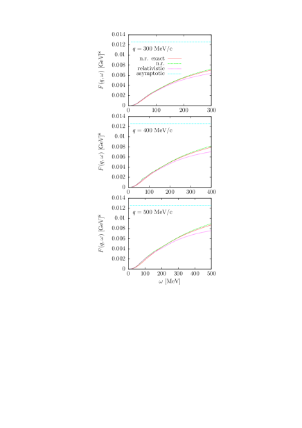
Figure 2: (Color online) Relativistic phase-space function for $q=300,400,500$, calculated using straightforward integration, compared with the non-relativistic calculation using the semi-analytical approach.

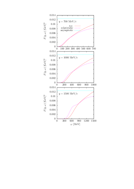
Figure 3: (Color online) Relativistic phase-space function for $q=700,1000,1500$, calculated using straightforward integration compared with the non-relativistic calculation using the semi-analytical approach.

Before going to the high-$q$ region, we first check the relativistic phase-space function results by comparison with the non-relativistic counterpart. Both should agree for low energy. We proceed by performing a straightforward numerical integration of Eq. (IV) as in the non-relativistic case. In Fig. 2 we show the results of this comparison for $q=300,400$ and $500$ MeV/c. We also show both the numerical and “exact” (i.e. using the semi-analytical formula) non-relativistic function $F(q,\omega)$. A uniform distribution with 10 points for each dimension is employed in the 7D integrations. As expected, relativistic and non-relativistic results agree at low energy. The relativistic effects consist of a reduction of the strength at high energy. The amount of this reduction is very small for $q=300$ MeV/c, where the non-relativistic approximation can be safely used, and increases with $q$, reaching about $15\%$ for $q=500$ MeV/c. Thus for low $q$ we agree that a number of $\sim 10^{7}$ points is adequate for numerical integration purposes. In Fig. 5 the asymptotic limit $F_{a}(q,\omega)$ of the relativistic phase-space, Eq. (51), is also shown. For these low $q$ values, $F(q,\omega)$ is still far below the asymptote.

Larger relativistic effects are expected for intermediate to large momentum transfer. In Fig. 3 we display $F(q,\omega)$ for $q=700,1000$ and 1500 MeV/c compared with the exact non-relativistic results. Using straightforward 7D integration we need to increase the number of points to 16 for each dimension in order to reach some stability of the results shown in Fig. 3. However, we find that full convergence would need more points. In fact for $q=700$ MeV/c a small deviation with respect to the exact result can be noticed at low $\omega$. This deviation increases with $q$ and turns into a prominent structure with a “shoulder” shape for $q=1500$ MeV/c. One could be tempted to attribute this effect to relativity. But this is not the case because the same behavior is also present in a non-relativistic numerical calculation. As we will explain below, this is just a consequence of the inadequacy of the straightforward integration method at high $q$. This problem affects only the inner integral over $\theta^{\prime}_{1}$. Below we address this issue by a detailed analysis of the $\theta^{\prime}_{1}$ dependence of the integrand.

V Angular distribution

V.1 Frozen phase-space function

We start fixing a value of $q=3$ GeV/c that is high enough to amplify the misbehavior found above, and also allows to simplify the analysis that follows. In fact we note that for very high $q\gg k_{F}$ all of the hole momenta ${\bf h}_{1}$, ${\bf h}_{2}$ could safely be neglected inside the integral as a first approximation. Since this implies that the initial particles are at rest, we denote this limit the “frozen nucleon approximation“. In particular, the energies of the holes can be substituted by the nucleon mass in the $\delta$ function:

$$F(q,\omega) \sim \int d^{3}h_{1}d^{3}h_{2}d^{3}p^{\prime}_{1}\delta(E^{\prime}_{1}+E^{\prime}_{2}-\omega-2m_{N})$$ (52)

$$\times\Theta(p^{\prime}_{1},p^{\prime}_{2},0,0)\frac{m_{N}^{2}}{E^{\prime}_{1}E^{\prime}_{2}}\,,$$

where ${\bf p}^{\prime}_{2}={\bf q}-{\bf p}^{\prime}_{1}$. Because the integrand does not depend on the hole momenta, one can directly integrate out those variables

$$F(q,\omega) \sim \left(\frac{4}{3}\pi k_{F}^{3}\right)^{2}\int d^{3}p^{\prime}_{1}\delta(E^{\prime}_{1}+E^{\prime}_{2}-\omega-2m_{N})$$ (53)

$$\times\Theta(p^{\prime}_{1},p^{\prime}_{2},0,0)\frac{m_{N}^{2}}{E^{\prime}_{1}E^{\prime}_{2}}\,.$$

Now the integral over $p^{\prime}_{1}$ can be done analytically as before using the delta function, with the same Jacobian evaluated for $h_{1}=h_{2}=0$. The integral over $\phi^{\prime}_{1}$ gives again a factor $2\pi$.

$$F(q,\omega) \sim 2\pi m_{N}^{2}\left(\frac{4}{3}\pi k_{F}^{3}\right)^{2}\int d\theta^{\prime}_{1}\sin\theta^{\prime}_{1}$$

$$\times \sum_{\alpha=\pm}\left.\frac{p^{\prime}_{1}{}^{2}}{\left|\frac{p^{\prime}_{1}}{E^{\prime}_{1}}-\frac{{\bf p}^{\prime}_{2}\cdot\widehat{\bf p}^{\prime}_{1}}{E^{\prime}_{2}}\right|}\frac{\Theta(p^{\prime}_{1},p^{\prime}_{2},0,0)}{E^{\prime}_{1}E^{\prime}_{2}}\right|_{p^{\prime}_{1}=p^{\prime}_{1}{}^{(\alpha)}}\,.$$

Thus in this approximation, the phase-space function is reduced to a one-dimensional integral over the emission angle $\theta^{\prime}_{1}$, which has to be performed numerically.

The frozen nucleon approximation represents just a particular case of the mean-value theorem for the integral over ${\bf h}_{1},{\bf h}_{2}$. We denote with a bar the quantities computed by the mean-value theorem. Thus we define the barred phase-space function

$$\overline{F}(q,\omega) = \left(\frac{4}{3}\pi k_{F}^{3}\right)^{2}\int d^{3}p^{\prime}_{1}\delta(E^{\prime}_{1}+E^{\prime}_{2}-\omega-E_{1}-E_{2})$$ (55)

$$\times\Theta(p^{\prime}_{1},p^{\prime}_{2},h_{1},h_{2})\frac{m_{N}^{4}}{E_{1}E_{2}E^{\prime}_{1}E^{\prime}_{2}}\,,$$

where ${\bf p}^{\prime}_{2}={\bf h}_{1}+{\bf h}_{2}+{\bf q}-{\bf p}^{\prime}_{1}$, and (${\bf h}_{1},{\bf h}_{2})$ are a pair of fixed momenta below the Fermi sea. Going further, we will later turn to the question of how to choose the average nucleon momenta ${\bf h}_{1},{\bf h}_{2}$ for low $q$. For high $q$ we expect this function not to depend too much on the chosen values. So at this point we restrict our study to $\overline{F}(q,\omega)$ in the frozen nucleon approximation, i.e., for $h_{1}=h_{2}=0$.

V.2 Numerical analysis

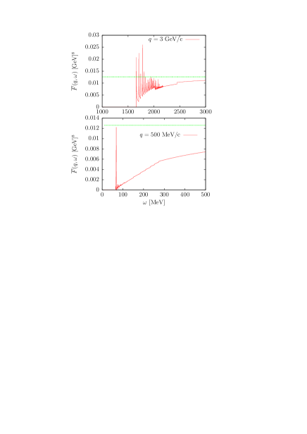
Figure 4: (Color online) Phase-space function for $q=3$ and 0.5 GeV/c, computed using the frozen nucleon approximation for fixed hole momenta $h_{1}=h_{2}=0$, using 100 integration points in emission angle.

We have computed $\overline{F}(q,\omega)$ in the frozen nucleon approximation using 100 points to perform the numerical integral over the emission angle $\theta^{\prime}_{1}$. Results are shown in Fig. 4. A misbehavior due to numerical error is now evident.

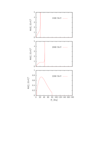
Figure 5: (Color online) Angular dependent phase-space function for $q=3$ GeV/c, for fixed hole momenta $h_{1}=h_{2}=0$, computed for three values of $\omega$ below the quasielastic peak, as a function of the emission angle $\theta^{\prime}_{1}$.

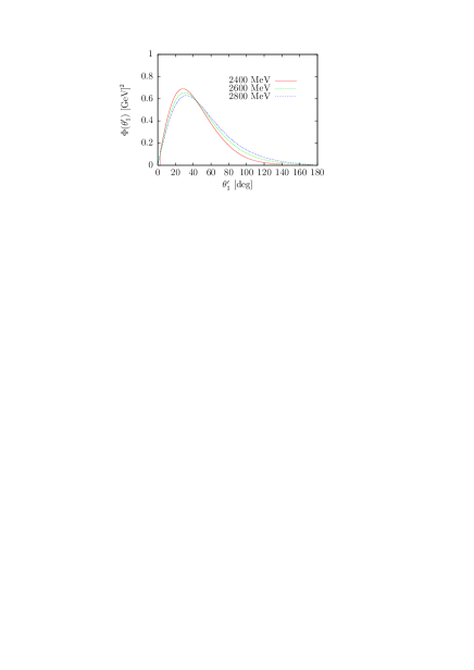
Figure 6: (Color online) Angular dependent phase-space function for $q=3$ GeV/c, for fixed hole momenta $h_{1}=h_{2}=0$, computed for three values of $\omega$ above the quasielastic peak, as a function of the emission angle $\theta^{\prime}_{1}$.

The reason for the appearance of discontinuities by numerical integration becomes apparent by examining the angular dependence of the integrand. We define the angular distribution function, for fixed values of $(q,\omega)$ and ${\bf h}_{1},{\bf h}_{2}$, as

$$\Phi(\theta^{\prime}_{1}) = \sin\theta^{\prime}_{1}\int p^{\prime}_{1}{}^{2}dp^{\prime}_{1}\delta(E_{1}+E_{2}+\omega-E^{\prime}_{1}-E^{\prime}_{2})$$ (56)

$$\times\Theta(p^{\prime}_{1},p^{\prime}_{2},h_{1},h_{2})\frac{m_{N}^{4}}{E_{1}E_{2}E^{\prime}_{1}E^{\prime}_{2}}\,,$$

$$= \sum_{\alpha=\pm}\left.\frac{m_{N}^{4}\sin\theta^{\prime}_{1}p^{\prime}_{1}{}^{2}\Theta(p^{\prime}_{1},p^{\prime}_{2},h_{1},h_{2})}{E_{1}E_{2}E^{\prime}_{1}E^{\prime}_{2}\left|\frac{p^{\prime}_{1}}{E^{\prime}_{1}}-\frac{{\bf p}^{\prime}_{2}\cdot\widehat{\bf p}^{\prime}_{1}}{E^{\prime}_{2}}\right|}\right|_{p^{\prime}_{1}=p^{\prime}_{1}{}^{(\alpha)}}$$

where once more ${\bf p}^{\prime}_{2}={\bf h}_{1}+{\bf h}_{2}+{\bf q}-{\bf p}^{\prime}_{1}$, such that the phase-space function is obtained by integration over the emission angle $\theta^{\prime}_{1}$

$$\overline{F}(q,\omega)=\left(\frac{4}{3}\pi k_{F}^{3}\right)^{2}2\pi\int_{0}^{\pi}d\theta^{\prime}_{1}\Phi(\theta^{\prime}_{1})\,.$$ (57)

The function $\Phi(\theta^{\prime}_{1})$ thus measures the distribution of final nucleons as a function of the angle $\theta^{\prime}_{1}$. This function is computed analytically, given by the integrand in Eq. (V.1).

Results for $\Phi(\theta^{\prime}_{1})$ are shown in Fig. 5 for $h_{1}=h_{2}=0$, $q=3$ GeV/c and for three values of $\omega=1800$, 2000 and 2200 MeV. For low $\omega$, the function $\Phi(\theta^{\prime}_{1})$ is different from zero in a narrow angular interval at low angles. At the upper limit of the interval a divergence appears as a thin peak which is infinitely high due to a zero in the denominator. The angular interval increases with $\omega$ as does the value of the divergent angle. For $\omega=2200$ MeV there is no divergence because Pauli blocking forbids reaching the divergent angle. Instead the angular distribution starts and ends abruptly due to the discontinuity produced by the step functions. Note that the values of $\omega$ shown in Fig. 5 are located below the quasielastic (QE) peak, that is defined by

$$\omega=\sqrt{m_{N}^{2}+q^{2}}-m_{N}\,.$$ (58)

For $q=3$ GeV/c, the QE peak is located roughly at $\omega=2200$ MeV.

The situation is different for $\omega$ values above the QE peak. In Fig. 6 we show in the same plot the angular distribution for $\omega=2400$, 2600 and 2800 MeV. The angular distribution is smooth and similar in the three cases, with a tail that goes smoothly to zero for high angles. Increasing the energy just extends the angular tail of $\Phi(\theta^{\prime}_{1})$ farther and slightly decreases its strength for low angles, while its maximum is shifted a few degrees to the right. Note that the maximum of the angular distribution for these high energies is located around 30 degrees.

Thus the origin of the discontinuities observed in Fig. 4 is because the angular distribution $\Phi(\theta^{\prime}_{1})$ has a divergence or pole for some angle, resulting in a thin peak close to the pole. When one tries to compute the integral in Eq. (57) numerically, by evaluating the integrand at some discrete set of $\theta^{\prime}_{1}$ points, sometimes a value close to the pole is reached, producing the apparent discontinuity. Trying to integrate the peak numerically is hard because it is very narrow; so even with many thousands of points there are still numerical errors.

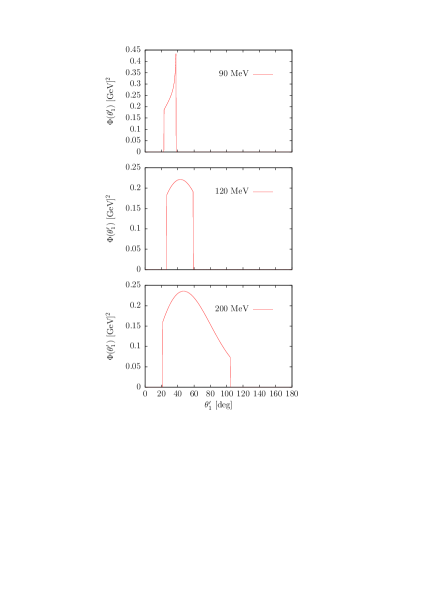
Figure 7: (Color online) Angular dependent phase-space function for $q=500$ MeV/c, for fixed hole momenta $h_{1}=h_{2}=0$, computed for three values of $\omega$ around the quasielastic peak as a function of the emission angle $\theta^{\prime}_{1}$.

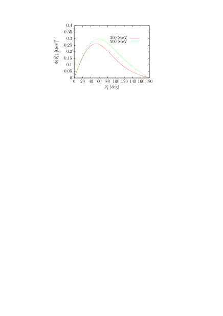
Figure 8: (Color online) Angular dependent phase-space function for $q=500$ MeV/c, for fixed hole momenta $h_{1}=h_{2}=0$, computed for $\omega=300$ and 500 MeV as a function of the emission angle $\theta^{\prime}_{1}$.

Up to now we have analyzed the problem of the singularity of the angular distribution for high momentum. Now the question that arises is why this problem did not apparently emerge when we discussed the non-relativistic case, that is, for low momentum transfer. The real fact is that this singularity also appears for low $q$, but only for very low energy transfer (due to kinematical reasons). We can see this in the lower panel of Fig. 4, where we display the function $\overline{F}(q,\omega)$ in the frozen nucleon approximation for $q=500$ MeV/c. As before we use 100 integration points. There is a narrow peak at threshold followed by rapid, small oscillations. In Fig. 7 we show the corresponding angular distribution for several values of $\omega$. For $\omega=90$ MeV we again see a peak corresponding to a singularity at the endpoint, but the peak is not as narrow as for high $q$. Therefore, it can be integrated with few points. Only for very small $\omega\sim 66$ MeV (not shown in the figure), we find a very narrow peak. For higher values of $\omega$ there is no singularity and the angular distribution is smooth and wide enough to obtain reasonable results with few integration points. At the QE peak, $\omega\sim 120$ MeV, the angular distribution is zero outside the interval $25^{\circ}<\theta^{\prime}_{1}<60^{\circ}$ due to Pauli blocking, that is also present for $\omega=200$ MeV. For larger values of $\omega$ (see Fig. 8), there is no Pauli blocking and $\Phi(\theta^{\prime}_{1})$ is a smooth distribution with a maximum that slightly increases with $\omega$ and shifts towards higher angles.

V.3 Kinematical analysis

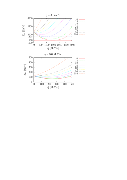
Figure 9: (Color online) Plot of the excitation energy of a pair of nucleons at rest for two values of the momentum transfer and for several emission angles, as a function of the emission momentum $p^{\prime}_{1}$.

We have seen that the angular distribution presents singularities for some emission angles. The occurrence of the singularity is a consequence of the kinematical dependence of the excitation energy of the 2p-2h states

$$E_{ex}=E^{\prime}_{1}+E^{\prime}_{2}-E_{1}-E_{2}.$$ (59)

In the frozen nucleon limit, it is given by

$$E_{ex}=\sqrt{p^{\prime}_{1}{}^{2}+m_{N}^{2}}+\sqrt{p^{\prime}_{1}{}^{2}+m_{N}^{2}+q^{2}-2p^{\prime}_{1}q\cos\theta^{\prime}_{1}}-2m_{N}\,,$$ (60)

which depends on the variables $q,p^{\prime}_{1}$ and $\theta^{\prime}_{1}$. In Fig. 9 we show the value of the excitation energy as a function of the emission momentum, for large and intermediate values of $q$. For each $q$ we plot curves for several values of the emission angle $\theta^{\prime}_{1}$ from 0 to 180^∘.

In the upper panel the momentum transfer is $q=3$ GeV/c. For $p^{\prime}_{1}=0$ all of the curves collapse to the quasielastic peak energy. The lower horizontal straight line corresponds to energy $\omega=1660$ MeV, and this is the minimum energy for which two-particle emission is possible by energy-momentum conservation, that is, there is a solution of the equation $\omega=E_{ex}(p^{\prime}_{1})$ that corresponds to the intersection point between the straight line and the lower excitation-energy curve for $\theta^{\prime}_{1}=0$, corresponding precisely to the minimum of the curve. For angles above $\theta^{\prime}_{1}=0$ two-particle emission is not possible with this excitation energy. This explains why for very low energy the emission is forward.

If we increase the excitation energy to $\omega=1875$ MeV, represented by the upper straight line of Fig. 9, we see that it crosses all of the curves below $\theta^{\prime}_{1}=30^{\circ}$, that is, emission is possible only for angles in the interval $[0,30^{\circ}]$. We also see that for each angle in this interval there are two values of $p^{\prime}_{1}$ with this excitation energy, corresponding to the two solutions $p^{\prime}_{1}{}^{(\pm)}$, Eq. (41), of the energy conservation equation $\omega=E_{ex}$.

For $30^{\circ}$ both solutions coincide with the position of the minimum of $E_{ex}(p^{\prime}_{1})$. A singularity of the angular distribution $\Phi(\theta^{\prime}_{1})$ is expected at the end angle $\theta^{\prime}_{1}=30^{\circ}$, because the minimum of the curve $E_{ex}(p^{\prime}_{1})$ holds precisely at the solution of the energy conservation equation. Thus

$$\frac{dE_{ex}}{dp^{\prime}_{1}}=0.$$ (61)

Now the angular distribution is proportional to

$$\int dp^{\prime}_{1}p^{\prime}_{1}{}^{2}\delta(E_{ex}-\omega),$$ (62)

which may be computed by changing variables $p^{\prime}_{1}\rightarrow E_{ex}(p^{\prime}_{1})$. Therefore, it is proportional to the Jacobian

$$dp^{\prime}_{1}=\frac{dE_{ex}}{\left|\frac{dE_{ex}}{dp^{\prime}_{1}}\right|}\,,$$ (63)

that diverges at the minimum because the denominator is zero. Note from Fig. 9 that this divergence of the angular distribution occurs for all the $\omega$ values below the QE peak, but at a different value of the angle. This angle must be such that the corresponding excitation energy curve in Fig. 9 has its minimum at $E_{ex}=\omega$.

Above the quasielastic peak energy $\omega_{QE}$ there is no divergence because, from Fig. 9, the minimum is always below $\omega_{QE}$. We also see that above $90^{\circ}$ there are no minima, so divergences only occur for angles below $90^{\circ}$. This can also be seen in Eq. (60): for $\cos\theta^{\prime}_{1}<0$ the excitation energy increases with $p^{\prime}_{1}$.

The same conclusions can be drawn for low momentum transfer. From the lower panel of Fig. 9 all of the excitation energy curves for $q=500$ MeV/c have a minimum below $90^{\circ}$. The main difference with respect to the high $q$ case is that the quasielastic peak occurs at very low $\omega$ compared with $q$ and that the minimum $p^{\prime}_{1}$ for large angles is located below $k_{F}$, and does not contribute to the angular distribution due to Pauli blocking. Therefore, there will be singularities only for very low $\omega$ values.

For smaller values of $q\leq 500$ MeV/c the minima are always below $k_{F}$ and there are no singularities in the angular distribution.

Thus the singularity problem appears only for intermediate to high $q$. It could seem that the divergence in the angular distribution could be observed in a coincidence experiment by fixing the emission angle and energy transfer at the position of a divergence. However, this cannot be the case because our discussion is valid only in the frozen nucleon approximation where the initial nucleons are at rest. In a real system an integration over initial momenta is implied, removing the singularity.

VI Theoretical analysis of the angular distribution

VI.1 Allowed angular intervals and divergences

Our next goal is first to find analytically the angle $\theta^{\prime}_{1}$ where the angular distribution diverges as well as the kind of singularity (we shall see that the singularity is integrable, as it should be by the definition of the phase-space function), and second to design a method to compute the angular integral in the vicinity of the singular point.

We start with the formula for the denominator in the angular distribution, given by the Jacobian, Eq. (39). Using momentum conservation ${\bf p}^{\prime}_{2}={\bf p}^{\prime}-{\bf p}^{\prime}_{1}$ it can be written in the form:

$$d\equiv\frac{p^{\prime}_{1}}{E^{\prime}_{1}}-\frac{{\bf p}^{\prime}_{2}\cdot\widehat{\bf p}^{\prime}_{1}}{E^{\prime}_{2}}=\frac{E^{\prime}}{E^{\prime}_{1}E^{\prime}_{2}}\left(p^{\prime}_{1}-\tilde{v}E^{\prime}_{1}\right)\,,$$ (64)

where $\tilde{v}$ is defined in the Appendix, Eq. (109). Using energy conservation, written in the equivalent form (see Eq. (107) in the Appendix), $E^{\prime}_{1}=\tilde{a}+\tilde{v}p^{\prime}_{1}$, we arrive at

$$d=\frac{E^{\prime}}{E^{\prime}_{1}E^{\prime}_{2}}\left(\tilde{b}p^{\prime}_{1}-\tilde{v}\tilde{a}\right)\,,$$ (65)

where $\tilde{b}$ and $\tilde{a}$ have been defined in the Appendix, Eqs. (111,108). The quantity in brackets is the discriminant in the solution of the second-order equation for the momentum $p^{\prime}_{1}$ given in Eq. (41). Therefore we obtain

$$d=\pm\frac{E^{\prime}}{E^{\prime}_{1}E^{\prime}_{2}}\sqrt{D}\,,$$ (66)

where the relativistic discriminant is defined as

$$D=\tilde{a}^{2}-\tilde{b}m_{N}^{2}\,.$$ (67)

Using $\tilde{b}=1-\tilde{v}^{2}$, this can be expressed equivalently as

$$D=m_{N}^{2}\left(\tilde{v}^{2}-\frac{m_{N}^{2}-\tilde{a}^{2}}{m_{N}^{2}}\right)\,.$$ (68)

To make explicit the dependence on the emission angle $\theta^{\prime}_{1}$, implicit in the variable $\tilde{v}={\bf p}^{\prime}\cdot\widehat{\bf p}^{\prime}_{1}/E^{\prime}$, we note that the vector $\widehat{\bf p}^{\prime}_{1}$ has Cartesian coordinates

$$\widehat{\bf p}^{\prime}_{1}=(\sin\theta^{\prime}_{1},0,\cos\theta^{\prime}_{1})\,.$$ (69)

We recall that we are using the reference system where ${\bf q}$ is in the $z$-axis and that we are taking $\phi^{\prime}_{1}=0$. Therefore $\widehat{\bf p}^{\prime}_{1}$ is contained in the scattering plane, $xz$.

The scalar product appearing in $\tilde{v}$ is

$${\bf p}^{\prime}\cdot\widehat{\bf p}^{\prime}_{1}=p^{\prime}_{x}\sin\theta^{\prime}_{1}+p^{\prime}_{2}\cos\theta^{\prime}_{1}\,.$$ (70)

We now define the final momentum vector projected over the scattering plane

$${\bf s}^{\prime}=(p^{\prime}_{x},0,p^{\prime}_{z})=s^{\prime}(\sin\alpha,0,\cos\alpha)\,.$$ (71)

This equation defines $\alpha$ as the angle between ${\bf s}^{\prime}$ and ${\bf q}$. With this definition, the scalar product can be written

$${\bf p}^{\prime}\cdot\widehat{\bf p}^{\prime}_{1}=s^{\prime}\cos(\theta^{\prime}_{1}-\alpha)\,.$$ (72)

Now the discriminant $D$ can be easily written in terms of the vector ${\bf s}^{\prime}$ as

$$D=\frac{m_{N}^{2}s^{\prime}{}^{2}}{E^{\prime}{}^{2}}\left[\cos^{2}(\theta^{\prime}_{1}-\alpha)-w_{0}\right]\,,$$ (73)

where we have defined the non-dimensional variable

$$w_{0}=\frac{E^{\prime}{}^{2}}{s^{\prime}{}^{2}}\left(1-\frac{\tilde{a}^{2}}{m_{N}^{2}}\right)\,.$$ (74)

This development allows one to write the integral over emission angle $\theta^{\prime}_{1}$ appearing in Eq. (IV), for fixed ${\bf h}_{1},{\bf h}_{2}$, as

$$I \equiv \int_{0}^{\pi}d\theta^{\prime}_{1}\sin\theta^{\prime}_{1}\frac{p^{\prime}_{1}{}^{2}}{|d|}\frac{m_{N}^{4}}{E_{1}E_{2}E^{\prime}_{1}E^{\prime}_{2}}\Theta(p^{\prime}_{1},p^{\prime}_{2},h_{1},h_{2})$$ (75)

$$= \int_{0}^{\pi}d\theta^{\prime}_{1}\sin\theta^{\prime}_{1}\frac{m_{N}^{4}}{E_{1}E_{2}E^{\prime}_{1}E^{\prime}_{2}}\Theta(p^{\prime}_{1},p^{\prime}_{2},h_{1},h_{2})$$

$$\times \frac{\left(\tilde{a}\tilde{v}\pm\sqrt{D}\right)^{2}\theta(D)}{\frac{\tilde{b}^{2}}{E^{\prime}_{1}E^{\prime}_{2}}m_{N}s^{\prime}\sqrt{\cos^{2}(\theta^{\prime}_{1}-\alpha)-w_{0}}}\,,$$

where $p^{\prime}_{1}=p^{\prime}_{1}{}^{(\pm)}=(\tilde{a}\tilde{v}\pm\sqrt{D})/\tilde{b}$ is one of the solutions of energy conservation. A sum over the two solutions will be performed later. The explicit step function $\theta(D)$ indicates that there is only a solution of energy conservation for a positive value of $D$, or equivalently, for positive values of the function

$$g(\theta^{\prime}_{1})\equiv\cos^{2}(\theta^{\prime}_{1}-\alpha)-w_{0}.$$ (76)

Thus we have demonstrated that the integral $I$ has the general form

$$I=\int_{0}^{\pi}d\theta^{\prime}_{1}\frac{f(\theta^{\prime}_{1})}{\sqrt{g(\theta^{\prime}_{1})}}\theta(g(\theta^{\prime}_{1}))\,,$$ (77)

where the function $f(\theta)$ in general has no singularities. This function will contain the hadronic current when computing the response functions. The denominator, however, could be zero for some kinematics. We can consider three cases depending on the value of $w_{0}$:

• If $w_{0}>1$ there is no solution of the energy conservation equation,

• If $w_{0}<0$ there is always solution of the energy conservation equation. All of the angles are allowed and there is no singularity in the angular distribution.

• If $0\leq w_{0}\leq 1$ the angular distribution is different from zero only in one or two angular intervals. The angular distribution is infinite for $g(\theta^{\prime}_{1})=0$ or $\cos^{2}(\theta^{\prime}_{1}-\alpha)=w_{0}$.

In the last case there are two solutions for this equation given implicitly by $\cos(\theta^{\prime}_{1}-\alpha)=\pm\sqrt{w_{0}}$. Taking the arc-cosine, we define the two angles

$$\varphi_{1}\equiv\cos^{-1}\sqrt{w_{0}},\kern 28.45274pt\varphi_{2}\equiv\cos^{-1}(-\sqrt{w_{0}}),$$ (78)

such that $0\leq\varphi_{1},\varphi_{2}<\pi$. The position of the divergence is defined up to a $\pm\pi$ term

$$\theta^{\prime}_{1}-\alpha=\varphi_{1}\pm\pi,\varphi_{2}\pm\pi\,.$$ (79)

To determine the exact position of the divergence and the intervals of the allowed angular distribution we must analyze the eight possible cases displayed in Fig. 10. The eight cases are classified according to the values of $\alpha$ and $w_{0}$. They are the following:

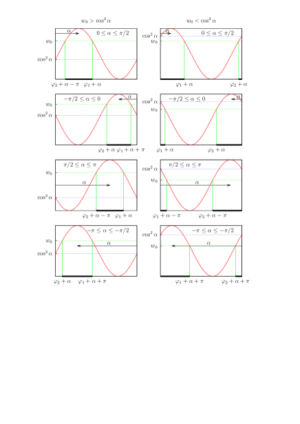
Figure 10: (Color online) Plots of the function $\cos^{2}(\theta^{\prime}_{1}-\alpha)$ as a function of $\theta^{\prime}_{1}$, for the geometries of the 8 different cases depending on the values of $\alpha$ and $w_{0}$. In each panel we show with bold lines the angular intervals where the integral is performed $\cos^{2}(\theta^{\prime}_{1}-\alpha)>w_{0}^{2}$

• Case (1a): $0\leq\alpha\leq\frac{\pi}{2}$ and $w_{0}>\cos^{2}\alpha$. The angular distribution interval is

  $$L\equiv[\varphi_{2}+\alpha-\pi,\varphi_{1}+\alpha]$$ (80)

• Case (1b): $0\leq\alpha\leq\frac{\pi}{2}$ and $w_{0}<\cos^{2}\alpha$. There are two angular distribution intervals

  $$L_{1}\equiv[0,\varphi_{1}+\alpha]\,,\kern 28.45274ptL_{2}\equiv[\varphi_{2}+\alpha,\pi]\,.$$ (81)

• Case (2a): $-\frac{\pi}{2}\leq\alpha\leq 0$ and $w_{0}>\cos^{2}\alpha$. The angular distribution interval is

  $$L\equiv[\varphi_{2}+\alpha,\varphi_{1}+\alpha+\pi]\,.$$ (82)

• Case (2b): $-\frac{\pi}{2}\leq\alpha\leq 0$ and $w_{0}<\cos^{2}\alpha$. There are two angular distribution intervals

  $$L_{1}\equiv[0,\varphi_{1}+\alpha]\,,\kern 28.45274ptL_{2}\equiv[\varphi_{2}+\alpha,\pi]\,.$$ (83)

• Case (3a): $\frac{\pi}{2}\leq\alpha\leq\pi$ and $w_{0}>\cos^{2}\alpha$. The angular distribution interval is

  $$L\equiv[\varphi_{2}+\alpha-\pi,\varphi_{1}+\alpha]\,.$$ (84)

• Case (3b): $\frac{\pi}{2}\leq\alpha\leq\pi$ and $w_{0}<\cos^{2}\alpha$. There are two angular distribution intervals

  $$L_{1}\equiv[0,\varphi_{1}+\alpha-\pi]\,,\kern 28.45274ptL_{2}\equiv[\varphi_{2}+\alpha-\pi,\pi]\,.$$ (85)

• Case (4a): $-\pi\leq\alpha\leq-\frac{\pi}{2}$ and $w_{0}>\cos^{2}\alpha$. The angular distribution interval is

  $$L\equiv[\varphi_{2}+\alpha,\varphi_{1}+\alpha+\pi]\,.$$ (86)

• Case (4b): $-\pi\leq\alpha\leq-\frac{\pi}{2}$ and $w_{0}<\cos^{2}\alpha$. There are two angular distribution intervals

  $$L_{1}\equiv[0,\varphi_{1}+\alpha+\pi]\,,\kern 28.45274ptL_{2}\equiv[\varphi_{2}+\alpha+\pi,\pi]\,.$$ (87)

Note that only the cases 1 and 2 are possible for large $q>2k_{F}$, which is the case of most interest for neutrino and electron scattering applications at intermediate energies. Cases 3 and 4 are only possible for low $q$, where the non relativistic formalism can be applied. They are given here for completeness.

VI.2 Integration of divergences

Two singularities appear in the angular distribution at the boundaries of the allowed intervals, corresponding to $\cos^{2}(\theta^{\prime}_{1}-\alpha)=w_{0}$.

To integrate the resulting function numerically is not simple because the width of the infinite peak is small around the asymptote and a very small step is needed. However the divergence is integrable. The situation is similar to performing the integral of the function $1/\sqrt{x}$ between 0 and $\epsilon>0$

$$\int_{0}^{\epsilon}\frac{dx}{\sqrt{x}}=\left.2\sqrt{x}\right|_{0}^{\epsilon}=2\sqrt{\epsilon}\,.$$ (88)

The integrand is infinite for $x=0$, but the integral is well defined because the function increases slower than $x^{-1}$.

In our case we exploit the above property of the integral of $1/\sqrt{x}$, that is, we perform the integral around the divergence analytically by assuming that the numerator does not change too much in a small interval.

Specifically, we consider the case (1a), where the integration interval $[\theta_{1},\theta_{2}]$ is given in Eq. (80) and there are two singularities at the ends of the interval. We are then involved with an integral of the kind

$$I(\theta_{1},\theta_{2}) \equiv \int_{\theta_{1}}^{\theta_{2}}\frac{f(\theta)d\theta}{\sqrt{g(\theta)}}$$

$$= I(\theta_{1},\theta_{1}+\epsilon)+I(\theta_{1}+\epsilon,\theta_{2}-\epsilon)+I(\theta_{2}-\epsilon,\theta_{2})\,.$$

We have written this equation as the sum of three integrals. Here $\epsilon$ is a small number that will allow us to integrate analytically around the divergence points by exploiting Eq. (88). First we re-write the integrand by multiplying and dividing by the derivative $g^{\prime}(\theta)=dg/d\theta$, as

$$\frac{f(\theta)}{\sqrt{g(\theta)}}=2\frac{f(\theta)}{g^{\prime}(\theta)}\frac{d\sqrt{g(\theta)}}{d\theta}\,.$$ (90)

Under the assumption that the function $\frac{f(\theta)}{g^{\prime}(\theta)}$ is finite and almost constant in the small interval $[\theta_{1},\theta_{1}+\epsilon]$, the integral around the first singular point can be approximated by

$$I(\theta_{1},\theta_{1}+\epsilon) = \int_{\theta_{1}}^{\theta_{1}+\epsilon}\frac{f(\theta)d\theta}{\sqrt{g(\theta)}}$$ (91)

$$\simeq 2\frac{f(\theta_{1})}{g^{\prime}(\theta_{1})}\int_{\theta_{1}}^{\theta_{1}+\epsilon}\frac{d\sqrt{g(\theta)}}{d\theta}d\theta$$

$$= 2\frac{f(\theta_{1})}{g^{\prime}(\theta_{1})}\sqrt{g(\theta_{1}+\epsilon)}$$

because $g(\theta_{1})=0$. This is a result that already can be used in practice to compute the integral around the divergence. However, we prefer to write it in an equivalent way that is valid for the eight cases. Using the fact that $\epsilon$ is small, we first expand $g(\theta_{1}-\epsilon)\simeq-g^{\prime}(\theta_{1})\epsilon$. Therefore

$$I(\theta_{1},\theta_{1}+\epsilon)=\frac{2f(\theta_{1})}{\sqrt{g^{\prime}(\theta_{1})}}\sqrt{\epsilon}\,.$$ (92)

From the definition of $g(\theta)$, Eq. (76),

$$g^{\prime}(\theta)=-2\cos(\theta-\alpha)\sin(\theta-\alpha)$$ (93)

using $\theta_{1}=\varphi_{2}+\alpha-\pi$, and we get the following values at the divergence: $\cos(\theta_{1}-\alpha)=\sqrt{w_{0}}$, and $\sin(\theta_{1}-\alpha)=-\sqrt{1-w_{0}}$. We obtain for the derivative at $\theta_{1}$

$$g^{\prime}(\theta_{1})=2\sqrt{w_{0}(1-w_{0})}\,.$$ (94)

The integral around the singular point $\theta_{1}$ can be finally written as

$$I(\theta_{1},\theta_{1}+\epsilon)=\frac{f(\theta_{1})\sqrt{2\epsilon}}{[w_{0}(1-w_{0})]^{1/4}}\,.$$ (95)

A similar calculation gives for the integral around the upper divergence angle $\theta_{2}$ the result:

$$I(\theta_{2}-\epsilon,\theta_{2})\simeq-\frac{2f(\theta_{2})}{g^{\prime}(\theta_{2})}\sqrt{g(\theta_{2}-\epsilon)}\simeq\frac{f(\theta_{2})\sqrt{2\epsilon}}{[w_{0}(1-w_{0})]^{1/4}}\,.$$ (96)

Finally, we can write the integral as

$$I(\theta_{1},\theta_{2})=I(\theta_{1}+\epsilon,\theta_{2}-\epsilon)+\frac{[f(\theta_{1})+f(\theta_{2})]\sqrt{2\epsilon}}{[w_{0}(1-w_{0})]^{1/4}}\,.$$ (97)

The integral $I(\theta_{1}+\epsilon,\theta_{2}-\epsilon)$ can now be evaluated numerically.

A systematic analysis of the eight cases (a1)–(4b) shows that this result can be extended for all kinematics. That is, the contribution from the neighborhood of a singularity $\theta_{1}$ is given by Eq. (95), where $\epsilon$ is a small integration interval to the left or to the right of the divergence point.

VII Results for the 2p-2h phase-space function

Here we present results for $F(q,\omega)$ using the integration method introduced in the previous section. It results in the following integration algorithm: For each pair of holes ${\bf h}_{1},{\bf h}_{2}$ we first compute the variable $w_{0}$, Eq. (74). According to the previous section, if $w_{0}>1$, there is no solution of the energy conservation equation and consequently, this pair of holes does not contribute to $F(q,\omega)$. If $w_{0}<0$, all of the emission angles are allowed for the first particle, so we can safely compute the integral over $\theta^{\prime}_{1}$ numerically in the interval $[0,\pi]$. If $0\leq w_{0}\leq 1$ then we compute the angle $\alpha$ defined in Eq. (71) and determine the case (1a)–(4b) to which these kinematics belong, and the corresponding allowed intervals, Eqs. (80–87). We integrate numerically within each one of the allowed intervals, up to a distance $\epsilon$ to the singular point. The integral around the singular point is made using the semi-analytical method discussed in the previous section. Each singular point contributes with a term given by Eq. (95) which we add to the numerical integral. We use the value $\epsilon=0.01$, but we have checked that the results do not depend on $\epsilon$. For the numerical integrals we use Simpson method.

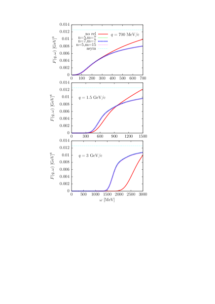
Figure 11: (Color online) Total phase-space function for three values of the momentum transfer. The number of integration points in each dimension in the hole variables is indicated by $n$. The number of integration points over the emission angle $\theta^{\prime}_{1}$ is indicated as $m$. We also show the non-relativistic, exact result and the relativistic asymptotic value.

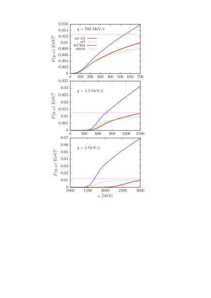
Figure 12: (Color online) Effect of implementing relativistic kinematics in a non-relativistic calculation of $F(q,\omega)$. Solid lines: non-relativistic result. Thick dotted lines: relativistic kinematics only without the relativistic factors $m_{N}/E$. Thin dashed lines: fully relativistic result.

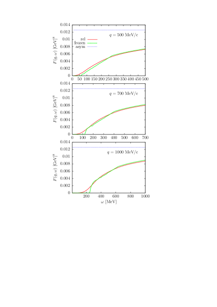
Figure 13: (Color online) Relativistic phase-space function $F(q,\omega)$ compared with the frozen nucleon approximation for low to intermediate momentum transfer.

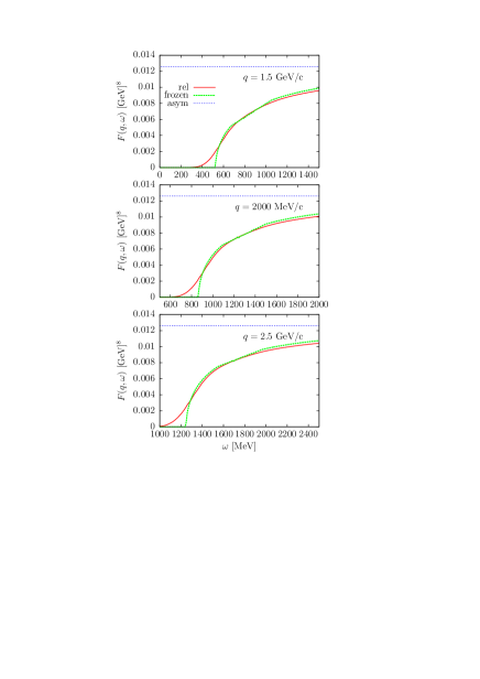
Figure 14: (Color online) Relativistic phase-space function $F(q,\omega)$ compared with the frozen nucleon approximation for high momentum transfer.

In Fig. 11 we show the total phase-space function $F(q,\omega)$ for three values of the momentum transfer, $q=700$, 1500 and 3000 MeV/c. We study the convergence of the 7D integral. For the integral over the two holes ${\bf h}_{1},{\bf h}_{2}$, we show results for $n=5$ and 7 points for each dimension. For the inner integral over the emission angle we use $m=7$ and 15 points. We see that using $(n,m)=(5,7)$ there is almost no difference with the other cases $(7,7)$ and $(5,15)$. As we have seen, the new algorithm allows us to compute with small error the inner integral over $\theta^{\prime}_{1}$ using only 7 points. The dependence on the hole momenta, ${\bf h}_{1},{\bf h}_{2}$, of the resulting function is very smooth and can be safely computed with a small number of integration points. The fact that very precise results can be obtained using $(n,m)=(5,7)$ is an important improvement over previous approaches, taking into account that the total number of points is $5^{6}\times 7\simeq 10^{5}$, that is, two orders of magnitude less than $10^{7}$ (10 points for each dimension). Thus the computational time when we include the nuclear current matrix elements will be considerably reduced.

In Fig. 11 we also show the non-relativistic, exact result, computed using the semi-analytical expression, Eq. (LABEL:fasico2D). For $q=700$ MeV/c both relativistic and non-relativistic results coincide for low energy $\omega<300$ MeV. Above this energy the relativistic result is below the non-relativistic one. For $q=1.5$ GeV/c there are clear differences between the two results for all energies. For high momentum transfer $q=3$ GeV/c, they are completely different. The non-relativistic function is pushed toward higher energies due to the quadratic momentum dependence of the non-relativistic kinetic energy. Thus for $q=1.5$ GeV/c, the relativistic results are above (below) the non-relativistic ones for low (high) energy. For $q=3$ GeV/c the relativistic results are above for all $\omega$ values allowed.

In all cases $F(q,\omega)$ is below the asymptotic value, Eq. (51), also shown in Fig. 11.

In Fig. 12 we get a deeper insight into the size of relativistic effects. There we show results for $F(q,\omega)$ computed using relativistic kinematics only, but without including the relativistic Lorentz-contraction factors $m_{N}/E$ in particles and holes. The results increase a lot with respect to the non-relativistic ones. This is related to the fact pointed out after Eq. (51) for the asymptotic limit of the relativistic phase-space integral. Without the Lorentz factors, the function $F(q,\omega)$ would increase as $\omega^{2}$. This seems to indicate that in order to “relativize” a non-relativistic 2p-2h model, implementing only relativistic kinematics is not sufficient, since it goes in the wrong direction. In fact, results in Fig. 12 show that the effects coming solely from the relativistic kinematics lead to differences even larger than the discrepancy between the non-relativistic and the fully relativistic calculations. Therefore, it is essential also to include the Lorentz factors $m_{N}/E$.

Note that the behaviour of relativistic effects in the 1p-1h channel goes in the opposite direction to the one discussed here in the 2p-2h channel. In fact, in Ama02 it was shown that implementing relativistic kinematics without the $m_{N}/E$ factors in the non relativistic 1p-1h response function, gives a result closer to the exact relativistic response function (see Fig. 33 of Ama02 ).

In Figs. 13 and 14 we present the results of a study of the validity of the frozen nucleon approximation to compute $F(q,\omega)$ in a range of momentum transfers. This approximation was introduced for high momentum transfer $q=3$ GeV/c, neglecting the momenta of the two holes inside the 7D integral, thus reducing it to a 1D integral over the emission angle $\theta^{\prime}_{1}$. In Fig. 14 the momentum transfer is still high and the frozen nucleon approximation remains valid. In Fig. 13 the values of $q$ are not so large, and one could think that the frozen nucleon approximation is not valid. However, the results of Fig. 13 demonstrate that it is still a good approximation for moderate momentum transfer except for very low energy transfer, where the function $F(q,\omega)$ is small. This is a promising result: if the frozen nucleon approximation could be extended to the full response functions when including the nuclear current, this would mean that the 2p-2h cross section could be approximated by 1D integrals over the emission angle which would be easy and fast to compute. In particular, calculations of this kind could be implemented in existing Monte-Carlo codes.

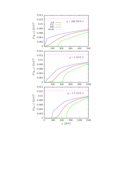
Figure 15: (Color online) Relativistic phase-space function $F(q,\omega)$ compared with the average-momentum approximation $\overline{F}(q,\omega)$ for a pair of nucleons with momentum $200$ MeV/c. In the UU configuration, both nucleons move along ${\bf q}$ (up). In the DD configuration, both move opposite to ${\bf q}$ (down).

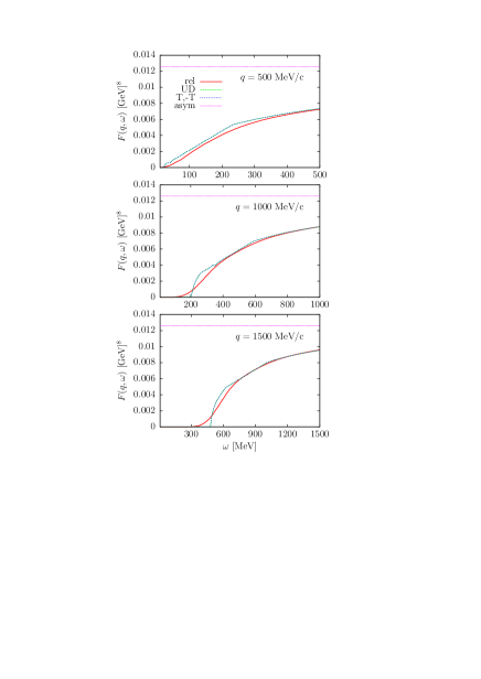
Figure 16: (Color online) Relativistic phase-space function $F(q,\omega)$ compared with the average-momentum approximation $\overline{F}(q,\omega)$ for a pair of nucleons with momentum $200$ MeV/c pointing in opposite directions (total momentum equal to zero). In the UD configuration one moves along ${\bf q}$ (U) and the other opposite to ${\bf q}$ (D). In the T,-T configuration one moves in the $x$-direction and the other in the $-x$-direction.

Figure 17: (Color online) Relativistic phase-space function $F(q,\omega)$ compared with the average-momentum approximation $\overline{F}(q,\omega)$ for a pair of nucleons with momentum $200$ MeV/c pointing in perpendicular directions. In the T,T’ configuration one moves along $x$ (T) and the other along to $y$ (T’). In the -T,-T’ configuration they move along the $-x$ and $-y$ directions, respectively.

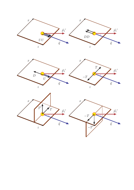
Figure 18: (Color online) Geometry employed for emission of a pair of nucleons with momenta parallel (cases $UU$, $DD$), anti-parallel (cases $UD$, $T-T$) and perpendicular (cases $TT^{\prime}$, $-T-T^{\prime}$).

To illustrate the reasons why the frozen nucleon approximation works for moderate momentum transfer we present Figs. 15, 16 and 17. We compare $F(q,\omega)$ with the barred phase-space function $\overline{F}(q,\omega)$, defined in Eq. (55), computed for several $({\bf h}_{1},{\bf h}_{2})$ configurations. The “average-momentum approximation” is similar to the frozen nucleon approximation in the sense that the two hole momenta ${\bf h}_{1}$, ${\bf h}_{2}$ are set to a constant inside the integral. For a pair configuration $({\bf h}_{1},{\bf h}_{2})$, the function $\overline{F}(q,\omega)$ gives the contribution of such a pair to the phase-space function, multiplied by $V_{F}^{2}$, where $V_{F}=4\pi k_{F}^{3}/3$ is the volume of the Fermi sphere. The total $F(q,\omega)$ is the sum of the contributions from all of the pairs, or equivalently the average of all of the barred functions $\overline{F}(q,\omega)$ over the different pair configurations.

In Fig. 18 we show the geometry for the configurations used in Figs. 15–17. For low values of the momenta $h_{1},h_{2}$, the frozen nucleon approximation should be a good approximation to the average phase-space. For larger values of the momenta, we find pairs of configurations with opposite total momentum ${\bf p}={\bf h}_{1}+{\bf h}_{2}$ that contribute above or below the average in approximately equal footing, so they do not change the mean value very much.

In the first example, Fig. 15, we show the contribution of two pairs of nucleons with the same momentum $h_{1}=h_{2}=200$ MeV/c, and both parallel, pointing upwards ($U$) and downwards ($D$) with respect to the $z$-axis, that is, the direction of ${\bf q}$. The contribution of the $UU$ configuration is smaller than average, while the $DD$ is larger. This is so because in the $UU$ case, the total momentum $p^{\prime}$ in the final state is large. By momentum conservation, the momenta $p^{\prime}_{1}$ and $p^{\prime}_{2}$ must also be large. Therefore these states need a large excitation energy, and they start to contribute for high $\omega$ transfer. In the DD configuration the total momentum $p^{\prime}$ is small, so the final momenta $p^{\prime}_{1}$ and $p^{\prime}_{2}$ can also be small, will small excitation energy. Therefore they start to contribute at very low $\omega$.

In the example of Fig. 16 two anti-parallel configurations are shown. In the $UD$ case one nucleon is moving upwards and the other downwards the $z$-axis with total momentum zero of the pair. This situation is similar to that of a pair of highly correlated nucleons with large relative momentum Kor14 . Since the total momentum is zero, the final 2p-2h state has total momentum ${\bf q}$, exactly the same that it would have in the frozen nucleon approximation. Therefore the contribution of this configuration is similar to the average. The same conclusions can be drawn in the case of the configuration $T,-T$, with one nucleon moving along the $x$-axis (transverse direction) and the other along $-x$ with opposite momentum. The contribution of this pair is exactly the same as that of the $UD$ configuration in the total phase-space function.

Finally we show in Fig. 17 two intermediate cases that are neither parallel nor anti-parallel configurations. They consist in two pairs of transverse nucleons moving along mutually perpendicular directions. In the first case we consider a $T$-nucleon and a second $T^{\prime}$-nucleon moving in the $y$-axis out of the scattering plane. The contribution of the $TT^{\prime}$ pair is large, while the one of the opposite case, $-T,-T^{\prime}$ is small. On the average they are close to the total result.

VIII Perspectives on the calculation of 2p-2h electroweak response functions

The next step in our project of an exact evaluation of the relativistic 2p-2h electroweak response functions in the Fermi gas model initiated with the approach in the present paper would be to apply it to a more realistic situation, i.e., electron and neutrino scattering. The 2p-2h states can be excited by two-body MEC operators, involving exchange of an intermediate meson between two nucleons. A complete calculation, including all of the MEC diagrams with one pion exchange, is out of the scope of the present paper, and will be reported in a forthcoming publication. However in this section we discuss the perspectives opened by the formalism presented here.

One question can arise on why the integration problem related to the divergence in the angular distribution, that is the central issue in this work does not appear in other approaches. The models developed by Martini Mar09 and Nieves Nie11 neglect the direct-exchange interference terms in the hadronic tensor. In this approximation in the non-relativistic case, the change of variables introduced in Eqs. (14,15) reduces the integration to 2D, the integration variables in this case are proportional to the magnitude of the transferred momenta to the two nucleons. In the relativistic model of Nie11 an additional approximation is made for the total $WNN$ interaction vertex, where the dependence on the initial nucleon momentum is neglected, by fixing it to an average value over the Fermi sea. This trick allows one to factorize the two Lindhard functions linked to the two nucleon loops in the many-body diagrams. Thus two approximations are required in this case to reduce the calculation to a 4D integral over the four-momentum of one of the exchanged pions. The exact calculation including all the terms in the hadronic tensor (direct, exchange and interference) requires the complete 7D integral.

Obviously a change of variables can be made to elliminate the divergence. One possibility is to make the change $\theta^{\prime}_{1}\rightarrow\sqrt{g(\theta^{\prime}_{1})}$, where $g(\theta^{\prime}_{1})$ is the function defined in Eq. (76). This corresponds to the change of variables made in Sect. VIB to integrate analitically around the divergence.

The standard way to handle this problem in the Monte Carlo generators Sob12 is to compute the 2p phase-space angular distribution in the center of mass (CM) system of the final nucleons, because it is angular independent, although Pauli blocking can forbid some angular regions. A transformation to the Lab system would give exactly the same distribution as considered in this paper.

Linked to this, a further possibility that we are presently investigating would be to integrate over the CM emission angle instead of the Lab one considered in this work. This procedure would have the advantage of being free of the divergence coming from the Jacobian, but has the drawback of requiring to perform a boost back to the Lab system for each pair of holes (${\bf h}_{1},{\bf h}_{2}$). One should perform a full calculation with both approaches to see the advantages of each one in terms of CPU time.

One of the main problems associated with a complete, exact calculation of the 2p-2h response functions is the computational time required when the full current is included. One of the outcomes of this work is the possibility opened by considering what we called the frozen nucleon approximation to compute the integral over the two holes. The validity of this approximation must be verified in the complete calculation. If the approximation is found to be accurate enough, then the calculation of the 2p-2h cross section could be done without much difficulty and could be easily implemented in Monte-Carlo generators. The verification of this approximation is one of the goals of our future work. Preliminary results obtained with the seagull diagrams show that the approximation is valid for this set of diagrams.

The MC generators must not perform the integration over the outgoing final state but instead must keep these momenta explicitly because one is interested in generating a full final state to be propagated. The integration performed here is only needed for the inclusive 2p-2h cross section, that cannot be separated from the measured QE cross section if the final nucleons are not detected. With our model there is the possibility to generate angular distributions of nucleon 2p-2h states produced by MEC, fully compatible with the inclusive 2p-2h cross sections. They could be useful for the MC generators.

IX Conclusions

We have performed a detailed study of the two-particle two-hole phase-space function, which is proportional to the nuclear two-particle emission response function for constant current matrix elements. In order to obtain physically meaningful results one should include a model for the two-body currents inside the integral. However, the knowledge gained here by disregarding the operator and focusing on the purely kinematical properties has been of great help in optimizing the computation of the 7D integral appearing in the 2p-2h response functions of electron and neutrino scattering. The frozen nucleon approximation, that is, neglecting the momenta of the initial nucleons for high momentum transfer, has allowed us to focus on the angular distribution function. We have found that this function has divergences for some angles. Our main goal has been to find the allowed angular regions and to integrate analytically around the divergent points. The CPU time of the 7D integral has been reduced significantly. The relativistic results converge to the non-relativistic ones for low energy transfer. We are presently working on an implementation of the present method with a complete model of the MEC operators.

Appendix A Calculation of $x_{max}$

Here we derive the upper limit of the integral over $x$ in Eq. (LABEL:fasico2D). We first note that the function $A(x,y,\nu)$ inside the integral contains the energy delta function $\delta(\omega+E_{1}+E_{2}-E^{\prime}_{1}-E^{\prime}_{2})$ and the step function $\theta(k_{F}-h_{1})\theta(k_{F}-h_{2})$. This implies that

$$E^{\prime}_{1}\leq E^{\prime}_{1}+E^{\prime}_{2}=\omega+E_{1}+E_{2}\leq\omega+2E_{F}\,.$$ (98)

Therefore

$$\frac{p^{\prime}_{1}{}^{2}}{2m_{N}}\leq\omega+2\frac{k_{F}^{2}}{2m_{N}}\,.$$ (99)

Taking the square root and rearranging, one has

$$p^{\prime}_{1}\leq k_{F}\sqrt{2+2m_{N}\omega/k_{F}^{2}}\,.$$ (100)

Recalling now the definition of the non-dimensional variable $\nu=m_{N}\omega/k_{F}^{2}$, we have

$$\frac{p^{\prime}_{1}}{k_{F}}\leq\sqrt{2(1+\nu)}\,.$$ (101)

Finally, using this inequality in the definition of the $x$ variable, one finds that

$$x=\left|\frac{{\bf p}^{\prime}_{1}-{\bf h}_{1}}{k_{F}}\right|\leq\frac{p^{\prime}_{1}+h_{1}}{k_{F}}\leq\frac{p^{\prime}_{1}+k_{F}}{k_{F}}\leq 1+\sqrt{2(1+\nu)}\,.$$ (102)

Appendix B The function $A(l_{1},l_{2},\nu)$

The function $A(l_{1},l_{2},\nu)$ was computed analytically in Van80 . In this work we have repeated the analytical calculation and we have found a typographical error (a minus sign) in that reference. Although the demonstration and numerical results of Van80 are correct, taking into account the given error is essential. For completeness, and because the error can mislead the reader, we write in this appendix the correct final expression with the slightly different notation used by us. We write the function $A$ as the sum of sixteen terms

$$A(l_{1},l_{2},\nu)=\sum_{i=1}^{4}\sum_{j=1}^{4}A_{ij}(l_{1},l_{2},\nu)\,,$$ (103)

where the $A_{ij}$ functions have the symmetry

$$A_{ij}(l_{1},l_{2},\nu)=A_{ji}(l_{2},l_{1},\nu)\,.$$ (104)

Thus, we only need to give the analytical expressions for the diagonal and the upper half off-diagonal $ij$ elements

$$A_{11} = \left[l_{1}l_{2}\frac{C_{11}^{3}}{3!}+(l_{1}+l_{2})\frac{C_{11}^{4}}{4!}+\frac{C_{11}^{5}}{5!}\right]\theta(C_{11})$$

$$C_{11} \equiv \nu-\frac{l_{1}^{2}}{2}-l_{1}-\frac{l_{2}^{2}}{2}-l_{2}$$

$$A_{12} = \left[l_{1}l_{2}\frac{C_{12}^{3}}{3!}+(l_{2}-l_{1})\frac{C_{12}^{4}}{4!}-\frac{C_{12}^{5}}{5!}\right]\theta(C_{12})\theta(l_{2}-2)$$

$$C_{12} \equiv \nu-\frac{l_{1}^{2}}{2}-l_{1}-\frac{l_{2}^{2}}{2}+l_{2}$$

$$A_{13} = -\left[l_{1}l_{2}\frac{C_{13}^{3}}{3!}+(l_{1}+l_{2})\frac{C_{13}^{4}}{4!}+\frac{C_{13}^{5}}{5!}\right]\theta(C_{13})\theta(2-l_{2})$$

$$C_{13} \equiv \nu-\frac{l_{1}^{2}}{2}-l_{1}+\frac{l_{2}^{2}}{2}-l_{2}$$

$$A_{14} = \left[l_{1}\frac{C_{14}^{3}}{3!}+\frac{C_{14}^{4}}{4!}\right]l_{2}^{2}\theta(C_{14})\theta(2-l_{2})$$

$$C_{14} \equiv \nu-\frac{l_{1}^{2}}{2}-l_{1}$$

$$A_{22} = \left[l_{1}l_{2}\frac{C_{22}^{3}}{3!}-(l_{1}+l_{2})\frac{C_{22}^{4}}{4!}+\frac{C_{22}^{5}}{5!}\right]$$

$$\times\theta(C_{22})\theta(l_{1}-2)\theta(l_{2}-2)$$

$$C_{22} \equiv \nu-\frac{l_{1}^{2}}{2}+l_{1}-\frac{l_{2}^{2}}{2}+l_{2}$$

$$A_{23} = -\left[l_{1}l_{2}\frac{C_{23}^{3}}{3!}+(l_{1}-l_{2})\frac{C_{23}^{4}}{4!}-\frac{C_{23}^{5}}{5!}\right]$$

$$\times\theta(C_{23})\theta(l_{1}-2)\theta(2-l_{2})$$

$$C_{23} \equiv \nu-\frac{l_{1}^{2}}{2}+l_{1}+\frac{l_{2}^{2}}{2}-l_{2}$$

$$A_{24} = \left[l_{1}\frac{C_{24}^{3}}{3!}-\frac{C_{24}^{4}}{4!}\right]l_{2}^{2}\theta(C_{24})\theta(l_{1}-2)\theta(2-l_{2})$$

$$C_{24} \equiv \nu-\frac{l_{1}^{2}}{2}+l_{1}$$

$$A_{33} = \left[l_{1}l_{2}\frac{C_{33}^{3}}{3!}+(l_{1}+l_{2})\frac{C_{33}^{4}}{4!}+\frac{C_{33}^{5}}{5!}\right]$$

$$\times\theta(C_{33})\theta(2-l_{1})\theta(2-l_{2})$$

$$C_{33} \equiv \nu+\frac{l_{1}^{2}}{2}-l_{1}+\frac{l_{2}^{2}}{2}-l_{2}$$

$$A_{34} = -\left[l_{1}\frac{C_{34}^{3}}{3!}+\frac{C_{34}^{4}}{4!}\right]l_{2}^{2}\theta(C_{34})\theta(2-l_{1})\theta(2-l_{2})$$

$$C_{34} \equiv \nu+\frac{l_{1}^{2}}{2}-l_{1}$$

$$A_{44} = l_{1}^{2}l_{2}^{2}\frac{\nu^{3}}{3!}\theta(\nu)\theta(2-l_{1})\theta(2-l_{2})$$ (105)

Note that the equivalent function $A_{13}$ in Van80 (denoted $F_{3}$) has a missing global minus sign.

Appendix C Solutions of relativistic energy conservation.

Given $q,\omega$ and fixing the momenta of the two holes ${\bf h}_{1}$, ${\bf h}_{2}$, the total energy and momentum of the two particles is also fixed by

$$E^{\prime} = E_{1}+E_{2}+\omega$$

$${\bf p}^{\prime} = {\bf h}_{1}+{\bf h}_{2}+{\bf q}\,.$$

For fixed emission angles of the first particle, $\phi^{\prime}_{1}=0$ and $\theta^{\prime}_{1}$, the value of $p^{\prime}_{1}$ is restricted by momentum conservation ${\bf p}^{\prime}_{2}={\bf p}^{\prime}-{\bf p}^{\prime}_{1}$ and energy conservation, $E^{\prime}_{2}=E^{\prime}-E^{\prime}_{1}$. In fact, taking the square of the last equation, we should solve

$$E^{\prime}_{2}{}^{2}=(E^{\prime}-E^{\prime}_{1})^{2}\,.$$ (106)

Having squared, we have introduced spurious solutions with $E^{\prime}-E^{\prime}_{1}<0$, that should be thrown away. Expanding the right-hand side, using the energy-momentum relation in the squared energies, and rearranging terms we arrive to the equivalent equation

$$E^{\prime}_{1}=\tilde{a}+\tilde{v}p^{\prime}_{1}\,,$$ (107)

where we have defined

$$\tilde{a} = \frac{E^{\prime}{}^{2}-p^{\prime}{}^{2}}{2E^{\prime}}$$ (108)

$$\tilde{v} = \frac{{\bf p}^{\prime}\cdot\widehat{\bf p}^{\prime}_{1}}{E^{\prime}}\,.$$ (109)

Taking the square of Eq. (107) and again using the energy-momentum relation we arrive at the second-degree equation for $p^{\prime}_{1}$

$$\tilde{b}p^{\prime}_{1}{}^{2}-2\tilde{a}\tilde{v}p^{\prime}_{1}+(m_{N}^{2}-\tilde{a}^{2})=0\,,$$ (110)

where we have defined

$$\tilde{b}=1-\tilde{v}^{2}.$$ (111)

Note that Eq. (107) provides an alternative way to compute the energy $E^{\prime}_{1}$ once $p^{\prime}_{1}$ is known. It also is valid as a check of the solution. However caution is needed because taking the square of Eq. (107) introduces spurious solutions with $\tilde{a}+\tilde{v}p^{\prime}_{1}<0$ that should be disregarded.

References

- (1) H. Gallagher, G. Garvey, G.P. Zeller, Annu. Rev. Nucl. Part. Sci. 61, 355 (2011).
- (2) J.A. Formaggio, G.P. Zeller, Rev. Mod. Phys. 84, 1307 (2012).
- (3) J.G. Morfin, J. Nieves, J.T. Sobczyk, Adv. High Energy Phys. 2012, 934597 (2012).
- (4) L. Alvarez-Ruso, Y. Hayato, and J. Nieves, arXiv:1403.2673.
- (5) A. Aguilar-Arevalo et al. (MiniBooNE Collaboration), Phys. Rev. D 81, 092005 (2010).
- (6) A. Aguilar-Arevalo et al. (MiniBooNE Collaboration), Phys. Rev. D 88, 032001 (2013).
- (7) G.A. Fiorentini et al. (MINERvA Collaboration) Phys. Rev. Lett. 111, 022502 (2013).
- (8) K. Abe et al., (T2K Collaboration), Phys. Rev. D 87, 092003 (2013).
- (9) M. Martini, M. Ericson, G. Chanfray, and J. Marteau, Phys. Rec. C 80, 065501 (2009).
- (10) J. Nieves, I. Ruiz Simo, and M.J. Vicente Vacas, Phys. Rev. C 83, 045501 (2011).
- (11) J.E. Amaro, M.B. Barbaro, J.A. Caballero, T.W. Donnelly, C.F. Williamson, Phys. Lett. B 696, 151 (2011).
- (12) A. Lovato, S. Gandolfi, J. Carlson, S.C. Pieper, and R. Schiavilla, arXiv:1401.2605 [nucl-th].
- (13) G. Shen, L.E. Marcucci, J. Carlson, S. Gandolfi, and R. Schiavilla, Phys. Rev. C 86, 035503 (2012).
- (14) M. Martini, M. Ericson, and G. Chanfray, and J. Marteau, Phys. Rev. C 81, 045502 (2010).
- (15) M. Martini, M. Ericson, and G. Chanfray, Phys. Rev. C 84, 055502 (2011).
- (16) M. Martini, M. Ericson, and G. Chanfray, Phys. Rev. D 85, 093012 (2012).
- (17) M. Martini, M. Ericson, and G. Chanfray, Phys. Rev. C 87, 013009 (2013).
- (18) M. Martini, M. Ericson, Phys. Rev. C 87, 065501 (2013).
- (19) M. Martini, M. Ericson, arXiv:1404.1490v1 [nucl-th]
- (20) J. Nieves, I. Ruiz Simo, M.J. Vicente Vacas, Phys. Lett. B 707 (2012) 72.
- (21) J. Nieves, I. Ruiz Simo, M.J. Vicente Vacas, Phys. Lett. B 721 (2013) 90.
- (22) R. Gran, J. Nieves, F. Sanchez, M.J. Vicente Vacas, Phys. Rev. D 88, 113007 (2013).
- (23) J.E. Amaro, M.B. Barbaro, J.A. Caballero, T.W. Donnelly, Phys. Rev. Lett. 108, 152501 (2012).
- (24) G.D. Megias, J.E. Amaro, M.B. Barbaro, J.A. Caballero, T.W. Donnelly, Phys. Lett. B 725, 170 (2013).
- (25) W.M. Alberico, M. Ericson, and A. Molinari, Ann. Phys. (N.Y.) 154 (1984) 356.
- (26) O. Lalakulich, K. Gallmeister, U. Mosel, Phys. Rev. C 86, 014614 (2012)
- (27) O. Lalakulich, U. Mosel, K. Gallmeister, Phys. Rev. C 86, 054606 (2012)
- (28) J.T. Sobczyk, Phys. Rev. C 86, 015504 (2012).
- (29) A. De Pace, M. Nardi, W. M. Alberico, T. W. Donnelly and A. Molinari, Nucl. Phys. A 726, 303 (2003).
- (30) J. E. Amaro, C. Maieron, M. B. Barbaro, J. A. Caballero, T. W. Donnelly, Phys. Rev. C 82, 044601 (2010).
- (31) T. W. Donnelly, J. W. Van Orden, T. De Forest, Jr. and W. C. Hermans, Phys. Lett. B 76, 393 (1978).
- (32) J.W. Van Orden and T.W. Donnelly, Ann. Phys. 131 (1981) 451.
- (33) W.M. Alberico, A. De Pace, A. Drago, and A. Molinari, Riv. Nuov. Cim. vol. 14, n.5 (1991) 1.
- (34) J.E. Amaro, G. Co, A.M. Lallena, Ann. Phys. (N.Y.) 221 (1993) 306
- (35) J.E. Amaro, G. Co, and A.M. Lallena, Nucl. Phys. A 578 (1994) 365.
- (36) A. Gil, J. Nieves, and E. Oset, Nucl. Phys. A 627 (1997) 543.
- (37) M.J. Dekker, P.J. Brussaard, and J.A. Tjon, Phys. Lett. B 266 (1991) 249.
- (38) M.J. Dekker, P.J. Brussaard, and J.A. Tjon, Phys. Lett. B 289 (1992) 255.
- (39) M.J. Dekker, P.J. Brussaard, and J.A. Tjon, Phys. Rev. C 49 (1994) 2650.
- (40) A. De Pace, M. Nardi, W. M. Alberico, T. W. Donnelly and A. Molinari, Nucl. Phys. A 741, 249 (2004).
- (41) I. Korover et al., The Jefferson Lab Hall A Collaboration, arXiv:1401.6138 [nucl-ex]
- (42) J. E. Amaro, M. B. Barbaro, J. A. Caballero, T. W. Donnelly, A. Molinari, Phys. Rep. 368, 317 (2002).
- (43) S. Galster et al., Nucl. Phys. B32 (1971) 221.
- (44) J.D. Bjorken, S.D. Drell, Relativistic quantum mechanics (McGraw-Hill, 1965).
- (45) F. Mandl and G. Shaw, Quantum Field Theory, John Wiley and Sons Ltd. (1984).
- (46) I. Ruiz-Simo, C. Albertus, J.E. Amaro, M.B. Barbaro, J.A. caballero, T.W. Donnelly. In preparation.
- (47) E. Hernandez, J. Nieves, M. Valverde, Phys. Rev. D 76, 033005 (2007).
- (48) J. E. Amaro, M. B. Barbaro, J. A. Caballero, T. W. Donnelly, C. Maieron, Phys. Rev. C 71, 065501 (2005).