Anomalous Fano Profiles in External Fields

Abstract

We show that external control of Fano resonances in general leads to complex Fano $q$-parameters. Fano line shapes of photo-electron and transient absorption spectra in presence of an infrared control field are investigated. Computed transient absorption spectra are compatible with a recent experiment [C. Ott et al., Science 340, 716 (2013)] but suggest a modification of the interpretation proposed there. Control mechanisms for photo-electron spectra are exposed: control pulses applied during excitation modify the line shapes by momentum boosts of the continuum electrons. Pulses arriving after excitation generate interference fringes due to infrared two-photon transitions.

The celebrated Fano formula Fano (1961)

$$\sigma(\Delta E)=\sigma_{0}\frac{|q\Gamma+2\Delta E|^{2}}{\Gamma^{2}+(2\Delta E)^{2}}$$ (1)

describes the modulation of the cross section of any excitation process to a continuum that is structured by a single embedded resonant state compared to the smooth background cross section $\sigma_{0}$ in absence of the embedded state. Apart from the resonance width $\Gamma$ and the detuning $\Delta E$ there appears the $q$ parameter, which produces a characteristic asymmetry and — if it is real — an exact zero of the cross section. The Fano profile is one of the prominent manifestations of quantum mechanical interference in scattering. The mechanism is ubiquitous and independent of the particular nature of the transitions involved. In recent years it was proposed to control the line shape by external fields and interactions, and schemes in diverse fields of physics were experimentally realized (see review in Miroshnichenko et al. (2010)). For a quantum dot system controlled by a time-independent magnetic field it was observed that a generalization to complex $q$ was required to fit the control-dependence of the line shape. Complex values of $q$ result from the breaking of time-reversal symmetry by the magnetic field Kobayashi et al. (2003). In contrast, in standard Fano theory Fano (1961), applicable to time-reversal symmetric systems, $q$ is real-valued (see, e.g., Lee (1999)). Complex $q$ has also been discussed as a signature of dephasing and decoherence in atoms Agarwal et al. (1984); Wickenhauser et al. (2005) as well as in quantum dotsClerk et al. (2001) and microwave cavities Bärnthaler et al. (2010). More generally, complex $q$ are expected to appear whenever coupling to the environment or external fields turn the embedded state into a state that cannot be described by a real-valued eigenfunction.

In this Letter we show that also a time-dependent electric control field, specifically an infrared (IR) probe pulse, generates complex $q$-parameters. Recently, the control of the line shape of transient absorption spectra (TAS) arising in a pump-probe scenario for helium was demonstrated Ott et al. (2013): the excitation of the $2s\mathrm{n}p$ series of doubly excited states by a short extreme ultraviolet (XUV) pulse was probed by a weak, time-delayed near-IR pulse. The modulation of TAS line shapes was described as a control of a real valued Fano $q$ parameter through an IR induced phase shift. Here we present ab initio numerical solutions that show that TAS as well as photo-electron spectra (PES) are characterized by complex rather than real $q$. For PES we expose the two main mechanisms underlying the appearance of a non-zero imaginary part of $q$ using a generalized Fano model that includes an external control. First, we show that the phase shift discussed in Ott et al. (2013) directly leads to complex $q$ in PES. However, a second mechanism dominates the PES line shapes when XUV and IR pulses overlap: the free electron momenta are boosted by

$${\vec{k}}\to{\vec{k}}+{\vec{A}}(t_{0}),\quad{\vec{A}}(t_{0}):=-\int_{t_{0}}^{t_{1}}{\color[rgb]{0,0,0}\mathrm{d}\tau}\,\vec{\mathcal{E}}(\tau),$$ (2)

from their values after XUV excitation time $t_{0}$ until the end of the IR field $\vec{\mathcal{E}}(t)$ at time $t_{1}$. (Unless indicated otherwise, we use atomic units, where electron mass, proton charge, and $\hbar$ are all set equal to 1.) The boost redistributes amplitudes among the partial waves and modifies the Fano interference of the embedded state with the continuum in the $l=1$ decay channel. Both mechanisms conserve the universal Fano line-shape Eq. (1), albeit with complex $q$.

An important higher order process that leads to a departure from the Fano profile is two-IR-photon coupling, which was discussed for a multiplet of embedded states Zhao and Lin (2005) and for Autler-Townes splitting Chu and Lin (2013). In the present setting, two-IR-photon coupling generates characteristic interference-like modulations of the PES when the XUV and IR pulses are well-separated in time. Similar structures will appear when the decaying state is partially depleted by a delayed IR Zhao and Lein (2012). The importance of non-resonant IR multi-photon processes in the excitation of dipole-forbidden auto-ionizing states was noted recently Chu et al. (2014).

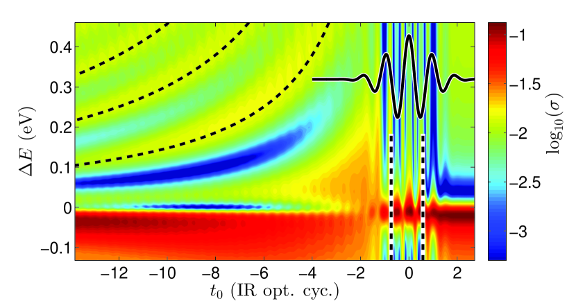
Figure 1: PES $\sigma(\Delta E)$ in the vicinity of the 2s2p resonance as a function of XUV excitation time $t_{0}$ ($l=1$ partial wave). IR peak intensity $2\times 10^{12}W/cm^{2}$. Solid line: IR field, curved fine-dashed lines: $2n\pi\hbar/|t_{0}|,n=1,2,3$, closely follow interference maxima. Negative $t_{0}$ correpsond to the XUV preceding IR. Dashed vertical lines indicate the lineout times of Fig. 2.

We first present the PES in the vicinity of the He(2s2p) line as a function of XUV excitation time $t_{0}$ with an IR pulse centered at $t=0$ (Fig. 1). The results were obtained by numerically solving the time-dependent Schrödinger equation of the He atom in full 3+3 spatial dimensions. Spectra were computed using the time-dependent surface flux method (tSURFF, Tao and Scrinzi (2012); Scrinzi (2012)). For a summary of the computational approach and discussion of its accuracy, see Majety et al. (2015). The XUV center wavelength of $\lambda=21\,nm$ was chosen to match the excitation to the $2s2p$ state, but the spectral width of $\sim 10\,eV$ at the pulse duration of $0.15\,fs$ evenly covers the entire $2s\mathrm{n}p$ series of doubly excited He states. The calculations were performed for IR wavelength of $800\,nm$ with a pulse duration of 2 optical cycles, peak intensity $2\times 10^{12}W/cm^{2}$, and parallel linear polarization of the XUV and IR pulses.

The two lineouts (Fig. 2) pertain to $t_{0}=-3/4$ and $+1/2$ (in units of IR optical cycle). At $t_{0}=-3/4$, where the XUV pulse coincides with a node of the IR electric field, one sees a strongly asymmetric Fano profile. In contrast, at $t=+1/2$, peak of the IR field, the profile is Lorentz-like. Neither the width nor the position of the resonance are affected by the weak IR. The pattern is repeated as $t_{0}$ is scanned through the IR pulse.

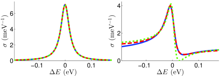
Figure 2: PES at two different delay times as indicated in Fig. 1. Left: $t_{0}=1/2$ IR opt.cyc., near a field peak, right: $t_{0}=-3/4$, near a field node. IR peak intensity $10^{12}W/cm^{2}$. Solid: numerical result, dashed: fit admitting complex $q$, dot-dashed: fit with $q$ restricted to real. All three lines nearly coincide at $t_{0}=1/2$.

Fig. 2 also contains fits to the lines by Eq. (1), where $\Gamma$ was taken from the IR-free case. Only the overall intensity $\sigma_{0}$ and the $q$-parameter and were adjusted, either restricting $q$ to real values and or admitting complex $q$, respectively. When the XUV coincides with a node of the IR (right panel of Fig. 2), only the fit with complex $q$ is satisfactory: there is no exact zero in the spectrum when IR and XUV pulse overlap, which trivially rules out an accurate fit by Eq. (1) with real $q$.

For the example of PES we show how complex $q$ arises in the framework of a generalized Fano theory. A standard Fano Hamiltonian has the form

$$H=|\varphi\rangle E_{\varphi}\langle\varphi|+\!\!\int|{\vec{k}}\rangle\frac{k^{2}}{2}\langle{\vec{k}}|+|{\vec{k}}\rangle V_{\vec{k}}\langle\varphi|+|\varphi\rangle V_{\vec{k}}^{*}\langle{\vec{k}}|\mathrm{d}^{3}k,$$ (3)

where the embedded bound state $|\varphi\rangle$ interacts with the continuum states $|{\vec{k}}\rangle$ through $V_{\vec{k}}=\langle{\vec{k}}|V|\varphi\rangle$. Solutions are known for the exact scattering eigenfunctions $|\xi_{\vec{k}}\rangle$, the resonance width $\Gamma$, and the shift of the resonance position from the non-interacting $E_{\varphi}$. The Fano transition amplitude $\langle\xi_{\vec{k}}|T|\phi_{0}\rangle$ for an arbitrary transition operator $T$ from some initial state $|\phi_{0}\rangle$ leads to the Fano cross section (1). We introduce the wave packet after transition

$$T|\phi_{0}\rangle=:|\psi_{0}\rangle=|\varphi\rangle X_{\varphi}+\int{\color[rgb]{0,0,0}\mathrm{d}}^{3}k\,|{\vec{k}}\rangle X_{\vec{k}},$$ (4)

with the transition amplitudes from the initial state $X_{\varphi}=\langle\varphi|T|\phi_{0}\rangle$ and $X_{\vec{k}}=\langle{\vec{k}}|T|\phi_{0}\rangle$. For notational simplicity we consider the case where $|\varphi\rangle$ decays into a well-defined angular momentum state, in case of the 2s2p doubly excited state this is the $l=1$ partial wave. The $q$-parameter for the standard Fano Hamiltonian (3), denoted as $q_{0}$, is

$$q_{0}=\frac{1}{\pi V_{k}^{*}k}\frac{\langle\varphi|\psi_{0}\rangle+\mathcal{P}\int k^{\prime 2}{\color[rgb]{0,0,0}\mathrm{d}}k^{\prime}\frac{2V^{*}_{k^{\prime}}}{k^{2}-k^{\prime 2}}\langle k^{\prime}|\psi_{0}\rangle}{\langle k|\psi_{0}\rangle},$$ (5)

where the $|k\rangle$ denotes the $l=1$ partial wave continuum states with $k=\sqrt{{\vec{k}}^{2}}$ and $V_{k}$ are the coupling matrix elements between embedded and continuum states. When the $\langle k^{\prime}|\psi_{0}\rangle$ and $\langle\varphi|\psi_{0}\rangle$ all share the same phase, $q$ is real.

In our model for the transition in the pulse overlap region, we assume that the initial state $|\phi_{0}\rangle$ is unaffected by the IR and that the effect on the embedded state $|\varphi\rangle$ is only a Stark shift $\Delta E_{\varphi}(t)$ relative to the field-free energy $E_{\varphi}$. The interaction of the IR with the continuum states is described in the standard “strong field approximation” Lewenstein et al. (1994): when the IR field prevails over the atomic potential, the continuum states at time $t$ can be approximated as plane waves with wave vector ${\vec{k}}-{\vec{A}}(t)$ and the phase of the time-evolution is modified accordingly. Finally, we assume that the IR pulse duration is short compared to the decay time of the embedded state. With that the net effect of the IR pulse is to replace $|\psi_{0}\rangle$ by a modified initial wave packet

$$|\psi_{1}\rangle=|\varphi\rangle X_{\varphi}+\int{\color[rgb]{0,0,0}\mathrm{d}}^{3}k\,{\color[rgb]{0,0,0}\mathrm{e}}^{-{\color[rgb]{0,0,0}\mathrm{i}}\Phi_{\vec{k}}}|{\vec{k}}\rangle X_{{\vec{k}}-{\vec{A}}(t_{0})}$$ (6)

(see Supplemental Material sup ). The phase offset $\Phi_{\vec{k}}$ between embedded and continuum states accumulated from excitation at $t_{0}$ until the end of the IR pulse at $t_{1}$, ${\vec{A}}(t_{1})=0$, is

$${\color[rgb]{0,0,0}\Phi_{{\vec{k}}}={\int_{t_{0}}^{t_{1}}\mathrm{d}\tau}\,\Big{(}[{\vec{k}}-{\vec{A}}(\tau)]^{2}/2-E_{\varphi}-\Delta E_{\varphi}(\tau)\Big{)}}.$$ (7)

Clearly, even if the initial amplitudes $X_{\varphi}$ and $X_{{\vec{k}}-{\vec{A}}(t_{0})}$ are all real, the interaction with the IR imprints a phase-modulation on $|\psi_{1}\rangle$ and the Fano parameter becomes complex. Moreover, in $X_{{\vec{k}}-{\vec{A}}(t_{0})}$ the partial waves are redistributed compared to the IR-free $X_{\vec{k}}$ by the addition of a streaking momentum ${\vec{A}}(t_{0})$. A short calculation (see sup ) leads to the IR modification of the Fano parameter

$$q_{1}=q_{0}+a\left(\mathrm{e}^{-\mathrm{i}\chi}/\mathcal{J}-1\right),$$ (8)

where $a=\langle\varphi|\psi_{0}\rangle/(\pi V^{*}_{k}k\langle k|\psi_{0}\rangle)$ denotes the ratio of embedded to continuum amplitudes without the IR, and

$${\color[rgb]{0,0,0}\chi=\int_{t_{0}}^{t_{1}}\mathrm{d}\tau\,\left[\Delta E_{\varphi}(\tau)-\vec{A}^{2}(\tau)/2\right]}$$ (9)

is a laser-induced phase shift between the two components. Although the phase-shift $\chi$ does give a numerically discernable contribution, the $t_{0}$-dependence of $q_{1}$ is dominated by

$$\mathcal{J}=j_{0}(|{\vec{\alpha}}|k)-2j_{2}(|{\vec{\alpha}}|k)-3\mathrm{i}\frac{j_{1}\left(|{\vec{\alpha}}|k\right)}{|{\vec{\alpha}}|k}\,{\vec{\alpha}}\cdot{\vec{A}}(t_{0}),$$ (10)

where the spatial offset of a free electron by the IR pulse

$${\vec{\alpha}}=\int_{t_{0}}^{t_{1}}{\color[rgb]{0,0,0}\mathrm{d}\tau}\,{\vec{A}}(\tau)$$ (11)

appears in the argument of the spherical Bessel functions $j_{l}$. The $\mathcal{J}$-term accounts for streaking by the term $\int_{t_{0}}^{t_{1}}{\vec{k}}\cdot{\vec{A}}(\tau)d\tau$ in $\Phi_{\vec{k}}$. By the dipole selection rule $|\psi_{0}\rangle$ has angular momentum $l=1$ and therefore only the $j_{0}$, $j_{1}$, and $j_{2}$ contribute to the $l=1$ partial wave emission.

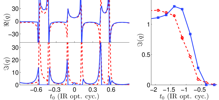
Figure 3: Dependence of $q_{1}$ on XUV-IR delay time $t_{0}$ according to Eq. (8) (dashed lines) and from fits to numerical results (solid lines). Upper panel: $\Re(q_{1})$, lower panel: $\Im(q_{1})$. Right: $\Im(q_{1})$ at times $t_{n}$ near the nodes of the field (${\vec{\alpha}}=0$, see text): Eq. (8) (bullets) and fit (squares).

In Fig. 3 we compare Eq. (8) with fits to the numerically computed 2s2p line. For the fits, the amplitude ratio was kept constant at the field-free value of $a=-3.3$ and Stark shifts were neglected, $\Delta E_{\varphi}\equiv 0$. Sign changes of the real part and peaks in the imaginary parts are all well reproduced. Quantitative deviations must be expected in the strong field approximation, for example, due to the use of plane waves $|\vec{k}\rangle$ instead of the exact scattering solutions. In addition, there is a non-negligible IR two-photon coupling, as will be discussed below.

There are excitation times $t_{0}=t_{n}$ where the spatial offset vanishes, ${\vec{\alpha}}=0$, and therefore $\mathcal{J}=1$. At these delays, the imaginary part of $q_{1}$ is exclusively due to the phase-shifts $\chi$. Up to small corrections arising from the short IR pulse duration, the $t_{n}$ coincide with zeros of the field. At the $t_{n}$ the profile is Fano-like (Fig. 2), except that the characteristic minimum remains slightly above zero. In our model, the minima for subsequent $t_{n}$’s grow monotonically as the delay $|t_{0}|$ increases (Fig. 3, right panel) reflecting the accumulation of the shift $\chi$, Eq. (9). For overlapping pulses, all resonances $2s\mathrm{n}p$, $n=2$ through 7 show the same delay-dependence, which corroborates that line-shape modulations are dominated by the dressing of the continuum.

When the XUV precedes the IR pulse without overlap (large negative $t_{0}$), the spatial offset goes to zero (${\vec{\alpha}}\approx 0$) and therefore $\mathcal{J}\approx 1$. Here, line-shapes are the combined effect of the phase-shift $\chi$ and IR two-photon coupling between embedded and continuum states. Two-photon coupling is not included in the standard Fano model Eq. (3). It manifests itself in side-band like interferences. Stimulated 2-IR-photon emission creates ripples in the otherwise smooth non-resonant PES around the energies $E_{-}=E_{\varphi}-2\omega$, where $\omega$ is the IR photon energy. The electron amplitude generated by two-photon absorption near $E_{+}=E_{\varphi}+2\omega$ is super-imposed with the higher-lying Fano resonances and therefore not clearly discernable. Absorption-emission transitions couple the embedded state to the continuum near $E=E_{\varphi}$. We model the spectral features near $E_{\beta},\,\beta=\varphi$ and $\beta=-$ by

$$\sigma(E) = |f(E)+\mathcal{E}_{0}^{2}e^{-it_{0}(E-E_{\beta})}b_{\beta}(E)|^{2},$$ (12)

where $t_{0}$ is the XUV-IR delay, $\mathcal{E}_{0}$ denotes the IR peak field strength, and $f(E)$ is the spectral amplitude in absence of the IR. The unknown two-IR-photon transition amplitudes are parameterized as $b_{\beta}(E)=c_{\beta}g(E-E_{\beta})$. For $g$ we use a Gaussian profile with a fixed width equal to the spectral width of the IR. The only adjustable parameters are the two-photon coupling strengths $c_{\beta}$, accounting for the different strengths of the transition into structured and unstructured continuum.

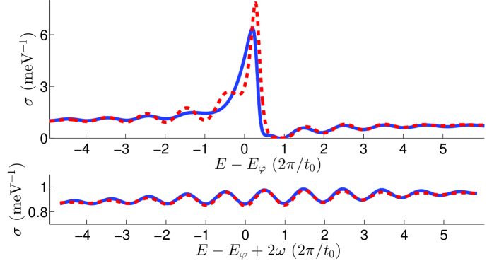
Figure 4: Two-photon interference resonance in the $l=1$ partial wave near $E_{\varphi}$ (upper panel) and near $E_{\varphi}-2\omega$ (lower). Cross-section Eq. (12) (dot-dashed) is compared to the full numerical result (solid) at $t_{0}=-12$ opt.cyc.

In Fig. 4 the cross-section Eq. (12) at $t_{0}=-12$ IR opt.cyc. is compared to the TDSE result. The fringe separation of $2\pi/t_{0}$ discernable in Figs.1 and 4 proves that the structures are caused by interference of photo-electrons emitted at relative delay $t_{0}$. Without any further adjustment of $c_{\beta}$ or $g$ the model equally well reproduces the spectra for varying intensities up to $I\lesssim 10^{12}W/cm^{2}$ and for all $t_{0}$. The quadratic dependence on IR field strength $\mathcal{E}_{0}$ shows that this is a true two-photon process without resonant coupling to neighboring states. At short time-delays $t_{0}$ the effect is negligible, as fringe separation diverges and fringes are hardly discernable.

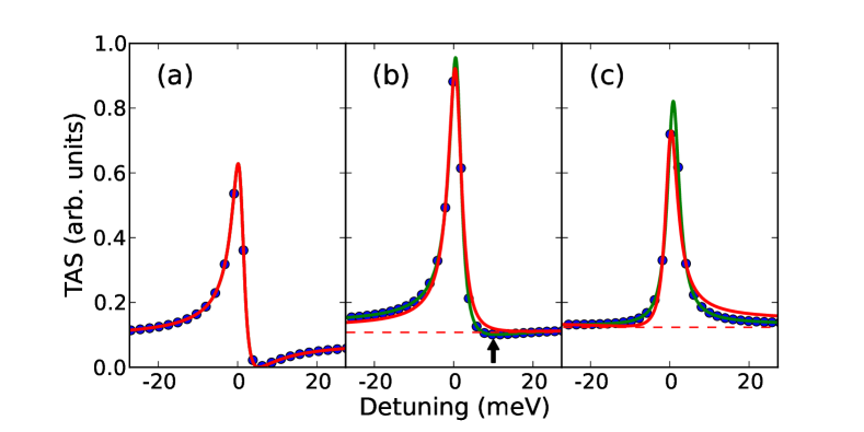
Figure 5: TAS at the $2s4p$ resonance. Results are shown for (a) XUV only, (b) a $7\,fs$ FWHM IR pulse with peak intensity $I=2\times 10^{12}W/cm^{2}$ reached at arrival of the XUV pulse, and (c) the peak IR intensity $5\,fs$ after the XUV. Dots: numerical results; green lines: fit of a Fano profile with complex $q$ (arrow marks the local minimum), solid red lines: Fano profile with real $q$ according Ott et al. (2013) and additional offset indicated by the dashed red line.

Turning now to the complementary channels for observing Fano line shapes by the IR field we calculate TAS near the $2s\mathrm{n}p$, $n\leq 6$ states using the pulse parameters of Ref. Ott et al. (2013). The spectra were determined from the full TDSE solutions following the method described in Ref. Gaarde et al. (2011).

The delay dependence of the TAS differs from that of the PES: under the influence of the IR field the characteristic minimum of the Fano line all but disappears and does not fully reappear for delays shorter than the resonance life time. Fig. 5 shows as an example the computed transient absorption line of the $n=4$ resonance at different IR delays. In all cases the numerical results conform with a generalized Fano line with a complex $q$ parameter. For comparison, we include the Fano shapes with the purely real $q$-parameter predicted in Ott et al. (2013), where a constant pedestal of absorption was admitted to account for the offset of the lines from zero. The point to be noted is that the present numerical calculation is background-free, i.e., such a pedestal cannot be explained by a background contribution from other channels. The weak local minimum seen in the numerically computed absorption line at delay 0 corresponds to complex $q=-1.2+i2.4$. This is at variance with real valued $q=-9$ resulting from the model proposed in Ott et al. (2013). Both, the offset from zero and the absorption minimum in the vicinity of the peak indicate that the influence of the control field is not fully captured by the model of Ott et al. (2013).

The complex $q$ in TAS and PES appears at parameters that are accessible by experimental setups as in Ref. Ott et al. (2013). For either observable the signature of complex $q$ is a local minimum above 0. For PES the shape should follow Eq. (8), for TAS the exact shape can be obtained numerically. The main experimental difficulty obviously is the proper background subtraction. In case of the PES, the presence of the IR introduces a smooth background of partial waves, Eq. (2), in addition to the $l=1$ partial wave that exhibits the Fano interference. However, at the times $t_{n}$ where $\vec{\alpha}=0$ the contributions from the other partial waves are negligible and $\Im(q)$ as given in the right panel in Fig. 3 is directly observable in the angle-integrated cross section. At other delays, the $l=1$ cross section must be reconstructed from an angle-resolved measurement (see, e.g., Garcia et al. (2004)).

In summary, anomalous Fano profiles with complex $q$-parameter appear whenever a non-trivial relative phase between embedded state and continuum is imprinted on the system during the Fano decay. Such a phase can reflect internal dynamics of the embedded state $|\varphi\rangle$, i.e. when it is not strictly an eigenstate of a stationary Hamiltonian, as for decaying states and de-coherence. It can equally be generated by an external control, as demonstrated here. Our theoretical description of the process should be generalizable to systems where we can model the impact of the control on bound and embedded states and when control time is short compared to the resonance life time. This is the case for laser pulses on atoms or molecules, but the approach is also valid, e.g., for time-dependent electric or magnetic fields acting on quantum dots.

We acknowledge support by the excellence cluster “Munich Center for Advanced Photonics (MAP)” and by the Austrian Science Foundation project ViCoM (F41) and NEXTLITE (F049).

References

- Fano (1961) U. Fano, Phys. Rev. 124, 1866 (1961).
- Miroshnichenko et al. (2010) A. E. Miroshnichenko, S. Flach, and Y. S. Kivshar, Rev. Mod. Phys. 82, 2257 (2010), URL http://link.aps.org/doi/10.1103/RevModPhys.82.2257.
- Kobayashi et al. (2003) K. Kobayashi, H. Aikawa, S. Katsumoto, and Y. Iye, Phys. Rev. B 68, 235304 (2003), URL http://link.aps.org/doi/10.1103/PhysRevB.68.235304.
- Lee (1999) H.-W. Lee, Phys. Rev. Lett. 82, 2358 (1999), URL http://link.aps.org/doi/10.1103/PhysRevLett.82.2358.
- Agarwal et al. (1984) G. S. Agarwal, S. L. Haan, and J. Cooper, Phys. Rev. A 29, 2552 (1984), URL http://link.aps.org/doi/10.1103/PhysRevA.29.2552.
- Wickenhauser et al. (2005) M. Wickenhauser, J. Burgdoerfer, F. Krausz, and M. Drescher, Phys. Rev. Lett. 94, 023002 (2005).
- Clerk et al. (2001) A. A. Clerk, X. Waintal, and P. W. Brouwer, Phys. Rev. Lett. 86, 4636 (2001), URL http://link.aps.org/doi/10.1103/PhysRevLett.86.4636.
- Bärnthaler et al. (2010) A. Bärnthaler, S. Rotter, F. Libisch, J. Burgdörfer, S. Gehler, U. Kuhl, and H.-J. Stöckmann, Phys. Rev. Lett. 105, 056801 (2010), URL http://link.aps.org/doi/10.1103/PhysRevLett.105.056801.
- Ott et al. (2013) C. Ott, A. Kaldun, P. Raith, K. Meyer, M. Laux, J. Evers, C. H. Keitel, C. H. Greene, and T. Pfeifer, Science 340, 716 (2013).
- Zhao and Lin (2005) Z. X. Zhao and C. D. Lin, Phys. Rev. A 71, 060702 (2005), URL http://link.aps.org/doi/10.1103/PhysRevA.71.060702.
- Chu and Lin (2013) W.-C. Chu and C. D. Lin, Phys. Rev. A 87, 013415 (2013).
- Zhao and Lein (2012) J. Zhao and M. Lein, New Journal of Physics 14, 065003 (2012).
- Chu et al. (2014) W.-C. Chu, T. Morishita, and C. D. Lin, Phys. Rev. A 89, 033427 (2014), URL http://link.aps.org/doi/10.1103/PhysRevA.89.033427.
- Tao and Scrinzi (2012) L. Tao and A. Scrinzi, New Journal of Physics 14, 013021 (2012).
- Scrinzi (2012) A. Scrinzi, New Journal of Physics 14, 085008 (2012), ISSN 1367-2630.
- Majety et al. (2015) V. P. Majety, A. Zielinski, and A. Scrinzi, New Journal of Physics 17, 063002 (2015), URL http://stacks.iop.org/1367-2630/17/i=6/a=063002.
- Lewenstein et al. (1994) M. Lewenstein, P. Balcou, M. Y. Ivanov, A. L’Huillier, and P. B. Corkum, Phys. Rev. A 49, 2117 (1994).
- (18) Supplemental material: derivation of eq. (8).
- Gaarde et al. (2011) M. B. Gaarde, C. Buth, J. L. Tate, and K. J. Schafer, Phys. Rev. A 83, 013419 (2011), URL http://link.aps.org/doi/10.1103/PhysRevA.83.013419.
- Garcia et al. (2004) G. A. Garcia, L. Nahon, and I. Powis, Rev. Sci. Instrum. 75, 4989 (2004).