Stochastic order relations among parallel systems
from Weibull distributions

Abstract

Let $X_{\lambda_{1}},X_{\lambda_{2}},\ldots,X_{\lambda_{n}}$ be independent Weibull random variables with $X_{\lambda_{i}}\sim W(\alpha,\lambda_{i})$ where $\lambda_{i}>0$, for $i=1,\ldots,n$. Let $X_{n:n}^{\lambda}$ denote the lifetime of the parallel system formed from $X_{\lambda_{1}},X_{\lambda_{2}},\ldots,X_{\lambda_{n}}$. We investigate the effect of the changes in the scale parameters $(\lambda_{1},\ldots,\lambda_{n})$ on the magnitude of $X_{n:n}^{\lambda}$ according to reverse hazard rate and likelihood ratio orderings.

Keywords: likelihood ratio order; reverse hazard rate order; majorization; order statistics; multiple-outlier model

Mathematics Subject Classification (2010) 62G30 ; 60E15 ; 60K10

1 Introduction

There is an extensive literature on stochastic orderings among order statistics and spacings when the observations follow the exponential distribution with different scale parameters, see for instance, Dykstra et al. (1997); Bon and Păltănea (1999); Khaledi and Kochar (2000); Wen et al. (2007); Zhao et al. (2009); Torrado and Lillo (2013) and the references therein. Also see a review paper by Kochar (2012) on this topic. A natural way to extend these works is to consider random variables with Weibull distributions since it includes exponential distributions.

Let $X_{\lambda_{1}},X_{\lambda_{2}},\ldots,X_{\lambda_{n}}$ be independent Weibull random variables with $X_{\lambda_{i}}\sim W(\alpha,\lambda_{i})$, $i=1,\ldots,n$, where $\lambda_{i}>0,i=1,\ldots,n$, i.e., with density function

$$f_{i}(t)=\alpha\lambda_{i}\left(\lambda_{i}t\right)^{\alpha-1}e^{-\left(\lambda_{i}t\right)^{\alpha}},\text{ }t>0.$$

Let $h_{i}$ and $r_{i}$ be the hazard rate and the reverse hazard rate functions of $X_{\lambda_{i}}$, respectively. We denote by $X_{n:n}^{\lambda}$ the lifetime of the parallel system formed from $X_{\lambda_{1}},X_{\lambda_{2}},\ldots,X_{\lambda_{n}}$. Then, its distribution function is given by

$$F_{n:n}^{\lambda}(t)=\prod\limits_{i=1}^{n}F_{i}(t),$$

its density function is

$$f_{n:n}^{\lambda}(t)=\prod\limits_{i=1}^{n}F_{i}(t)\sum_{i=1}^{n}r_{i}(t),$$

and its reverse hazard rate function is

$$r_{n:n}^{\lambda}(t)=\sum_{i=1}^{n}r_{i}(t)=\sum_{i=1}^{n}\frac{\alpha\lambda_{i}\left(\lambda_{i}t\right)^{\alpha-1}}{e^{\left(\lambda_{i}t\right)^{\alpha}}-1}.$$ (1.1)

For $0<\alpha\leq 1$, Khaledi and Kochar (2006) proved that order statistics from Weibull distributions with a common shape parameter and with scale parameters as $(\lambda_{1},\ldots,\lambda_{n})$ and $(\theta_{1},\ldots,\theta_{n})$ are ordered in the usual stochastic order if one vector of scale parameters majorizes the other one. For the proportional hazard rate model, they also investigated the hazard rate and the dispersive orders among parallel systems of a set of $n$ independent and non-identically distributed random variables with that corresponding to a set of $n$ independent and identically distributed random variables. Similar results for Weibull distributions are also obtained by Fang and Zhang (2012).

In this article, we focus on stochastic orders to compare the magnitudes of two parallel systems from Weibull distributions when one set of scale parameters majorizes the other. The new results obtained here extend some of those proved by Dykstra et al. (1997) and Joo and Mi (2010) from exponential to Weibull distributions. Also, we present some results for parallel systems from multiple-outlier Weibull models.

The rest of the paper is organized as follows. In Section 2, we give the required definitions. We present some useful lemmas in Section 3 which are used throughout the paper . In the last section we establish some new results on likelihood ratio ordering among parallel systems from Weibull distributions.

2 Basic definitions

In this section, we review some definitions and well-known notions of stochastic orders and majorization concepts. Throughout this article increasing means non-decreasing and decreasing means non-increasing.

Let $X$ and $Y$ be univariate random variables with cumulative distribution functions (c.d.f.’s) $F$ and $G$, survival functions $\bar{F}\left(=1-F\right)$ and $\bar{G}\left(=1-G\right)$, p.d.f.’s $f$ and $g$, hazard rate functions $h_{F}\left(=f/\,\bar{F}\right)$ and $h_{G}\left(=g/\,\bar{G}\right)$, and reverse hazard rate functions $r_{F}\left(=f/F\right)$ and $r_{G}\left(=g/G\right)$, respectively. The following definitions introduce stochastic orders, which are considered in this article, to compare the magnitudes of two random variables. For more details on stochastic comparisons, see Shaked and Shanthikumar (2007).

Definition 2.1

We say that $X$ is smaller than $Y$ in the:

• usual stochastic order, denoted by $X\leq_{st}Y$ or $F\leq_{st}G$, if $\bar{F}(t)\leq\bar{G}(t)$ for all $t$,

• hazard rate order, denoted by $X\leq_{hr}Y$ or $F\leq_{hr}G$, if $\bar{G}(t)/\,\bar{F}(t)$ is increasing in $t$ for all $t$ for which this ratio is well defined,

• reverse hazard rate order, denoted by $X\leq_{rh}Y$ or $F\leq_{rh}G$, if $G(t)/F(t)$ is increasing in $t$ for all $t$ for which the ratio is well defined,

• likelihood ratio order, denoted by $X\leq_{lr}Y$ or $F\leq_{lr}G$, if $g(t)/f(t)$ is increasing in $t$ for all $t$ for which the ratio is well defined.

In this paper, we shall be using the following Theorem 1.C.4 of Shaked and Shanthikumar (2007).

(a) If $X\leq_{hr}Y$ and if $\frac{h_{Y}(t)}{h_{X}(t)}$ increases in $t$, then $X\leq_{lr}Y$.

(b) If $X\leq_{rh}Y$ and if $\frac{r_{Y}(t)}{r_{X}(t)}$ increases in $t$, then $X\leq_{lr}Y$.

We shall also be using the concept of majorization in our discussion. Let $\{x_{(1)},x_{(2)},\ldots,x_{(n)}\}$ denote the increasing arrangement of the components of the vector ${\bm{x}}=\left(x_{1},x_{2},\ldots,x_{n}\right)$.

Definition 2.2

The vector ${\bm{x}}$ is said to be majorized by the vector ${\bm{y}}$, denoted by ${\bm{x}}\leq^{m}{\bm{y}}$, if

$$\sum_{i=1}^{j}x_{(i)}\geq\sum_{i=1}^{j}y_{(i)},\quad\text{for }j=1,\ldots,n-1\quad\text{ and }\quad\sum_{i=1}^{n}x_{(i)}=\sum_{i=1}^{n}y_{(i)}.$$

Functions that preserve the ordering of majorization are said to be Schur-convex as defined below.

Definition 2.3

A real valued function $\varphi$ defined on a set $\mathcal{A}\in\Re^{n}$ is said to be Schur-convex (Schur-concave) on $\mathcal{A}$ if

$${\bm{x}}\leq^{m}{\bm{y}}\,\text{on }\,\mathcal{A}\Rightarrow\varphi({\bm{x}})\leq(\geq)\varphi({\bm{y}}).$$

A concept of weak majorization is the following.

Definition 2.4

The vector ${\bm{x}}$ is said to be weakly majorized by the vector ${\bm{y}}$, denoted by ${\bm{x}}\leq^{w}{\bm{y}}$, if

$$\sum_{i=1}^{j}x_{(i)}\geq\sum_{i=1}^{j}y_{(i)},\quad\text{for }j=1,\ldots,n.$$

It is known that ${\bm{x}}\leq^{m}{\bm{y}}\Rightarrow{\bm{x}}\leq^{w}{\bm{y}}$. The converse is, however, not true. For extensive and comprehensive details on the theory of majorization orders and their applications, please refer to the book of Marshall et al. (2011).

3 Preliminaries results

In this section, we first preset several useful lemmas which will be used in the next section to prove our main results.

Lemma 3.1

For $t\geq 0$, the function

$$u(t)=\frac{t^{\alpha}}{e^{t^{\alpha}}-1}$$ (3.1)

is decreasing for any $\alpha>0$ and convex for $0<\alpha\leq 1$.

Proof. Note that, for $t\geq 0$, $u(t)=\psi_{1}(t^{\alpha})$ with

$$\psi_{1}(t)=\frac{t}{e^{t}-1}.$$

It is easy to check that $\psi_{1}(t)$ is a decreasing and convex function. Therefore,

$$\frac{d}{dt}u(t)=\alpha t^{\alpha-1}\frac{d}{dt}\psi_{1}(t)\leq 0$$

for any $\alpha>0$, and

$$\frac{d^{2}}{dt^{2}}u(t)=\alpha(\alpha-1)t^{\alpha-2}\frac{d}{dt}\psi_{1}(t)+\left(\alpha t^{\alpha-1}\right)^{2}\frac{d^{2}}{dt^{2}}\psi_{1}(t)\geq 0,$$

since $0<\alpha\leq 1$. Hence $u(t)$ is decreasing for any $\alpha>0$ and convex for $0<\alpha\leq 1$ in $[0,\infty).$   

Lemma 3.2

For $t\geq 0$, the function

$$v(t)=\frac{t^{\alpha}}{1-e^{-t^{\alpha}}}$$ (3.2)

is increasing for any $\alpha>0$.

Proof. Note that, for $t\geq 0$, $v(t)=\psi_{2}(t^{\alpha})$ with

$$\psi_{2}(t)=\frac{t}{1-e^{-t}}.$$

As shown by Khaledi and Kochar (2000) in Lemma 2.1, $\psi_{2}(t)$ is increasing in $t\geq 0$. Hence $v(t)$ is also increasing because

$$\frac{d}{dt}v(t)=\alpha t^{\alpha-1}\frac{d}{dt}\psi_{2}(t)\geq 0\text{,}$$

for any $\alpha>0$.   

Lemma 3.3

For $t\geq 0$, the function

$$\frac{te^{t}(1+t-e^{t})}{(e^{t}-1)^{3}}$$ (3.3)

is increasing.

Proof. The derivative of (3.3) is, for $t\geq 0$,

$$\frac{e^{t}}{(e^{t}-1)^{4}}(-1+e^{2t}(t-1)-t(3+t)+e^{t}(2-2t(t-1))).$$

Thus, it is sufficient to prove that

$$M_{1}(t)=-1+e^{2t}(t-1)-t(3+t)+e^{t}(2-2t(t-1))\geq 0.$$

Since $M_{1}(0)=0$, we have to prove that

$$M_{1}^{\prime}(t)=e^{2t}(2t-1)-3-20+2e^{t}(2-t(1+t))\geq 0.$$

Again, $M_{1}^{\prime}(0)=0$, so we have to prove that

$$M_{1}^{\prime\prime}(t)=2(-1+e^{t}(1-t(3-2e^{t}+t)))\geq 0.$$

Denote, for $t\geq 0$,

$$M_{2}(t)=-1+e^{t}(1-t(3-2e^{t}+t)).$$

Since the derivative of $M_{2}(t)$ is,

$$M_{2}^{\prime}(t)=e^{t}(-2-t(5+t)+e^{t}(2+4t))$$

and $e^{t}\geq 1+t$, it follows that $M_{2}^{\prime}(t)\geq 0$, because

$$-2-t(5+t)+e^{t}(2+4t)\geq-2-t(5+t)+(1+t)(2+4t)=t(1+3t)\geq 0.$$

That is, $M_{2}(t)$ is increasing in $t\geq 0$. Observing that $M_{2}(0)=0$, we have $M_{2}(t)\geq 0$ for $t\geq 0$. The required result follows immediately.   

Lemma 3.4

For $t\geq 0$, the function

$$w(t)=\frac{\alpha t^{2\alpha-1}e^{t^{\alpha}}(1+t^{\alpha}-e^{t^{\alpha}})}{(e^{t^{\alpha}}-1)^{3}}$$ (3.4)

is increasing for $0<\alpha\leq 1$.

Proof. Note that, for $t\geq 0$,

$$w(t)=\alpha t^{\alpha-1}\psi_{3}(t^{\alpha}),$$

with

$$\psi_{3}(t)=\frac{te^{t}(1+t-e^{t})}{(e^{t}-1)^{3}}.$$

From Lemma 3.3 we know that $\psi_{3}(t)$ is an increasing function, then

$$\frac{d}{dt}w(t)=\alpha(\alpha-1)t^{\alpha-2}\psi_{3}(t^{\alpha})+\left(\alpha t^{\alpha-1}\right)^{2}\frac{d}{dt}\psi_{3}(t)\geq 0,$$

since $0<\alpha\leq 1$ and $\psi_{3}(t)\leq 0$ because $e^{t}\geq 1+t$ for $t\geq 0$. Hence $w(t)$ is increasing in $[0,\infty)$ for $0<\alpha\leq 1.$   

4 Main results

In this section, we establish likelihood ratio ordering between parallel systems based on two sets of heterogeneous Weibull random variables with a common shape parameter and with scale parameters which are ordered according to a majorization order. First, we establish a comparison among parallel systems according to reverse hazard rate ordering when the common shape parameter $\alpha$ satisfies $0<\alpha\leq 1$.

Theorem 4.1

Let $X_{\lambda_{1}},X_{\lambda_{2}},\ldots,X_{\lambda_{n}}$ be independent random variables with $X_{\lambda_{i}}\sim W(\alpha,\lambda_{i})$, where $\lambda_{i}>0$, $i=1,\ldots,n$, and let $X_{\theta_{1}},X_{\theta_{2}},\ldots,X_{\theta_{n}}$ be another set of independent random variables with $X_{\theta_{i}}\sim W(\alpha,\theta_{i})$, where $\theta_{i}>0$, $i=1,\ldots,n$. Then for $0<\alpha\leq 1$,

$$\left(\lambda_{1},\ldots,\lambda_{n}\right)\preceq^{w}\left(\theta_{1},\ldots,\theta_{n}\right)\Rightarrow X_{n:n}^{\lambda}\leq_{rh}X_{n:n}^{\theta}.$$

Proof. Fix $t\geq 0$. Then the reverse hazard rate of $X_{n:n}$ is

$$r_{n:n}^{\lambda}(t)=\frac{\alpha}{t}\sum_{i=1}^{n}\frac{\left(\lambda_{i}t\right)^{\alpha}}{e^{\left(\lambda_{i}t\right)^{\alpha}}-1}=\frac{\alpha}{t}\sum_{i=1}^{n}u(\lambda_{i}t),$$

where $u(t)$ is defined as in (3.1). From Theorem A.8 of Marshall et al. (2011) (p.59) it suffices to show that, for each $t\geq 0$, $r_{n:n}^{\lambda}(t)$ is decreasing in each $\lambda_{i}$, $i=1,\ldots,n$, and is a Schur-convex function of $\left(\lambda_{1},\ldots,\lambda_{n}\right)$. It is well known that the hazard rate of the Weibull distribution is decreasing in $t\geq 0$ when $0<\alpha\leq 1$ (see Marshall and Olkin (2007), p. 324), and therefore, its reverse hazard rate function is also decreasing. Clearly, from (1.1), the reverse hazard rate function of $X_{n:n}$ is decreasing in each $\lambda_{i}$. Now, from Proposition C.1 of Marshall et al. (2011) (p. 64), in order to establish the Schur-convexity of $r_{n:n}^{\lambda}(t)$, it is enough to prove the convexity of $u(t)$. Note that, from Lemma 3.1, we know that $u(t)$ is a convex function for $0<\alpha\leq 1$. Hence $r_{n:n}^{\lambda}(t)$ is a Schur-convex function of $\left(\lambda_{1},\ldots,\lambda_{n}\right)$.   

Since ${\bm{x}}\leq^{m}{\bm{y}}\Rightarrow{\bm{x}}\leq^{w}{\bm{y}}$, the following corollary follows immediately from Theorem 4.1.

Corollary 4.2

Let $X_{\lambda_{1}},X_{\lambda_{2}},\ldots,X_{\lambda_{n}}$ be independent random variables with $X_{\lambda_{i}}\sim W(\alpha,\lambda_{i})$, where $\lambda_{i}>0$, $i=1,\ldots,n$, and let $X_{\theta_{1}},X_{\theta_{2}},\ldots,X_{\theta_{n}}$ be another set of independent random variables with $X_{\theta_{i}}\sim W(\alpha,\theta_{i})$, where $\theta_{i}>0$, $i=1,\ldots,n$. Then for $0<\alpha\leq 1$,

$$\left(\lambda_{1},\ldots,\lambda_{n}\right)\preceq^{m}\left(\theta_{1},\ldots,\theta_{n}\right)\Rightarrow X_{n:n}^{\lambda}\leq_{rh}X_{n:n}^{\theta}.$$

Note that Corollary 4.2 was proved by Khaledi et al. (2011) for generalized gamma distribution when $p=q<1$ which corresponds to Weibull distribution with shape parameter $\alpha<1$.

A natural question is whether the results of Theorem 4.1 and Corollary 4.2 can be strengthened from reverse hazard rate ordering to likelihood ratio ordering. First we consider the case when $n=2$.

Theorem 4.3

Let $X_{\lambda_{1}},X_{\lambda_{2}}$ be independent random variables with $X_{\lambda_{i}}\sim W(\alpha,\lambda_{i})$ where $\lambda_{i}>0$, $i=1,2$, and let $X_{\theta_{1}},X_{\theta_{2}}$ be independent random variables with $X_{\theta_{i}}\sim W(\alpha,\theta_{i})$ where $\theta_{i}>0$, $i=1,2$. Then

$$\left(\lambda_{1},\lambda_{2}\right)\preceq^{m}\left(\theta_{1},\theta_{2}\right)\Rightarrow\frac{r_{2:2}^{\theta}(t)}{r_{2:2}^{\lambda}(t)}\text{ is increasing in }t\text{, for }0<\alpha\leq 1.$$

Proof. From (1.1) we have

$$r_{2:2}^{\theta}(t)=\frac{\alpha}{t}\left(\frac{\left(\theta_{1}t\right)^{\alpha}}{e^{(\theta_{1}t)^{\alpha}}-1}+\frac{\left(\theta_{2}t\right)^{\alpha}}{e^{(\theta_{2}t)^{\alpha}}-1}\right),$$

then

$$\phi(t)=\frac{r_{2:2}^{\theta}(t)}{r_{2:2}^{\lambda}(t)}=\frac{u(\theta_{1}t)+u(\theta_{2}t)}{u(\lambda_{1}t)+u(\lambda_{2}t)},$$

where $u(t)$ is the function defined in (3.1). Note that the derivative of $u(t)$ with respect to $t$ is

$$u^{\prime}(t)=\frac{\alpha t^{\alpha-1}\left(e^{t^{\alpha}}-1-t^{\alpha}e^{t^{\alpha}}\right)}{\left(e^{t^{\alpha}}-1\right)^{2}}=\frac{\alpha}{t}u(t)s(t),$$

where

$$s(t) = \frac{-1+e^{t^{\alpha}}(1-t^{\alpha})}{e^{t^{\alpha}}-1}=1-\frac{t^{\alpha}e^{t^{\alpha}}}{e^{t^{\alpha}}-1}$$

$$= 1-\frac{t^{\alpha}}{1-e^{-t^{\alpha}}}=1-v(t),$$

with $v(t)$ defined as in (3.2). Therefore, from Lemma 3.2, we know that$\ s(t)$ is a decreasing function. We have to show that $\phi^{\prime}(t)\geq 0$ for all $t\geq 0$. The derivative of $\phi(t)$ is, for $t\geq 0$,

$$\phi^{\prime}(t) \overset{\text{sign}}{=} \left(u(\theta_{1}t)s(\theta_{1}t)+u(\theta_{2}t)s(\theta_{2}t)\right)\left(u(\lambda_{1}t)+u(\lambda_{2}t)\right)$$

$$-\left(u(\theta_{1}t)+u(\theta_{2}t)\right)\left(u(\lambda_{1}t)s(\lambda_{1}t)+u(\lambda_{2}t)s(\lambda_{2}t)\right).$$

Thus, we have to prove that the function

$$L\left(\theta_{1},\theta_{2}\right)=\frac{pu(\theta_{1}t)s(\theta_{1}t)+qu(\theta_{2}t)s(\theta_{2}t)}{pu(\theta_{1}t)+qu(\theta_{2}t)}$$

is Schur-convex in $\left(\theta_{1},\theta_{2}\right)$. On differentiating $L\left(\theta_{1},\theta_{2}\right)$ with respect to $\theta_{1}$, we get

$$\frac{dL\left(\theta_{1},\theta_{2}\right)}{d\theta_{1}} \overset{\text{sign}}{=} \left[u^{\prime}(\theta_{1}t)s(\theta_{1}t)+u(\theta_{1}t)s^{\prime}(\theta_{1}t)\right]\left[u(\theta_{1}t)+u(\theta_{2}t)\right]$$

$$-\left[u(\theta_{1}t)s(\theta_{1}t)+u(\theta_{2}t)s(\theta_{2}t)\right]u^{\prime}(\theta_{1}t)$$

$$= u(\theta_{2}t)u^{\prime}(\theta_{1}t)\left[s(\theta_{1}t)-s(\theta_{2}t)\right]+u(\theta_{1}t)s^{\prime}(\theta_{1}t)\left[u(\theta_{1}t)+u(\theta_{2}t)\right].$$

Note that $u(t)s^{\prime}(t)=w(t)$ which is defined in (3.3) and from Lemma 3.3, we know that $w(t)$ is an increasing function for $0<\alpha\leq 1$. Then, (4) can be rewritten as

$$\frac{dL\left(\theta_{1},\theta_{2}\right)}{d\theta_{1}}\overset{\text{sign}}{=}u(\theta_{2}t)u^{\prime}(\theta_{1}t)\left[s(\theta_{1}t)-s(\theta_{2}t)\right]+w(\theta_{1}t)\left[u(\theta_{1}t)+u(\theta_{2}t)\right].$$

By interchanging $\theta_{1}$ and $\theta_{2}$, we have

$$\frac{dL\left(\theta_{1},\theta_{2}\right)}{d\theta_{2}}\overset{\text{sign}}{=}u(\theta_{1}t)u^{\prime}(\theta_{2}t)\left[s(\theta_{2}t)-s(\theta_{1}t)\right]+w(\theta_{2}t)\left[u(\theta_{1}t)+u(\theta_{2}t)\right].$$

Thus,

$$\frac{dL\left(\theta_{1},\theta_{2}\right)}{d\theta_{1}}-\frac{dL\left(\theta_{1},\theta_{2}\right)}{d\theta_{2}} \overset{\text{sign}}{=} \left[s(\theta_{1}t)-s(\theta_{2}t)\right]\left[u(\theta_{2}t)u^{\prime}(\theta_{1}t)+u(\theta_{1}t)u^{\prime}(\theta_{2}t)\right]+$$

$$\left[u(\theta_{1}t)+u(\theta_{2}t)\right]\left[w(\theta_{1}t)-w(\theta_{2}t)\right]$$

$$\leq 0,$$

if $\theta_{1}\leq\theta_{2}$, since $s(t)$ is decreasing, $u^{\prime}(t)\leq 0$ because $u(t)$ is a decreasing function and $w(t)$ is an increasing function. Hence,

$$\left(\theta_{1}-\theta_{2}\right)\left(\frac{dL\left(\theta_{1},\theta_{2}\right)}{d\theta_{1}}-\frac{dL\left(\theta_{1},\theta_{2}\right)}{d\theta_{2}}\right)\geq 0.$$

 

In the next result, we extend Theorem 4.1 from reverse hazard rate ordering to likelihood ratio ordering for $n=2$.

Theorem 4.4

Let $X_{\lambda_{1}},X_{\lambda_{2}}$ be independent random variables with $X_{\lambda_{i}}\sim W(\alpha,\lambda_{i})$ where $\lambda_{i}>0$, $i=1,2$, and let $X_{\theta_{1}},X_{\theta_{2}}$ be independent random variables with $X_{\theta_{i}}\sim W(\alpha,\theta_{i})$ where $\theta_{i}>0$, $i=1,2$. Then for $0<\alpha\leq 1$,

$$\left(\lambda_{1},\lambda_{2}\right)\preceq^{m}\left(\theta_{1},\theta_{2}\right)\Rightarrow X_{2:2}^{\lambda}\leq_{lr}X_{2:2}^{\theta}.$$

Proof. The required result follows from Theorem 1.C.4 in Shaked and Shanthikumar (2007) and Theorems 4.1 and 4.3.   

Note that Theorem 4.4 generalizes and strengthens Theorem 3.1 of Dykstra et al. (1997) from exponential to Weibull distributions.

One may wonder whether one can extend Theorem 4.4 for $\alpha>1$. The following example gives a negative answer.

Example 4.5

Let $\left(X_{\lambda_{1}},X_{\lambda_{2}}\right)$ be a vector of heterogeneous Weibull random variables, $W(\alpha,\lambda_{i})$, with $\alpha=2$ and scale parameter vector $\left(1.5,2\right)$. Let $\left(X_{\theta_{1}},X_{\theta_{2}}\right)$ be a vector of heterogeneous Weibull random variables, $W(\alpha,\theta_{i})$, with $\alpha=2$ and scale parameter vector $\left(1,2.5\right)$. Obviously $\left(\lambda_{1},\lambda_{2}\right)\preceq^{m}\left(\theta_{1},\theta_{2}\right)$, however $X_{2:2}^{\lambda}\nleq_{lr}X_{2:2}^{\theta}$ since $f_{2:2}^{\theta}(t)/f_{2:2}^{\lambda}(t)$ is not increasing in $t$ as it can be seen from Figure 1.

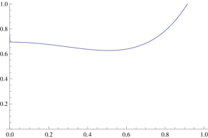
Figure 1: Plot of the $f_{n:n}^{\theta}(t)/f_{n:n}^{\lambda}(t)$ when $\alpha=2$, $\theta=\left(1,2.5\right)$ and $\lambda=\left(1.5,2\right)$ for random variables with Weibull distributions

For comparing the lifetimes of two parallel systems with independent Weibull components, $W(\alpha,\lambda_{i})$, we have proved in Theorem 4.4 that they are ordered according to likelihood ratio ordering under the condition of majorization order with respect to $(\lambda_{1},\lambda_{2})$ when $0<\alpha\leq 1$. For $n>2$, the problem is still open. However, in the multiple-outlier Weibull model, a similar result still holds. But first, we need to prove the following result.

Theorem 4.6

Let $X_{{1}},\ldots,X_{{n}}$ be independent random variables following the multiple-outlier Weibull model such that $X_{{i}}\sim W(\alpha,\lambda_{1})$ for $i=1,\ldots,p$ and $X_{{j}}\sim W(\alpha,\lambda_{2})$ for $j=p+1,\ldots,n$, with $\lambda_{1},\lambda_{2}>0$. Let $Y_{{1}},\ldots,Y_{{n}}$ be another set of independent random variables following the multiple-outlier Weibull model such that $Y_{{i}}\sim W(\alpha,\theta_{1})$ for $i=1,\ldots,p$ and $Y_{{j}}\sim W(\alpha,\theta_{2})$ for $j=p+1,\ldots,n$, with $\theta_{1},\theta_{2}>0$. Then for $0<\alpha\leq 1$,

$$(\underbrace{\lambda_{1},\ldots,\lambda_{1}}_{p},\underbrace{\lambda_{2},\ldots,\lambda_{2}}_{q})\preceq^{m}(\underbrace{\theta_{1},\ldots,\theta_{1}}_{p},\underbrace{\theta_{2},\ldots,\theta_{2}}_{q})\Rightarrow\frac{r_{n:n}^{\theta}(t)}{r_{n:n}^{\lambda}(t)}\text{ is increasing in }t,$$

where $p+q=n$.

Proof. From (1.1) we have

$$r_{n:n}^{\theta}(t)=\frac{\alpha}{t}\left(p\frac{\left(\theta_{1}t\right)^{\alpha}}{e^{(\theta_{1}t)^{\alpha}}-1}+q\frac{\left(\theta_{2}t\right)^{\alpha}}{e^{(\theta_{2}t)^{\alpha}}-1}\right),$$

where $p+q=n$, then

$$\phi(t)=\frac{r_{n:n}^{\theta}(t)}{r_{n:n}^{\lambda}(t)}=\frac{pu(\theta_{1}t)+qu(\theta_{2}t)}{pu(\lambda_{1}t)+qu(\lambda_{2}t)},$$

where $u(t)$ is the function defined in (3.1). We have to show that $\phi^{\prime}(t)\geq 0$ for all $t\geq 0$. The derivative of $\phi(t)$ is, for $t\geq 0$,

$$\phi^{\prime}(t) \overset{\text{sign}}{=} \left(pu(\theta_{1}t)s(\theta_{1}t)+qu(\theta_{2}t)s(\theta_{2}t)\right)\left(pu(\lambda_{1}t)+qu(\lambda_{2}t)\right)$$

$$-\left(pu(\theta_{1}t)+qu(\theta_{2}t)\right)\left(pu(\lambda_{1}t)s(\lambda_{1}t)+qu(\lambda_{2}t)s(\lambda_{2}t)\right),$$

where $s(t)=1-v(t)$ and $v(t)$ is defined in (3.2). Thus, we have to prove that the function

$$L\left(\theta_{1},\theta_{2}\right)=\frac{pu(\theta_{1}t)s(\theta_{1}t)+qu(\theta_{2}t)s(\theta_{2}t)}{pu(\theta_{1}t)+qu(\theta_{2}t)}$$

is Schur-convex in $\left(\theta_{1},\theta_{2}\right)$. On differentiating $L\left(\theta_{1},\theta_{2}\right)$ with respect to $\theta_{1}$, we get

$$\frac{dL\left(\theta_{1},\theta_{2}\right)}{d\theta_{1}} \overset{\text{sign}}{=} \left[u^{\prime}(\theta_{1}t)s(\theta_{1}t)+u(\theta_{1}t)s^{\prime}(\theta_{1}t)\right]\left[pu(\theta_{1}t)+qu(\theta_{2}t)\right]$$

$$-\left[pu(\theta_{1}t)s(\theta_{1}t)+qu(\theta_{2}t)s(\theta_{2}t)\right]u^{\prime}(\theta_{1}t)$$

$$= qu(\theta_{2}t)u^{\prime}(\theta_{1}t)\left[s(\theta_{1}t)-s(\theta_{2}t)\right]+u(\theta_{1}t)s^{\prime}(\theta_{1}t)\left[pu(\theta_{1}t)+qu(\theta_{2}t)\right].$$

Note that $u(t)s^{\prime}(t)=w(t)$ which is defined in (3.3) and from Lemma 3.3, we know that $w(t)$ is an increasing function for $0<\alpha\leq 1$. Then, (4) can be rewritten as

$$\frac{dL\left(\theta_{1},\theta_{2}\right)}{d\theta_{1}}\overset{\text{sign}}{=}qu(\theta_{2}t)u^{\prime}(\theta_{1}t)\left[s(\theta_{1}t)-s(\theta_{2}t)\right]+w(\theta_{1}t)\left[pu(\theta_{1}t)+qu(\theta_{2}t)\right].$$

By interchanging $\theta_{1}$ and $\theta_{2}$, we have

$$\frac{dL\left(\theta_{1},\theta_{2}\right)}{d\theta_{2}}\overset{\text{sign}}{=}pu(\theta_{1}t)u^{\prime}(\theta_{2}t)\left[s(\theta_{2}t)-s(\theta_{1}t)\right]+w(\theta_{2}t)\left[pu(\theta_{1}t)+qu(\theta_{2}t)\right].$$

Thus,

$$\frac{dL\left(\theta_{1},\theta_{2}\right)}{d\theta_{1}}-\frac{dL\left(\theta_{1},\theta_{2}\right)}{d\theta_{2}} \overset{\text{sign}}{=} \left[s(\theta_{1}t)-s(\theta_{2}t)\right]\left[qu(\theta_{2}t)u^{\prime}(\theta_{1}t)+pu(\theta_{1}t)u^{\prime}(\theta_{2}t)\right]+$$

$$\left[pu(\theta_{1}t)+qu(\theta_{2}t)\right]\left[w(\theta_{1}t)-w(\theta_{2}t)\right]$$

$$\leq 0,$$

if $\theta_{1}\leq\theta_{2}$, since $s(t)$ is decreasing, $u^{\prime}(t)\leq 0$ because $u(t)$ is a decreasing function and $w(t)$ is an increasing function. Hence,

$$\left(\theta_{1}-\theta_{2}\right)\left(\frac{dL\left(\theta_{1},\theta_{2}\right)}{d\theta_{1}}-\frac{dL\left(\theta_{1},\theta_{2}\right)}{d\theta_{2}}\right)\geq 0.$$

 

Using Theorems 4.1 and 4.6 and Theorem 1.C.4 in Shaked and Shanthikumar (2007), we have the following result.

Theorem 4.7

Let $X_{{1}},\ldots,X_{{n}}$ be independent random variables following the multiple-outlier Weibull model such that $X_{{i}}\sim W(\alpha,\lambda_{1})$ for $i=1,\ldots,p$ and $X_{{j}}\sim W(\alpha,\lambda_{2})$ for $j=p+1,\ldots,n$, with $\lambda_{1},\lambda_{2}>0$. Let $Y_{{1}},\ldots,Y_{{n}}$ be another set of independent random variables following the multiple-outlier Weibull model such that $Y_{{i}}\sim W(\alpha,\theta_{1})$ for $i=1,\ldots,p$ and $Y_{{j}}\sim W(\alpha,\theta_{2})$ for $j=p+1,\ldots,n$, with $\theta_{1},\theta_{2}>0$. Then for $0<\alpha\leq 1$,

$$(\underbrace{\lambda_{1},\ldots,\lambda_{1}}_{p},\underbrace{\lambda_{2},\ldots,\lambda_{2}}_{q})\preceq^{m}(\underbrace{\theta_{1},\ldots,\theta_{1}}_{p},\underbrace{\theta_{2},\ldots,\theta_{2}}_{q})\Rightarrow X_{n:n}^{\lambda}\leq_{lr}X_{n:n}^{\theta},$$

where $p+q=n$.

The above theorem says that the lifetime of a parallel system consisting of two types of Weibull components with a common shape parameter between 0 and 1 is stochastically larger according to likelihood ratio ordering when the scale parameters are more dispersed according to majorization.

In the following results, we investigate whether likelihood ratio ordering holds among parallel systems when the scale parameters of the Weibull distributions are ordered according to weak majorization order and the common shape parameter $\alpha$ is arbitrary.

Theorem 4.8

Let $X_{\lambda_{1}},X_{\lambda}$ be independent random variables with $X_{\lambda_{1}}\sim W(\alpha,\lambda_{1})$ and $X_{\lambda}\sim W(\alpha,\lambda)$ where $\lambda_{1},\lambda>0$. Let $Y_{\lambda_{1}^{\ast}},Y_{\lambda}$ be independent random variables with $Y_{\lambda_{1}^{\ast}}\sim W(\alpha,\lambda_{1}^{\ast})$ and $Y_{\lambda}\sim W(\alpha,\lambda)$, where $\lambda_{1}^{\ast},\lambda>0$. Suppose $\lambda_{1}^{\ast}=\min(\lambda,\lambda_{1},\lambda_{1}^{\ast})$, then for any $\alpha>0$,

$$\left(\lambda_{1},\lambda\right)\preceq^{w}\left(\lambda_{1}^{\ast},\lambda\right)\Rightarrow\frac{r_{2:2}^{\ast}(t)}{r_{2:2}(t)}\text{ is increasing in }t.$$

.

Proof. From (1.1), the reverse hazard rate function of $X_{2:2}$ is

$$r_{2:2}(t)=\frac{\alpha}{t}\left(\frac{\left(\lambda_{1}t\right)^{\alpha}}{e^{(\lambda_{1}t)^{\alpha}}-1}+\frac{\left(\lambda t\right)^{\alpha}}{e^{(\lambda t)^{\alpha}}-1}\right),$$

then

$$\phi(t)=\frac{r_{2:2}^{\ast}(t)}{r_{2:2}(t)}=\frac{\frac{(\lambda_{1}^{\ast}t)^{\alpha}}{e^{(\lambda_{1}^{\ast}t)^{\alpha}}-1}+\frac{(\lambda t)^{\alpha}}{e^{(\lambda t)^{\alpha}}-1}}{\frac{(\lambda_{1}t)^{\alpha}}{e^{(\lambda_{1}t)^{\alpha}}-1}+\frac{(\lambda t)^{\alpha}}{e^{(\lambda t)^{\alpha}}-1}}.$$

We have to show that $\phi^{\prime}(t)\geq 0$ for all $t\geq 0$. The derivative of $\phi(t)$ is, for $t\geq 0$,

$$\phi^{\prime}(t) \overset{\text{sign}}{=} \left(\frac{\alpha\lambda_{1}^{\ast}(\lambda_{1}^{\ast}t)^{\alpha-1}\left(e^{\left(\lambda_{1}^{\ast}t\right)^{\alpha}}-1-\left(\lambda_{1}^{\ast}t\right)^{\alpha}e^{\left(\lambda_{1}^{\ast}t\right)^{\alpha}}\right)}{\left(e^{\left(\lambda_{1}^{\ast}t\right)^{\alpha}}-1\right)^{2}}+\frac{\alpha\lambda(\lambda t)^{\alpha-1}\left(e^{\left(\lambda t\right)^{\alpha}}-1-\left(\lambda t\right)^{\alpha}e^{\left(\lambda t\right)^{\alpha}}\right)}{\left(e^{\left(\lambda t\right)^{\alpha}}-1\right)^{2}}\right)$$

$$\left(\frac{(\lambda_{1}t)^{\alpha}}{e^{(\lambda_{1}t)^{\alpha}}-1}+\frac{(\lambda t)^{\alpha}}{e^{(\lambda t)^{\alpha}}-1}\right)-\left(\frac{(\lambda_{1}^{\ast}t)^{\alpha}}{e^{(\lambda_{1}^{\ast}t)^{\alpha}}-1}+\frac{(\lambda t)^{\alpha}}{e^{(\lambda t)^{\alpha}}-1}\right)$$

$$\left(\frac{\alpha\lambda_{1}(\lambda_{1}t)^{\alpha-1}\left(e^{\left(\lambda_{1}t\right)^{\alpha}}-1-\left(\lambda_{1}t\right)^{\alpha}e^{\left(\lambda_{1}t\right)^{\alpha}}\right)}{\left(e^{\left(\lambda_{1}t\right)^{\alpha}}-1\right)^{2}}+\frac{\alpha\lambda(\lambda t)^{\alpha-1}\left(e^{\left(\lambda t\right)^{\alpha}}-1-\left(\lambda t\right)^{\alpha}e^{\left(\lambda t\right)^{\alpha}}\right)}{\left(e^{\left(\lambda t\right)^{\alpha}}-1\right)^{2}}\right).$$

After some computations, one get that

$$\phi^{\prime}(t) \overset{\text{sign}}{=} \frac{(\lambda_{1}^{\ast}t)^{\alpha}(\lambda_{1}t)^{\alpha}}{\left(e^{(\lambda_{1}^{\ast}t)^{\alpha}}-1\right)\left(e^{\left(\lambda_{1}t\right)^{\alpha}}-1\right)}\left(-\frac{\left(\lambda_{1}^{\ast}t\right)^{\alpha}}{\left(1-e^{-\left(\lambda_{1}^{\ast}t\right)^{\alpha}}\right)}+\frac{\left(\lambda_{1}t\right)^{\alpha}}{\left(1-e^{-\left(\lambda_{1}t\right)^{\alpha}}\right)}\right)$$

$$+\frac{(\lambda t)^{\alpha}(\lambda_{1}^{\ast}t)^{\alpha}}{\left(e^{(\lambda t)^{\alpha}}-1\right)\left(e^{\left(\lambda_{1}^{\ast}t\right)^{\alpha}}-1\right)}\left(-\frac{\left(\lambda_{1}^{\ast}t\right)^{\alpha}}{1-e^{-\left(\lambda_{1}^{\ast}t\right)^{\alpha}}}+\frac{\left(\lambda t\right)^{\alpha}}{1-e^{-\left(\lambda t\right)^{\alpha}}}\right)$$

$$+\frac{(\lambda_{1}t)^{\alpha}(\lambda t)^{\alpha}}{\left(e^{(\lambda_{1}t)^{\alpha}}-1\right)\left(e^{(\lambda t)^{\alpha}}-1\right)}\left(-\frac{\left(\lambda t\right)^{\alpha}}{\left(1-e^{-\left(\lambda t\right)^{\alpha}}\right)}+\frac{\left(\lambda_{1}t\right)^{\alpha}}{\left(1-e^{-\left(\lambda_{1}t\right)^{\alpha}}\right)}\right)$$

$$+\frac{(\lambda t)^{\alpha}(\lambda t)^{\alpha}}{\left(e^{(\lambda t)^{\alpha}}-1\right)\left(e^{\left(\lambda t\right)^{\alpha}}-1\right)}\left(-\frac{\left(\lambda t\right)^{\alpha}}{\left(1-e^{-\left(\lambda t\right)^{\alpha}}\right)}+\frac{\left(\lambda t\right)^{\alpha}}{\left(1-e^{-\left(\lambda t\right)^{\alpha}}\right)}\right).$$

By using the functions defined in (3.1) and (3.2), then the derivative of $\phi(t)$ can be rewritten by

$$\phi^{\prime}(t) \overset{\text{sign}}{=} u(\lambda_{1}^{\ast}t)u(\lambda_{1}t)\left(-v(\lambda_{1}^{\ast}t)+v(\lambda_{1}t)\right)+u(\lambda_{1}^{\ast}t)u(\lambda t)\left(-v(\lambda_{1}^{\ast}t)+v(\lambda t)\right)$$

$$+u(\lambda t)u(\lambda_{1}t)\left(-v(\lambda t)+v(\lambda_{1}t)\right).$$

Note that $u\left(t\right),v(t)\geq 0$ for all $t\geq 0$. From Lemmas 3.1 and 3.2, we know that $u\left(t\right)$ is decreasing and $v\left(t\right)$ is increasing in $t$. If $\lambda_{1}^{\ast}=\min(\lambda,\lambda_{1},\lambda_{1}^{\ast})$ and $\left(\lambda_{1},\lambda\right)\preceq^{w}\left(\lambda_{1}^{\ast},\lambda\right)$, then $\lambda_{1}^{\ast}\leq\lambda\leq\lambda_{1}$ or $\lambda_{1}^{\ast}\leq\lambda_{1}\leq\lambda$. When $\lambda_{1}^{\ast}\leq\lambda\leq\lambda_{1}$, we have $\phi^{\prime}(t)\geq 0$ since $v\left(\lambda_{1}^{\ast}t\right)\leq v\left(\lambda t\right)\leq v\left(\lambda_{1}t\right)$. When $\lambda_{1}^{\ast}\leq\lambda_{1}\leq\lambda$, we get

$$\phi^{\prime}(t) \geq u(\lambda t)u(\lambda_{1}t)\left(-v(\lambda_{1}^{\ast}t)+v(\lambda_{1}t)\right)+u(\lambda_{1}t)u(\lambda t)\left(-v(\lambda_{1}^{\ast}t)+v(\lambda t)\right)$$

$$+u(\lambda t)u(\lambda_{1}t)\left(-v(\lambda t)+v(\lambda_{1}t)\right)$$

$$= 2u(\lambda t)u(\lambda_{1}t)\left(-v(\lambda_{1}^{\ast}t)+v(\lambda_{1}t)\right)\geq 0\text{.}$$

Therefore $r_{2:2}^{\ast}(t)/r_{2:2}(t)$ is increasing in $t$ for any $\alpha>0$.   

Theorem 4.9

Let $X_{\lambda_{1}},X_{\lambda}$ be independent random variables with $X_{\lambda_{1}}\sim W(\alpha,\lambda_{1})$ and $X_{\lambda}\sim W(\alpha,\lambda)$ where $\lambda_{1},\lambda>0$. Let $Y_{\lambda_{1}^{\ast}},Y_{\lambda}$ be independent random variables with $Y_{\lambda_{1}^{\ast}}\sim W(\alpha,\lambda_{1}^{\ast})$ and $Y_{\lambda}\sim W(\alpha,\lambda)$, where $\lambda_{1}^{\ast},\lambda>0$. Suppose $\lambda_{1}^{\ast}=\min(\lambda,\lambda_{1},\lambda_{1}^{\ast})$, then for any $\alpha>0$,

$$\left(\lambda_{1},\lambda\right)\preceq^{w}\left(\lambda_{1}^{\ast},\lambda\right)\Rightarrow X_{2:2}\leq_{lr}Y_{2:2}.$$

Proof. From Theorem 4.8, we know that $r_{2:2}^{\ast}(t)/r_{2:2}(t)$ is increasing in $t$ under the given assumptions. Since $\left(\lambda_{1},\lambda\right)\preceq^{w}\left(\lambda_{1}^{\ast},\lambda\right)$, it follows from Theorem 4.1 that $X_{2:2}\leq_{rh}Y_{2:2}$. Thus the required result follows from Theorem 1.C.4 in Shaked and Shanthikumar (2007).   

Note that when $\left(\lambda_{1},\lambda\right)\preceq^{w}\left(\lambda_{1}^{\ast},\lambda\right)$ we have the following three possibilities:

$$\lambda_{1}^{\ast}\leq\lambda\leq\lambda_{1},\text{ }\lambda_{1}^{\ast}\leq\lambda_{1}\leq\lambda\text{ or }\lambda\leq\lambda_{1}^{\ast}\leq\lambda_{1}\text{.}$$

The two first are included in assumption of Theorem 4.9 and so a natural question is whether this theorem holds for $\lambda\leq\lambda_{1}^{\ast}\leq\lambda_{1}$. The following example gives a negative answer.

Example 4.10

Let $\left(X_{\lambda_{1}},X_{\lambda}\right)$ be a vector of heterogeneous Weibull random variables with $\alpha=0.3$ and scale parameters $\lambda=0.2$ and $\lambda_{1}=3.5$. Let $\left(Y_{\lambda_{1}^{\ast}},Y_{\lambda}\right)$ be a vector of heterogeneous Weibull random variables with $\alpha=0.3$ and scale parameters $\lambda=0.2$ and $\lambda_{1}^{\ast}=2$. Obviously $\left(\lambda_{1},\lambda\right)\preceq^{w}\left(\lambda_{1}^{\ast},\lambda\right)$ and $\lambda\leq\lambda_{1}^{\ast}\leq\lambda_{1}$. However $X_{2:2}\nleq_{lr}Y_{2:2}$ since $f_{2:2}^{\ast}(t)/f_{2:2}(t)$ is not increasing in $t$ as it can be seen from Figure 2. Analogously, from Figure 3, it can be seen that $X_{2:2}\nleq_{lr}Y_{2:2}$ when $\alpha=1.3$.

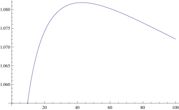
Figure 2: Plot of the $f_{2:2}^{*}(t)/f_{2:2}(t)$ when $\alpha=0.3$, $\lambda^{*}=\left(0.2,2\right)$ and $\lambda=\left(0.2,3.5\right)$ for random variables with Weibull distributions

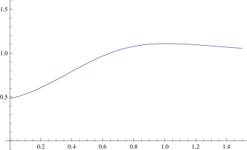
Figure 3: Plot of the $f_{2:2}^{*}(t)/f_{2:2}(t)$ when $\alpha=1.3$, $\lambda^{*}=\left(0.2,2\right)$ and $\lambda=\left(0.2,3.5\right)$ for random variables with Weibull distributions

From Theorems 4.9 and 4.4, the following result can be proved using arguments similar to those used in Theorem 3.6 of Zhao (2011).

Theorem 4.11

Let $X_{\lambda_{1}},X_{\lambda_{2}}$ be independent random variables with $X_{\lambda_{i}}\sim W(\alpha,\lambda_{i})$ where $\lambda_{i}>0$, $i=1,2$, and let $X_{\theta_{1}},X_{\theta_{2}}$ be another set of independent random variables with $X_{\theta_{i}}\sim W(\alpha,\theta_{i})$ where $\theta_{i}>0$, $i=1,2$. Suppose $\theta_{1}\leq\lambda_{1}\leq\lambda_{2}\leq\theta_{2}$. Then $\left(\lambda_{1},\lambda_{2}\right)\preceq^{w}\left(\theta_{1},\theta_{2}\right)$ implies that $X_{2:2}^{\lambda}\leq_{lr}X_{2:2}^{\theta}$, for $0<\alpha\leq 1$.

Note that Theorem 2.4 in Joo and Mi (2010) for two heterogeneous exponential random variables can be seen as a particular case of Theorem 4.11, since likelihood ratio order implies hazard rate order and exponential distributions are a particular case of Weibull distributions.

Next we extend the study of likelihood ratio ordering among parallel systems from the two-variable case to multiple-outlier Weibull models.

Theorem 4.12

Let $X_{1},\ldots,X_{n}$ be independent random variables following the multiple-outlier Weibull model such that $X_{i}\sim W(\alpha,\lambda_{1})$ for $i=1,\ldots,p$ and $X_{j}\sim W(\alpha,\lambda)$ for $j=p+1,\ldots,n$, with $\lambda_{1},\lambda>0$. Let $Y_{1},\ldots,Y_{n}$ be another set of independent random variables following the multiple-outlier Weibull model with $Y_{i}\sim W(\alpha,\lambda_{1}^{\ast})$ for $i=1,\ldots,p$ and $Y_{j}\sim W(\alpha,\lambda)$ for $j=p+1,\ldots,n$, with $\lambda_{1}^{\ast},\lambda>0$. Suppose $\lambda_{1}^{\ast}=\min(\lambda,\lambda_{1},\lambda_{1}^{\ast})$, then for any $\alpha>0$,

$$(\underbrace{\lambda_{1},\ldots,\lambda_{1}}_{p},\underbrace{\lambda,\ldots,\lambda}_{q})\preceq^{w}(\underbrace{\lambda_{1}^{\ast},\ldots,\lambda_{1}^{\ast}}_{p},\underbrace{\lambda,\ldots,\lambda}_{q})\Rightarrow\frac{r_{n:n}^{\ast}(t)}{r_{n:n}(t)}\text{ is increasing in }t,$$

where $p+q=n$.

Proof. From (1.1) we have the reverse hazard rate function of $X_{n:n}$

$$r_{n:n}(t)=\frac{\alpha}{t}\left(p\frac{\left(\lambda_{1}t\right)^{\alpha}}{e^{(\lambda_{1}t)^{\alpha}}-1}+q\frac{\left(\lambda t\right)^{\alpha}}{e^{(\lambda t)^{\alpha}}-1}\right),$$

where $p+q=n$. Let

$$\phi(t)=\frac{r_{n:n}^{\ast}(t)}{r_{n:n}(t)}=\frac{p\frac{(\lambda_{1}^{\ast}t)^{\alpha}}{e^{(\lambda_{1}^{\ast}t)^{\alpha}}-1}+q\frac{(\lambda t)^{\alpha}}{e^{(\lambda t)^{\alpha}}-1}}{p\frac{(\lambda_{1}t)^{\alpha}}{e^{(\lambda_{1}t)^{\alpha}}-1}+q\frac{(\lambda t)^{\alpha}}{e^{(\lambda t)^{\alpha}}-1}}.$$

As in the proof of Theorem 4.8, for $t\geq 0$, the derivative of $\phi(t)$ can be rewritten by

$$\phi^{\prime}(t) \overset{\text{sign}}{=} p^{2}u(\lambda_{1}^{\ast}t)u(\lambda_{1}t)\left(-v(\lambda_{1}^{\ast}t)+v(\lambda_{1}t)\right)+pqu(\lambda_{1}^{\ast}t)u(\lambda t)\left(-v(\lambda_{1}^{\ast}t)+v(\lambda t)\right)$$

$$+pqu(\lambda t)u(\lambda_{1}t)\left(-v(\lambda t)+v(\lambda_{1}t)\right).$$

Note that $u\left(t\right),v(t)\geq 0$ for all $t\geq 0$. From Lemmas 3.1 and 3.2, we know that $u\left(t\right)$ is decreasing and $v\left(t\right)$ is increasing in $t$. If $\lambda_{1}^{\ast}=\min(\lambda,\lambda_{1},\lambda_{1}^{\ast})$ and $\left(\lambda_{1},\lambda\right)\preceq^{w}\left(\lambda_{1}^{\ast},\lambda\right)$, then $\lambda_{1}^{\ast}\leq\lambda\leq\lambda_{1}$ or $\lambda_{1}^{\ast}\leq\lambda_{1}\leq\lambda$. When $\lambda_{1}^{\ast}\leq\lambda\leq\lambda_{1}$, we have $\phi^{\prime}(t)\geq 0$ since $v\left(\lambda_{1}^{\ast}t\right)\leq v\left(\lambda t\right)\leq v\left(\lambda_{1}t\right)$. When $\lambda_{1}^{\ast}\leq\lambda_{1}\leq\lambda$, we get

$$\phi^{\prime}(t) \geq p^{2}u(\lambda t)u(\lambda_{1}t)\left(-v(\lambda_{1}^{\ast}t)+v(\lambda_{1}t)\right)+pqu(\lambda_{1}t)u(\lambda t)\left(-v(\lambda_{1}^{\ast}t)+v(\lambda t)\right)$$

$$+pqu(\lambda t)u(\lambda_{1}t)\left(-v(\lambda t)+v(\lambda_{1}t)\right)$$

$$= npu(\lambda t)u(\lambda_{1}t)\left(-v(\lambda_{1}^{\ast}t)+v(\lambda_{1}t)\right)\geq 0\text{.}$$

Therefore $r_{n:n}^{\ast}(t)/r_{n:n}(t)$ is increasing in $t$ for any $\alpha>0$.   

Theorem 4.13

Let $X_{1},\ldots,X_{n}$ be independent random variables such that $X_{i}\sim W(\alpha,\lambda_{1})$ for $i=1,\ldots,p$ and $X_{j}\sim W(\alpha,\lambda)$ for $j=p+1,\ldots,n$, with $\lambda_{1},\lambda>0$. Let $Y_{1},\ldots,Y_{n}$ be independent nonnegative random variables with $Y_{i}\sim W(\alpha,\lambda_{1}^{\ast})$ for $i=1,\ldots,p$ and $Y_{j}\sim W(\alpha,\lambda)$ for $j=p+1,\ldots,n$, with $\lambda_{1}^{\ast},\lambda>0$. Suppose $\lambda_{1}^{\ast}=\min(\lambda,\lambda_{1},\lambda_{1}^{\ast})$, then

$$(\underbrace{\lambda_{1},\ldots,\lambda_{1}}_{p},\underbrace{\lambda,\ldots,\lambda}_{q})\preceq^{w}(\underbrace{\lambda_{1}^{\ast},\ldots,\lambda_{1}^{\ast}}_{p},\underbrace{\lambda,\ldots,\lambda}_{q})\Rightarrow X_{n:n}\leq_{lr}Y_{n:n},$$

for $p+q=n$ and any $\alpha>0$.

Proof. From Theorem 4.12, we know that under the given conditions,$r_{n:n}^{\ast}(t)/r_{n:n}(t)$ is increasing in $t$. Since $\left(\lambda_{1},\ldots,\lambda_{1},\lambda,\ldots,\lambda\right)\preceq^{w}\left(\lambda_{1}^{\ast},\ldots,\lambda_{1}^{\ast},\lambda,\ldots,\lambda\right)$, then $X_{n:n}\leq_{rh}Y_{n:n}$ from Theorem 4.1. Thus the required result follows from Theorem 1.C.4 in Shaked and Shanthikumar (2007).   

This result is similar to Theorem 4.7 without any restriction on the common shape parameter with but with an additional constraint on the scale parameters.

References

Bon and Păltănea (1999)Bon,
J.L. and Păltănea, E. (1999). Ordering
properties of convolutions of exponential random variables. Lifetime Data Analysis5, 185–192.
Dykstra et al. (1997)Dykstra,
S.C., Kochar, S.C. and Rojo, J. (1997). Stochastic
comparisons of parallel systems of heterogeneous exponential components. Journal of Statistical Planning and Inference65,
203–2011.
Fang and Zhang (2012)Fang, L. and Zhang, X. (2012). New results on stochastic
comparison of order statistics from heterogeneous Weibull populations. Journal of the Korean Statistical Society41,
13–16.
Joo and Mi (2010)Joo, S. and Mi, J. (2010). Some properties of hazard rate functions of
systems with two components. Journal of Statistical Planning
and Inference140, 444–453.
Khaledi and Kochar (2007)Khaledi,
B-E. and Kochar, S.C. (2007). Stochastic orderings
of order statistics of independent random variables with different scale
parameters. Communications in Statistics - Theory and Methods36, 1441–1449.
Khaledi and Kochar (2000)Khaledi,
B-E. and Kochar, S.C. (2000). Some new results on
stochastic comparisons of parallel systems. J. Appl. Probab37, 1123–1128.
Khaledi and Kochar (2006)Khaledi,
B-E. and Kochar, S.C. (2006). Weibull distribution:
some stochastic comparisons results. Journal of Statistical
Planning and Inference136, 3121–3129.
Khaledi et al. (2011)Khaledi,
B-E., Farsinezhad, S. and Kochar, S.C. (2011). Stochastic comarisons of order statistics in the scale model. Journal of Statistical Planning and Inference141, 276–286.
Kochar (2012)Kochar, S.C. (2012). Stochastic Comparisons of Order Statistics and Spacings: A Review. ISRN Probability and Statistics vol. 2012, Article ID
839473, 47 pages, 2012. doi:10.5402/2012/839473.
Marshall et al. (2011)Marshall, A. W., Olkin, I. and Arnold, B. C. (2011). Inequalities: Theory of majorization and its applications. New York: Springer.
Marshall and Olkin (2007)Marshall, A. W. and Olkin, I. (2007). Life
distributions. Springer, New York.
Shaked and Shanthikumar (2007)Shaked, M. and Shanthikumar, J. G. (2007). Stochastic Orders. Springer, New York.
Torrado and Lillo (2013)Torrado,
N. and Lillo, R.E. (2013). On stochastic properties
of spacings with applications in multiple-outlier models. In : Li,
H. and Li, X.(Ed.), Stochastic Orders in Reliability and Risk. Springer
Lecture Notes in Statistics, 103–123.
Zhao et al. (2009)Zhao, P., Li, X. and Balakrishnan, N. (2009). Likelihood ratio order
of the second order statistic from independent heterogeneous exponential
random variables. Journal of Multivariate Analysis100, 952–962.
Zhao (2011)Zhao, P. (2011). On parallel systems with heterogeneous gamma components. Probability in the Engineering and Informational Sciences25, 369–391.
Wen et al. (2007)Wen, S., Lu, Q. and Hu, T. (2007). Likelihood ratio orderings of
spacings of heterogeneous exponential random variables. Journal of Multivariate Analysis98, 743–756.