Localization length index in a Chalker-Coddington model: a numerical study

Abstract

We calculated numerically the localization length index $\nu$ for the Chalker-Coddington model of the plateau-plateau transitions in the quantum Hall effect. By taking into account finite size effects we have obtained $\nu=2.593\pm 0.0297$. The calculations were carried out by two different programs that produced close results, each one within the error bars of the other. We also checked the possibility of logarithmic corrections to finite size effects and found, that they come with much larger error bars for $\nu$.

The computation of critical indices of the plateau-plateau transitions in the quantum Hall effect (QHE) (see for a review Huckestein (1995)) is still an open problem in modern condensed matter physics. According to the pioneering works on localization Anderson (1958) the dimension two is a marginal dimension, above which delocalization can appear. Exactly at d=2 Levine, Libby and Pruisken Levine et al. (1984a, b, c) noticed, that the presence of a topological term in the nonlinear sigma model (NLSM) formulation of the problem may result in the appearance of delocalized states in strong magnetic fields. The next achievement was reached by Chalker and Coddington Chalker and Coddington (1988).

The authors formulated and studied numerically a network model ($CC$ model) in a random potential yielding localization-delocalization transitions. The numerical value $2.5\pm 0.5$ of the Lyapunov exponent (LE) in the CC model was in good agreement with the experimentally measured localization length index $\nu=2.4$ in the quantum Hall effect Wei et al. (1994). Recently the more precise value $\nu=2.38\pm 0.06$ was reported in Li et al. (2005, 2009).

Various aspects of the CC-model were investigated in a chain of interesting papers: In Lee (1994) the model was linked to replicated spin-chains, while in Zirnbauer (1994, 1997) its connection to supersymmetric spin-chains was revealed. Some links with conformal field theories of Wess-Zumino-Witten-Novikov (WZWN) type were presented in Tsvelik (2007) and LeClair (2001).

In Refs. Obuse et al. (2012); Evers et al. (2008) the authors investigated the multifractal behaviour of the CC model. Both papers reported quartic deviations from the exact quadratic dependence of the multifractal indices on the parameter $q$, which was predicted in Refs. Tsvelik (2007); LeClair (2001). This fact points out that the validity of the simple, supersymmetric WZWN approach to plateau-plateau transitions in the quantum Hall effect is questionable and here we are still far from the application of conformal field theory.

In spite of a lot of understanding that has been gained for the plateau-plateau transitions in the QHE, the final model which would allow for the calculation of the localization length index either analytically or numerically has not been formulated yet. Moreover, recently more precise numerical calculations of the localization length index of the CC-model Slevin and Ohtsuki (2009); Amado et al. (2011); Obuse et al. (2012); Dahlhaus et al. (2011) show values close to $2.61\pm 0.014$, which is well far from the experimental value $2.38\pm 0.06$ Li et al. (2009). This indicates that the CC-model as such is not applicable to the description of plateau transitions.

Figure 1: Schematic illustration of the CC network. $M_{1}$ and $M_{2}$ denote the column transfer matrices as defined in (1) and (2). Multiplication with a column transfer matrix describes the transition of a particle through the corresponding column of the lattice.

Up to now all numerical analyses of finite size scaling in the CC-model Slevin and Ohtsuki (2009); Amado et al. (2011); Obuse et al. (2012); Dahlhaus et al. (2011) show that the second, irrelevant operator in the model has a scaling dimension very close to the major one. Moreover, in  Amado et al. (2011) it was claimed that the next to leading order finite size resp. width $M$ corrections have $1/\log[M]$-form, which indicates for the CC-model the possible presence of two operators with almost equal conformal dimensions.

The goal of the current paper is threefold: First we want to recalculate the localization length index in order to test the results obtained in Slevin and Ohtsuki (2009); Amado et al. (2011); Obuse et al. (2012); Dahlhaus et al. (2011). Second we want to check whether the $1/\log[M]$-form for the corrections is adequate or not. Third we want to explore the possibility of two irrelevant fields in the scaling analysis.

To achieve these goals, we developed two independent codes to numerically investigate the finite size scaling of the CC-model. We calculated both the localization length index and the next to leading index.

For the calculation of critical indices we used the transfer-matrix method developed in MacKinnon and Kramer (1981, 1983). We had to calculate the smallest Lyapunov exponent (LE) of the CC-model, for which it was necessary to calculate a product $T_{L}=\prod_{j=1}^{L}M_{1}U_{1j}M_{2}U_{2j}$ of layers of transfer matrices $M_{1}U_{1j}M_{2}U_{2j}$ corresponding to two columns $M_{1}$, $M_{2}$ of vertical sequences of 2x2 scattering nodes, cp. Fig. 1:

$$M_{1}=\leavevmode\hbox to85.92pt{\vbox to69.79pt{\text{[drawing]}}} {B^{1}} {0} {0} {0} {B^{1}} {0} {0} {0} {B^{1}} \left.\vbox{\hrule height=33.64389pt,depth=33.64389pt,width=0.0pt}\right) \left(\vbox{\hrule height=33.64389pt,depth=33.64389pt,width=0.0pt}\right. {B^{1}} {0} {0} {0} {B^{1}} {0} {0} {0} {B^{1}} \left.\vbox{\hrule height=33.64389pt,depth=33.64389pt,width=0.0pt}\right) \left(\vbox{\hrule height=33.64389pt,depth=33.64389pt,width=0.0pt}\right.$$ (1)

and

$$M_{2}=\leavevmode\hbox to98.48pt{\vbox to82.26pt{\text{[drawing]}}} {B^{2}_{22}} {0} {0} {B^{2}_{21}} {0} {B^{2}} {0} {0} {B^{2}} {0} {B^{2}_{12}} {0} {0} {B^{2}_{11}} \left.\vbox{\hrule height=39.878pt,depth=39.878pt,width=0.0pt}\right) \left(\vbox{\hrule height=39.878pt,depth=39.878pt,width=0.0pt}\right. {B^{2}_{22}} {0} {0} {B^{2}_{21}} {0} {B^{2}} {0} {0} {B^{2}} {0} {B^{2}_{12}} {0} {0} {B^{2}_{11}} \left.\vbox{\hrule height=39.878pt,depth=39.878pt,width=0.0pt}\right) \left(\vbox{\hrule height=39.878pt,depth=39.878pt,width=0.0pt}\right.$$ (2)

with

$$B^{1}=\begin{pmatrix}1/t&r/t\\ r/t&1/t\end{pmatrix}\qquad\text{and}\qquad B^{2}=\begin{pmatrix}1/r&t/r\\ t/r&1/r\end{pmatrix}$$ (3)

where periodic boundary conditions were imposed on $M_{2}$. The $U$-matrices have a simple diagonal form: $\left[U_{1,2}\right]_{nm}=\exp{(i\alpha_{n})}\,\delta_{nm}$. Here $t$ and $r$ are the transmission and reflection amplitudes at each node of the regular lattice shown in Fig. 1 which are suitably parameterized by

$$t=\frac{1}{\sqrt{1+e^{2x}}}\qquad\text{and}\qquad r=\frac{1}{\sqrt{1+e^{-2x}}}.$$ (4)

The model parameter $x$ corresponds to the Fermi energy measured from the Landau band center scaled by the Landau band width (so the critical point is $x=0$) while the phases $\alpha_{n}$ are stochastic variables in the range $[0,2\pi)$, reflecting the randomness of the smooth electrostatic potential landscape.

We calculated the product of a chain of transfer matrices which contain random parameters. According to the Oceledec theorem Oseledec (1968) the $\frac{1}{L}$ power of the product has a set of eigenvalues, which are independent of the history of the randomness. The logarithms of the moduli of these eigenvalues are called Lyapunov exponents.

$$\gamma=\lim_{L\to\infty}\frac{\log[T_{L}T_{L}^{\dagger}]}{2L}\ ,$$ (5)

The smallest positive one of these exponents yields the critical behaviour of the correlation length of the model, i.e. $\gamma\sim x^{-\nu}$ where $\nu$ is the localization length index.

It is clear, that numerically the infinite limit cannot be calculated. For chains with finite length $L$, the central limit theorem Tutubalin (1965) tells us that the Lyapunov exponents have a Gaussian distribution with variance $\sigma_{\gamma}\sim\sqrt{\frac{M}{L}}$.

This means, that by considering a chain of length $L$ we calculate the LE with error $\sim\sqrt{\frac{M}{L}}$. Moreover, if we consider an ensemble of $N$ chains, the variance becomes $\sim\sqrt{\frac{M}{LN}}$. Therefore our strategy will be to consider large ensembles of chains.

We used ensembles of products with length $L$ ranging from $1\,000\,000$ to $5\,000\,000$. The details about our data base can be found in table 1.

$M$	$L$	number of products	program
20	1 000 000	900	Fortran
20	5 000 000	100	C++
40	1 000 000	1000	Fortran
40	5 000 000	350	C++
60	1 000 000	1000	Fortran
60	5 000 000	280	C++
80	1 000 000	1000	Fortran
80	5 000 000	380	C++
100	1 000 000	1020	Fortran
100	5 000 000	150	C++
120	1 000 000	850	Fortran
120	5 000 000	300	C++
140	1 000 000	1260	Fortran
140	5 000 000	310	C++
160	1 000 000	285	Fortran
160	5 000 000	220	C++
180	1 000 000	240	Fortran

Table 1: This table shows the statistics of the data. For each $M$ we have calculated the Lyapunov exponent with the 13 $x$-values that divide the interval $[0,0.08]$ into 12 equal parts.

Calculating these matrix products the naive way is not possible as many entries of the product very soon exceed the size of all available data types. One can overcome this problem by use of the method presented in MacKinnon and Kramer (1981, 1983), namely, the product can be performed with repeated QR decompositions. The rightmost $T$ is QR decomposed. The unitary Q is then multiplied with the next $T$ and the product is decomposed again. Repeating this procedure many times we are in principle left with some Q multiplied with a product of upper right triangular matrices. It appears, that the product of the diagonal entries of the upper triangular matrices are approaching the eigenvalues of the total transfer matrix $T_{L}$. Of these numbers we are only interested in those which are close to 1.

For details see for instance von Bremen et al. (1997). In our numerical simulations we found that it is also possible to apply the much faster LU decomposition instead of the QR decomposition.

I The fitting procedure

From the scaling behaviour of the Lyapunov exponent near the critical point we expect for finite size systems

$$\gamma M=\Gamma(M^{1/\nu}u_{0},f(M)\,u_{1}),$$ (6)

where $f(M)$ is decreasing with $M$. Here $M$ is the number of nodes in each column of the lattice. $u_{0}=u_{0}(x)$ is a relevant field and $u_{1}=u_{1}(x)$ the leading irrelevant field. It is common to choose $f(M)=M^{y}$, $y<0$. Further it is known, that the relevant field vanishes at the critical point. The left hand side was obtained from (5) dependent on the parametrization parameter $x$ and the lattice height $M$. The right hand side was expanded in a series in $x$ and $M$ and the coefficients were obtained by a fit. Some coefficients in this expansion need not to be taken into account as can be seen following the arguments of Slevin and Ohtsuki (2009):

If $x$ is replaced by $-x$ we see from (4) that $t$ turns into $r$ and vice versa. Due to the periodic boundary conditions the lattice is unchanged. Therefore the left hand side of (6) is invariant under a sign flip of $x$. Hence the right hand side must be even in $x$. That makes $u_{0}(x)$ and $u_{1}(x)$ even or odd. For the Chalker Coddington network the critical point is at $x=0$. This makes us choose $u_{o}(x)$ odd and $u_{1}(x)$ even. The fit now should use as few coefficients as possible while reproducing the data as good as possible.

One reasonable attempt is to do an expansion of the right hand side of (6) in $x$. This yields

$$\begin{split}\Gamma=&\;\Gamma_{00}+\sum_{k=1}^{\infty}\Gamma_{0k}\,M^{ky}\\ &+x^{2}\left[b_{2}\sum_{k=1}^{\infty}\Gamma_{01}\,M^{ky}+M^{2/\nu}\sum_{k=0}^{\infty}\Gamma_{2k}M^{ky}\right]\\ &+x^{4}\left[(b_{4}+b_{2}^{2})\sum_{k=1}^{\infty}\Gamma_{0k}M^{ky}+b_{2}M^{2/\nu}\sum_{k=1}^{\infty}\Gamma_{2k}M^{ky}\right.\\ &\qquad\ +\left.M^{4/\nu}\sum_{k=0}^{\infty}\Gamma_{4k}M^{ky}+a_{3}M^{2/\nu}\sum_{k=0}\Gamma_{2k}M^{ky}\right]\\ &+O(x^{6})\end{split}$$ (7)

A subset of this is the fitting formula used in Obuse et al. (2012). We tried both formulas and the one in (7) worked out better for our data.
The fitting formula above was derived by first expanding $\Gamma$ in the fields

$$\begin{split}\Gamma(u_{0}(x)&M^{1/nu},u_{1}(x)M^{y})=\Gamma_{00}+\Gamma_{01}u_{1}M^{y}\\ &+\Gamma_{20}u_{0}^{2}M^{2/\nu}+\Gamma_{02}u_{1}^{2}M^{2y}\\ &+\Gamma_{21}u_{0}^{2}u_{1}M^{2/\nu}M^{y}+\Gamma_{03}u_{1}^{3}M^{2y}\\ &+\Gamma_{40}u_{0}^{4}M^{4/\nu}+\Gamma_{22}u_{0}^{2}u_{1}^{2}M^{2y}+\Gamma_{04}u_{1}^{4}M^{4y}\\ &+\dots\end{split}$$ (8)

and then the fields in $x$ like it has been done by most other authors in the past

$$u_{o}(x)=x+\sum_{k=1}^{\infty}a_{2k+1}x^{2k+1}\quad\text{and}\quad u_{1}(x)=1+\sum_{k=1}^{\infty}b_{2k}x^{2k}$$ (9)

In (8) all coefficients in the expansion of $\Gamma$ that would contradict the scaling function being even in $x$ have been dropped. Because of ambiguity in the overall scaling of the fields, the leading coefficient in (9) can be chosen to be 1.
Of course the described expansion is unique, however when taking into account a finite number of expansion coefficients $\Gamma_{lk}$ and $a_{n}$, $b_{m}$, different fitting procedures can be devised. With formula (7) we obtained the best fits for our data.

We also considered the case of two irrelevant fields. This, in analogy to (6), gives

$${\gamma M=\Gamma(M^{1/\nu}u_{0},M^{y_{1}}\,u_{1},M^{y_{2}}\,u_{2}),\quad y_{1},y_{2}<0}$$ (10)

With the same reasoning as in the case of one irrelevant field we find that $\Gamma$ is even in $x$. Along the lines of the above case we obtain that $u_{0}$ is odd and $u_{1}$ and $u_{2}$ are even in $x$. Of course $\Gamma$ is even in $x$, too. This helps to identify expansion coefficients that are zero like in the case of one irrelevant field.

II Results

In Fig.2 we present the leading Lyapunov exponent for various numbers of $2\times 2$ blocks in the transfer matrix versus $x$ (defined by formulas (4)), which measures the deviation of the hopping parameters $r$ and $t$ from their critical value $1/\sqrt{2}$. The corresponding fitting parameters are presented in the table below.

In Fig.3 we present an example of the distribution of Lyapunov exponents with fixed $M$, product length $L$ and $x$. This distribution defines one point and its error for the fit. Here, we see a Gaussian distribution in full accordance with the central limit theorem Tutubalin (1965).

The fits have been performed with a trust region algorithm. In a first step the region for each parameter is chosen. Initial values within these regions are taken at random. The results are the initial values for the next fit without regional restrictions. These results are taken again as initial values. This is done recursively 200 times.

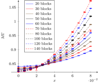
Figure 2: Plot of the smallest eigenvalue of the transfer matrix for different block sizes and in dependence on the distance $x$ from the critical point. The $x$-values divide the interval $[0,0.08]$ into 12 equal parts.

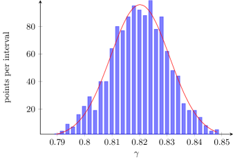
Figure 3: Distribution of Lyapunov exponents in the ensemble of calculations with 1282 elements for chain length $L=1\,000\,000$, $M=140$ and $x=0$

Our best fitting results have been obtained by taking the first two lines of (8) and expanding $u_{0}$ up to the third and $u_{1}$ up to the fourth order in $x$.

For the fitting formula :

$$\begin{split}M\Gamma(x,M)=\;&\Gamma_{00}+\Gamma_{01}*(1+b_{2}*x^{2})*(M^{y})\\ &+\Gamma_{20}*(x*M^{1/\nu})^{2}\\ &+\Gamma_{02}*((1+b_{2}*x^{2})*(M^{y}))^{2}\end{split}$$ (11)

we found the following coefficients and goodness of fit parameters :

Coefficients (confidence bounds 95%) :

$$\Gamma_{00}=\; \quad 0.737 (0.494 ,0.981)$$

$$\Gamma_{01}=\; \quad 0.185 (0.140 ,0.230)$$

$$\Gamma_{02}=\; \quad-0.0452 (-0.300 ,0.209)$$

$$\Gamma_{20}=\; \quad 0.863 (0.821 ,0.905)$$

$$b_{2}=\; -0.784 (-5.533 ,3.964)$$

$$\nu=\; \quad 2.59 (2.560 ,2.619)$$

$$y=\; -0.134 (-0.607 ,0.339)$$

Goodness of fit parameters :

sum of squares due to error : $$2.03664\cdot 10^{-7}$$

R-square : $$0.999925$$

degrees of freedom adjusted R-square : $$0.999924$$

root mean squared error : $$1.85167\cdot 10^{-5}$$

sum of residuals : $$0.00297$$

degrees of freedom : $$594$$

It turned out that the fit result depends slightly on the randomly chosen initial values. That means the parameters turn out different if we fit the same data several times. To take this into account we averaged over 200 fits as described above. Of course the averaged set of coefficients is not a good parameter set for the fit as all coefficients are highly correlated. So we just took the average for the critical index $\nu$. The distribution of $\nu$-values showed to have a Gaussian distribution. The average for $\nu$ gave :

$$\nu=2.593\pm 0.0297$$ (12)

Here the error is given by the standard deviation of the sample for the $\nu$-values. This result is in perfect agreement with the other recent work like Amado et al. (2011); Obuse et al. (2012); Slevin and Ohtsuki (2009). For $y$ we obtained analogously

$$y=-0.145\pm 0.0677$$ (13)

We have also found, that the fit with $1/\log(M)$ corrections does not give acceptably small confidence bounds for the main fitting value, the localization length index $\nu$. All attempts with different numbers of fitting coefficients did not lead to narrower confidence bounds.

Also potentially interesting is the ansatz with two irrelevant fields. It reproduces $\nu=2.6$ quite well, too. Averaging over an ensemble of fits similar to the case of one irrelevant field yields

$$\nu = 2.608\pm 0.0257$$ (14)

$$y_{1} = -0.728\pm 0.077$$ (15)

$$y_{2} = -0.733\pm 0.093$$ (16)

Again the error is given by the standard deviation of the ensemble of fits. $y_{1}$ and $y_{2}$ are quite similar in magnitude. We can neither explain why this is the case nor do we have a theoretical reason for the presence of two irrelevant fields. Identifying $y_{1}$ and $y_{2}$ is not equivalent with the case of a fit with one irrelevant field.

III conclusion and outlook

Our main result is in perfect agreement with the values of the localization length presented in the recent works Slevin and Ohtsuki (2009); Amado et al. (2011); Obuse et al. (2012); Dahlhaus et al. (2011).

We have also tested the goodness of the fit with $1/\log(M)$ corrections and found, that a power behaviour of the second, sub-leading term in the Lyapunov exponent is preferable, though it is very small, $y\sim-0.145$, indicating its proximity to $f(M)=1/\log(M)$ (see (6)) in the case of one irrelevant field.

We also successfully fitted two irrelevant fields. For this fit the confidence bounds are much wider but the result for $\nu$ is less affected by different choices for the range of values for $M$. As a fit with fewer coefficients is preferable we think that the ansatz with one irrelevant field is better. But we cannot rule out the possibility that indeed two irrelevant fields are important. It is clear that new and more extensive computations are needed to collect enough statistics for distinguishing the indices of the irrelevant operators with necessary precision.

The result confirms the necessity of an essential modification of the CC-model for the description of the plateau-plateau transition in the QHE.

Acknowledgments