Radial Stresses and Energy Transport in Accretion Disks

Abstract

Early in the study of viscous accretion disks it was realized that energy transfers from distant sources must be important, not least because the flow at the disk midplane in the bulk of the disk is likely outwards, out of the gravitational potential well. If the source of the viscosity is powered by accretion, such as in the case of the magneto-rotational instability, such distant energy sources must lie in the innermost regions of the disk, where accretion occurs even at the midplane. We argue here that modulations in this energy supply can alter the accretion rate on dynamical, rather than far longer viscous, time scales. This means that both the steady state value of and fluctuations in the inner disk’s accretion rate, depending on the details of the inner boundary condition and occurring on the inner disk’s rapid evolution time, can affect the outer disk. This is particularly interesting because observations have shown that disk accretion is not steady (e.g. EX Lupi type objects). We also note that the power supplied to shearing boxes is set by the boxes themselves rather than the physical energy fluxes in a global disk. That is, their saturated magnetic field is not subject to the full set of energy constraints present in an actual disk. Our analysis suggests that large scale radial transport of energy has a critical impact on the evolution and variability of accretion disks.

1. Introduction

Accretion disks surround many objects in the universe, from young stars, to compact binary companions, to supermassive black holes. Their observed accretion flows require outwards transport of angular momentum. The magnetic coupling of regions at different radii in accretion disks ranks high among the usual suspects for angular momentum transport mechanisms. This transport can occur either radially through the disk, such as with the magnetorotational instability (MRI, Balbus & Hawley, 1998), or vertically through a disk wind (Königl & Pudritz, 2000). Understanding vertical angular momentum transport through disk winds depends on understanding the disk’s vertical boundaries. Similarly, understanding radial angular momentum transport requires understanding the radial boundary conditions. In this paper, we argue that this is true not only near to but also far from those boundaries. While that may seem a trivial statement, in practice it means that even distant boundary conditions must be taken into account by numerical simulations intended to study the magnitude and direction of any accretion flows.

The common assumption of local control implicitly places any transition between accretion and decretion far from any region explicitly considered. Simulating regions far from any physically distinct radius further allows the use of the shearing box approximation, which goes so far as to erase the distinction between inwards and outwards directions. Balbus & Papaloizou (1999, hereafter BP99) found that the mean flow dynamics of MRI-driven MHD turbulence were a local phenomenon, justifying the use of alpha-disk models and shearing boxes.

It has long been known that steady state, vertically integrated, viscous, regions of accretion disks require an outwards energy flux in the standard theory (Lynden-Bell & Pringle, 1974). That theory defines $r_{b}$ as the position of the boundary layer where the differential rotation goes to zero (Frank et al., 2002). Protostars rotate below the Keplerian frequency, so $r_{b}$ must exist for disks that extend to the surface of their protostar, although it may not exist in strongly magnetized disks (Frank et al., 2002). It was shown early in the study of viscous disks that dissipation at radii $r>9r_{b}/4$ thermalizes significantly more energy than is released by the accretion flow there (Lynden-Bell & Pringle, 1974; Balbus & Hawley, 1998; Frank et al., 2002), with the balance made up by an energy flux built up within $9r_{b}/4$, and depleted over the entire outer disk.

Viscous disk theory predicts that disks decrete, rather than accrete, in regions where the stresses that drive accretion and angular momentum transport fall off faster with radius than $r^{-2}$ (Lynden-Bell & Pringle, 1974, BP99). In standard, self-similar disk models, this decretion condition is easily satisfied in disk midplanes where the pressure decreases rapidly with radius. It takes vertical integration through viscous disks to reliably find net accretion. This has led to the concept of meridional circulation, in which a decreting midplane is more than balanced by accreting surface layers (Urpin, 1984; Siemiginowska, 1988; Kley & Lin, 1992; Rozyczka et al., 1994; Regev & Gitelman, 2002; Takeuchi & Lin, 2002; Keller & Gail, 2004; Tscharnuter & Gail, 2007; Ciesla, 2007, 2009; Hughes & Armitage, 2010). Such behavior has been demonstrated in numerical models with a fixed anomalous viscosity defined by a constant Shakura-Sunyaev $\alpha$ parameter (Shakura & Sunyaev, 1973; Fromang et al., 2011).

These layered accretion structures arise in uniformly viscous disks because the disk thickness increases with radius in such disks. While the gas density and pressure in the midplane decrease with radius, they instead increase with cylindrical radius far enough above the midplane that the disk surface is encountered at finite radius. This occurs at increasing radius with height because the tilted disk surface reaches higher altitudes at larger radii. This transition in behavior is lost in slab geometries with radially constant scale height such as the shearing sheet approximation. In classical viscous disk theory the stress remains proportional to the gas pressure, so there exists a dividing height between decretion and accretion that occurs close to the surface, where the radial pressure gradient goes from falling off faster to falling off slower than $r^{-2}$ (e.g. Rozyczka et al., 1994).

Decreting regions of disks must be net importers of energy, since decretion boosts material out of a potential well. These regions still dissipate energy locally through non-ideal effects such as viscosity or resistivity, just as accretion regions do (Lynden-Bell & Pringle, 1974), but that just adds to the energy deficit that must be balanced by importing energy from inner regions. However, the source of that energy must be determined by the nature of the stresses driving accretion and decretion. If those stresses are powered by the accretion process itself and occur in the horizontal $r$-$\phi$ plane, as expected for magnetorational instability (Balbus & Hawley, 1991, 1998), We argue that this means that the midplane outflow of meridional circulation is powered not by the accreting upper layers, but rather by the inner edge of the midplane itself. Similar radial energy flows occur at every altitude, with the accreting inner edge of the disk at each altitude forming the accreting upper layer described by the meridional circulation picture.

BP99 argued that the mean flow dynamics of MRI-driven, MHD turbulence can be treated as a local phenomenon because the dynamical equations describing the flow are themselves local: the time derivatives at a specific spatial point of quantities such as the mean velocity or the mean magnetic field depend only on their values and spatial derivatives at that point. However, even distant regions of a disk will communicate on long enough time scales. This means that locality is more accurately treated as a time scale condition: on time scales shorter than some critical value, the disk can be treated as local, but it cannot be treated as local for longer time scales.

We show that the strength of the radial energy flows required to maintain the disk structure determine that critical time scale. The magnetic fields that provide the Maxwell stresses in MRI active disks have only a very small energy density, comparable to the accretion or decretion power integrated only over a few orbits. Order unity variations in the energy fluxes due to variability in the inner disk can therefore, everywhere within a few local orbits, cause order unity variations in the stresses, and hence the local accretion or decretion rates. This motivates us to extend the time dependent analysis in BP99 by including the time derivative of the stresses.

In Section 2 we revisit the basic equations for viscous disks. In Section 3 we discuss the energy fluxes present and estimate the dynamical time-scale associated with the stresses. In Section 4 we delve more deeply into the energy flux considerations in the context of the shearing sheet approximation, and discuss the difference between the case where stresses are powered by accretion energy (which includes most cases of turbulent viscosity) vs. the cases where the stresses are not powered by accretion energy (including many cases of microphysical viscosity). In Section 5 we discuss links to numerical simulations, both existing results and suggestions for future design and diagnostics. In Section 6 we place our results in context as an extension of the analysis of BP99, and we conclude in Section 7.

2. Angular Momentum Transport

2.1. Azimuthal Lorentz Forces

The action of the magnetic field on the gas to transfer angular momentum occurs through azimuthal Lorentz forces $\mbox{\boldmath$F$}{}_{L,\phi}=\mbox{\boldmath$J$}{}\times\mbox{\boldmath$B$}{}|_{\phi}$. In cylindrical coordinates, the magnetic field is

$$\mbox{\boldmath$B$}{}=B_{r}{\bm{\hat{e}}_{r}}+B_{\phi}{\bm{\hat{e}}_{\phi}}+B_{z}{\bm{\hat{e}}_{z}},$$ (1)

and the current density

$$\mu_{0}\mbox{\boldmath$J$}{}= \mbox{\boldmath$\nabla$}{}\times\mbox{\boldmath$B$}{},$$ (2)

$$= \left[\frac{1}{r}\partial_{\phi}B_{z}-\partial_{z}B_{\phi}\right]{\bm{\hat{e}}_{r}}$$

$$+\left[\frac{\partial B_{r}}{\partial z}-\frac{\partial B_{z}}{\partial r}\right]{\bm{\hat{e}}_{\phi}}$$

$$+\left[\frac{1}{r}\partial_{r}(rB_{\phi})-\frac{1}{r}\partial_{\phi}B_{r}\right]{\bm{\hat{e}}_{z}}.$$ (3)

The azimuthal component of the Lorentz force can be usefully expanded and rearranged:

$$\mu_{0}F_{L,\phi}= \mu_{0}\left(J_{z}B_{r}-J_{r}B_{z}\right)$$ (4)

$$= \frac{1}{r}\left[\partial_{r}(rB_{\phi})\right]B_{r}-\frac{1}{r}(\partial_{\phi}B_{r})B_{r}$$

$$\qquad-\frac{1}{r}(\partial_{\phi}B_{z})B_{z}+(\partial_{z}B_{\phi})B_{z}$$ (5)

$$= -\frac{1}{2r}\partial_{\phi}B_{r}^{2}-\frac{1}{2r}\partial_{\phi}B_{z}^{2}+\frac{1}{r^{2}}\partial_{r}(r^{2}B_{\phi}B_{r})$$

$$\quad-\frac{B_{\phi}}{r}\partial_{r}(rB_{r})+\partial_{z}(B_{\phi}B_{z})-B_{\phi}\partial_{z}B_{z}$$ (6)

$$= -\frac{1}{2r}\partial_{\phi}\left(B_{r}^{2}+B_{z}^{2}\right)+\frac{1}{r^{2}}\partial_{r}(r^{2}B_{\phi}B_{r})$$

$$+\partial_{z}(B_{\phi}B_{z})+B_{\phi}\left[-\frac{1}{r}\partial_{r}(rB_{r})-\partial_{z}B_{z}\right].$$ (7)

We can now invoke $\mbox{\boldmath$\nabla$}{}\cdot{\bm{B}}=0$ to clarify the component terms of the azimuthal Lorentz force:

$$\mu_{0}F_{L,\phi} =\underbrace{\frac{1}{r^{2}}\partial_{r}(r^{2}B_{\phi}B_{r})}_{\text{Radial Stress}}+\underbrace{\partial_{z}(B_{\phi}B_{z})}_{\text{Vertical Stress}}$$

$$\qquad\qquad\quad+\underbrace{\frac{1}{2r}\partial_{\phi}\left(B_{\phi}^{2}-B_{r}^{2}-B_{z}^{2}\right)}_{\text{Anisotropic magnetic pressure}}.$$ (8)

The pressure term azimuthally averages to zero due to periodicity (e.g. Shakura & Sunyaev, 1973; Balbus, 2003).

2.2. Accretion Stresses

The components of Equation (8) are derivatives of the radial and vertical components of the Maxwell stress tensor

$$M_{ij}\equiv\mu_{0}^{-1}B_{i}B_{j},$$ (9)

The evolution of angular momentum in disks includes contributions from both the magnetic Maxwell stress and the hydrodynamical Reynolds stress

$$R_{ij}\equiv\rho v_{i}v_{j},$$ (10)

often combined in a total stress tensor

$$T_{ij}\equiv R_{ij}-M_{ij}.$$ (11)

We emphasize here that in the above equations we use the full, not fluctuating, velocities and magnetic fields. We can write the time evolution of the angular momentum density in terms of the stresses as

$$\partial_{t}\langle\rho rv_{\phi}\rangle_{\phi}+\frac{1}{r}\partial_{r}\langle r^{2}T_{\phi r}\rangle_{\phi}+r\partial_{z}\langle T_{\phi z}\rangle_{\phi}=0.$$ (12)

where we have denoted averaging performed over the dimension $i$ with the notation $\langle\dots\rangle_{i}$. The azimuthal averaging here again eliminates the azimuthal pressure term. (Equation (12) is often vertically averaged as well.) We name stress terms such as $M_{\phi r}$ “horizontal” while terms such as $M_{\phi z}$ are labelled “vertical”.

2.2.1 Alternate Definitions of the Stresses

It is common to decompose the velocities and magnetic field into mean (generally azimuthal averages) and fluctuating terms, marked here with overbars and primes respectively, while taking the azimuthal density fluctuations to vanish. In that case, Equation (11) becomes

$$\langle T_{ij}\rangle_{\phi}=\rho\overline{v}_{i}\overline{v}_{j}-\mu_{0}^{-1}\overline{B}_{i}\overline{B}_{j}+\langle\rho v_{i}^{\prime}v_{j}^{\prime}\rangle_{\phi}-\mu_{0}^{-1}\langle B_{i}^{\prime}B_{j}^{\prime}\rangle_{\phi}.$$ (13)

When moving from Equation (13) to Equation (12), two terms are often treated differently: $\rho\overline{v}_{i}\overline{v}_{j}$ is often separated from the stress, and written as the radial advection of angular momentum; while the term $\mu_{0}^{-1}\overline{B}_{i}\overline{B}_{j}$ is often neglected in determining the Shakura & Sunyaev $\alpha$ parameter.

2.2.2 Independence of Torques from Density Gradients

Past studies, such as BP99, have chosen to perform a density weighted vertical and azimuthal average of Equation (12). The horizontal stress term is given by

$$\int dz\left\langle\frac{1}{r}\partial_{r}\left(r^{2}T_{\phi r}\right)\right\rangle_{\triangle r,\phi}=\frac{1}{r}\partial_{r}\left(r^{2}\varSigma W_{r\phi}\right),$$ (14)

where $\triangle r$ represents a small interval in $r$, the disk surface density $\varSigma$ is given by

$$\varSigma=\int dz\langle\rho\rangle_{\triangle r,\phi},$$ (15)

and

$$W_{r\phi}\equiv\varSigma^{-1}\int dz\langle T_{\phi r}\rangle_{\triangle r,\phi}.$$ (16)

For a truly viscous, azimuthally symmetric disk, the $T_{\phi r}$ term in Equation (12) is:

$$\int dz\left(\frac{1}{r}\partial_{r}\langle r^{2}T_{\phi r}\rangle_{\triangle r\phi}\right)=-\frac{1}{r}\partial_{r}\left(r^{3}\nu\varSigma\partial_{r}\varOmega\right),$$ (17)

where $\nu$ is the kinematic viscosity (Lynden-Bell & Pringle, 1974). This averaging serves the purpose of showing that the horizontal Maxwell and Reynolds stresses act like a viscosity if we equate

$$W_{r\phi}\sim-\nu r\partial_{r}\varOmega,$$ (18)

and induces no mathematical error. However, it can lead to confusion: a naive reading of Equation (14) suggests that a spatially varying surface density $\varSigma$ can create torques from a Maxwell stress with radially constant $r^{2}M_{\phi r}$, in contradiction to Equation (12). Equation (16) makes clear, however, that $W_{\phi r}$ is defined by dividing by $\varSigma$, so $W_{\phi r}$ and $\varSigma$ cannot be varied independently.

2.3. Condition for Accretion

Equation (8) tells us that the effect of the azimuthal force deriving from $M_{\phi r}$ depends on the sign of the product of $\partial_{r}(r^{2}B_{\phi}B_{r})$ with the angular velocity $\varOmega$. If

$$\varOmega\partial_{r}(r^{2}B_{\phi}B_{r})>0,$$ (19)

then the Lorentz force exerts a torque on the disk aligned with the orbital rotation, resulting in decretion, while if it is negative, the Lorentz force exerts a torque acting against the rotation, resulting in an accretion flow.

Driving an accretion flow then requires

$$\partial_{r}\left[r^{2}(-M_{\phi r})\right]>0$$ (20)

(from Eq. 8). This can be rephrased as the statement that accretion requires that the magnitude of $M_{\phi r}$ have a radial dependence shallower than $r^{-2}$.

2.4. Stresses Proportional to Pressure

If the only physical quantities of the background disk are its density $\rho$ and sound speed $c_{s}$, then the the stresses must scale with the thermal pressure, the only combination of the parameters with the correct dimensions: $\rho_{0}c_{s}^{2}$ (the standard case of an $\alpha$ disk, Shakura & Sunyaev 1973). This means that

$$M_{\phi r}\propto\rho_{0}c_{s}^{2}\propto H\varSigma r^{-3},$$ (21)

where we have used $\varOmega^{2}\propto r^{-3}$. For such a region of a Keplerian disk to accrete, the radial dependence of $H\varSigma$ must exceed $r^{+1}$. Observations suggest that the surface density dependence for real accretion disks cannot be much shallower than $\varSigma\propto r^{-1}$ (Sirko & Goodman, 2003; Dullemond et al., 2007; Andrews et al., 2010), so to produce accretion the minimum disk flaring must be $H\propto r^{2}$. The standard disk model with constant opening angle and $\varSigma\propto r^{-1}$ has $H\propto r$, so it must have horizontal Maxwell stresses that drive decretion instead of accretion.

Of course, Equation (21) is local, and the scaling applies only to the midplane. Vertically integrating it leads to

$$\int_{z}dzM_{\phi r}\propto H^{2}\varSigma r^{-3},$$ (22)

which will generally fall off slower than $r^{-2}$, recovering the net accretion flow of viscous disk theory. Such a scenario is known (Takeuchi & Lin, 2002) to have a meridional circulation with a decreting midplane as above counterbalanced by accreting surface layers.

2.4.1 Stresses Not Proportional to Pressure

Especially in the case of magnetized accretion flows, more physics is expected, which provides additional parameters that can control the stresses. For example, the stresses in the MRI case likely depend on any net background vertical magnetic field, which has no reason to be proportional to the midplane pressure, and the stresses can certainly depend on non-ideal effects. Further, in the MRI case any estimation $M_{\phi r}\propto\rho c_{s}^{2}$ applies only in regions where the magnetic fields are locally generated, and simulations have shown that the upper layers of accretion are actually coronas powered by magnetic field generated closer to the midplane (e.g. Miller & Stone, 2000; Fromang & Nelson, 2006; Blackman & Pessah, 2009; Gressel, 2010; Shi et al., 2010; Flock et al., 2011; Parkin, 2014). This means that $M_{\phi r}$ will not be proportional to the thermal pressure precisely in the upper layers where standard meridional circulation models predict accretion flows, which may help explain why Fromang et al. (2011)’s MRI simulations saw both decreting midplanes and surface layers. Nonetheless, in the absence of dominant imposed physics, standard disk radial scalings imply decreting midplanes.

3. Energy flows

It is puzzling that decretion flows are predicted, and seen in numerical simulations. Where is the origin of the energy required to drive such a flow out of a gravitational potential? If a volume embedded in the disk is locally accreting, then the local loss of gravitational potential energy can provide the energy dissipated during turbulent angular momentum transport. If it is locally decreting, though, then some distant energy source must provide the energy for both the decretion flow and the associated turbulent dissipation.

3.1. Energy Transport by Poynting Flux

Radial fluxes of energy (in the magnetic case, Poynting fluxes) are known to be dynamically significant in disks accreting through horizontal viscous stresses (Lynden-Bell & Pringle, 1974; Balbus & Hawley, 1998; Frank et al., 2002). We can calculate the time evolution of the magnetic energy density:

$$\partial_{t}\frac{B^{2}}{2\mu_{0}}=\mbox{\boldmath$B$}{}\cdot\left[\mbox{\boldmath$\nabla$}{}\times\left(-\mbox{\boldmath$E$}{}\right)\right],$$ (23)

where the electric field $\mbox{\boldmath$E$}{}=-\mbox{\boldmath$v$}{}\times\mbox{\boldmath$B$}{}+\eta\mbox{\boldmath$J$}{}$, with $\eta$ being the resistivity.

Noting that

$$\mbox{\boldmath$B$}{}\cdot\left[\mbox{\boldmath$\nabla$}{}\times\left(-\mbox{\boldmath$E$}{}\right)\right] =-\mbox{\boldmath$E$}{}\cdot\left(\mbox{\boldmath$\nabla$}{}\times\mbox{\boldmath$B$}{}\right)-\mbox{\boldmath$\nabla$}{}\cdot\left(\mbox{\boldmath$E$}{}\times\mbox{\boldmath$B$}{}\right)$$ (24)

$$=\left(\mbox{\boldmath$v$}{}\times\mbox{\boldmath$B$}{}\right)\cdot\mbox{\boldmath$J$}{}-\eta\mbox{\boldmath$J$}{}^{2}-\mbox{\boldmath$\nabla$}{}\cdot\mbox{\boldmath$S$}{},$$ (25)

where $\mbox{\boldmath$S$}{}=\mu_{0}^{-1}\mbox{\boldmath$E$}{}\times\mbox{\boldmath$B$}{}$ is the Poynting flux, we can rewrite Equation (23) as

$$\partial_{t}\frac{B^{2}}{2\mu_{0}}=-\mbox{\boldmath$\nabla$}{}\cdot\mbox{\boldmath$S$}{}-\eta\mbox{\boldmath$J$}{}^{2}-\mbox{\boldmath$F$}{}_{L}\cdot\mbox{\boldmath$v$}{},$$ (26)

where $\mbox{\boldmath$F$}{}_{L}\equiv\mbox{\boldmath$J$}{}\times\mbox{\boldmath$B$}{}$ is the Lorentz force. Equation (26) states that, up to resistive terms, any energy taken from the kinetic flow by the Lorentz force ($-\mbox{\boldmath$F$}{}_{L}\cdot\mbox{\boldmath$v$}{}$) goes into the magnetic field (either locally, or, through the Poynting flux, elsewhere) and vice-versa. In a decretion flow azimuthal forces are aligned with the orbital motion, torquing up the disk. Therefore in Equation (26) decretion flows imply $\mbox{\boldmath$F$}{}_{L}\cdot\mbox{\boldmath$v$}{}>0$. To balance Equation (26) the power required to torque up the disk must come from either the local magnetic energy through the term $\partial_{t}B^{2}$, or from a deposit of magnetic energy generated elsewhere and transported by the Poynting flux ($\mbox{\boldmath$\nabla$}{}\cdot\mbox{\boldmath$S$}{}$).

Calculating the Poynting flux using only the orbital velocity $\mbox{\boldmath$v$}{}=r\varOmega{\bm{\hat{e}}_{\phi}}$ we find

$$\mbox{\boldmath$S$}{}= \left(-\mbox{\boldmath$v$}{}\times\mbox{\boldmath$B$}{}\right)\times\mbox{\boldmath$B$}{}/\mu_{0}$$ (27)

$$=-r\varOmega M_{\phi r}{\bm{\hat{e}}_{r}}-r\varOmega M_{\phi z}{\bm{\hat{e}}_{z}}+r\varOmega\left(B_{r}^{2}+B_{z}^{2}\right){\bm{\hat{e}}_{\phi}}.$$

Taking the divergence of Equation (27) and averaging in azimuth we find

$$\langle\mbox{\boldmath$\nabla$}{}\cdot\mbox{\boldmath$S$}{}\rangle_{\phi}=-\frac{1}{r}\partial_{r}\left(r^{2}\varOmega\langle M_{\phi r}\rangle_{\phi}\right)-\partial_{z}\left(r\varOmega M_{\phi z}\rangle_{\phi}\right).$$ (28)

Equation (27) shows that horizontal stresses (such as $M_{\phi r}$) are associated with radial energy transport, while vertical stresses are associated with vertical energy transport. In disks with meridional circulation accreting through horizontal stresses, energy released in surface layers at a radius $r$ therefore does not travel vertically to power the decreting midplane at that same radius.

The horizontal component of Equation (28) can be approximated by assuming a power-law behavior

$$M_{\phi r}\propto r^{-s}$$ (29)

to find

$$\langle\mbox{\boldmath$\nabla$}{}\cdot\mbox{\boldmath$S$}{}\rangle_{\phi}=(1/2-s)\varOmega\langle M_{\phi r}\rangle_{\phi}.$$ (30)

For comparison to this value, the local power released by accretion or required by decretion is approximately

$$\frac{3}{2}\varOmega\langle M_{\phi r}\rangle_{\phi,t}.$$ (31)

Because $s$ is of order unity, Eq. (30) and Eq. (31) are of the same order, except in the special case of $s=1/2$. Thus, the Poynting flux extracts an order unity fraction of the accretion power from accreting regions, and injects similar amounts in decretion regions (again, except in the special case of $s=1/2$).

While we focus on the case of decretion to demonstrate the absolute importance of long distance energy transport, the order unity role played by the Poynting (or by similar arguments the kinetic energy) flux means that long distance energy transport also plays a crucial role in determining the energy density of the fluctuating fields that drive Maxwell (or Reynolds) stresses in disks accreting due to horizontal stresses powered by accretion energy. Accordingly, the saturated strength of those fields everywhere but the innermost edge of an accretion disk can be modulated by the rate at which energy is supplied by the inner disk, but only on the time scale required for that modulation to change the stresses. That time scale for the stresses to change sets a locality criterion: on longer time scales the accretion rate in the outer disk depends on the inner disk.

3.2. Inner Critical Radii and Disk Layering

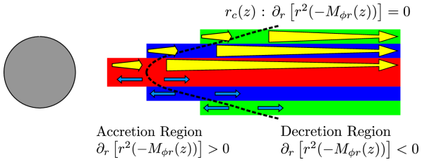
Figure 1.— Structure of a disk dominated by horizontal Maxwell stresses. In each layer, decretion occurs beyond the height-dependent cylindrical radius $r_{c}(z)$, where the radial dependence of the Maxwell stress drops below the critical value $\partial_{r}[r^{2}(-M_{\phi r}(z))]=0$. Blue arrows in the bottom half show the direction of the accretion and decretion flow. For horizontal stresses other than the Maxwell stress, the structure is the same, with the flux and stress replaced as appropriate. Yellow arrows in the top half indicate the outward going Poynting flux, which grows though the accretion region, and deposits energy in the outer, decretion region, although the transition between the growing and shrinking fluxes occurs at $9r_{b}(z)/4$, which need not be the same as $r_{c}(z)$ and defines an alternate critical surface.

As we have reviewed above, in steady state viscous disk models, the vertically integrated radial mass flux is directed inwards while the midplane flow is directed outwards. This occurs because the much stronger radial gradients found at high altitudes drive fast inward flows that overwhelm the midplane’s slower outward flows. Horizontal stresses drive horizontal energy fluxes (Sect. 3.1). Because the mass and energy fluxes are horizontal, this leads to a picture of accretion disks as made up of layered, nearly horizontal slabs rather than adjacent annuli (see Figure 1). In this picture, each individual layer at a height $z$ above the midplane has its own critical radius $r_{c}(z)$ that defines the boundary between accretion and decretion. In a vertically isothermal disk in hydrostatic equilibrium, the density is

$$\rho(r,z)=\rho_{0}(r)e^{-z^{2}/2H^{2}(r)},$$ (32)

where $\rho_{0}$ is the midplane density and $H$ the scale height. Taking the radial derivative we find

$$\partial_{r}\ln\rho(r,z)=\partial_{r}\ln\rho_{0}+\frac{z^{2}}{H^{2}(r)}\partial_{r}\ln H(r).$$ (33)

The density, then, can only be taken to be a power-law in $r$ if the term capturing the radial dependence on $H$ is negligible compared to the radial dependence on the midplane density, which requires $z^{2}/H^{2}\ll 1$. As noted in Section 2.4, disk models with stresses strictly proportional to pressure predict decretion where the disk can behave in a scale-free, power law manner, i.e. where the radial dependence on H in Equation (33) can be neglected. This implies that for each height $z$, the critical radius separating accretion and decretion will be near the radius $r_{pl}(z)$ outside of which the disk, at the height $z$, can be approximated as a powerlaw in radius. While the precise location of $r_{pl}$ will depend on the details of the disk, Equation (33) gives the constraint $H(r_{pl}(z))>z$.

Further, standard viscous disk theory (Frank et al., 2002) for vertically integrated disks invokes another critical radius $r_{b}$ at which $\partial_{r}\varOmega=0$. Outside of

$$r>\frac{9}{4}r_{b}$$ (34)

viscous accretion flows locally dissipate more energy than provided by the accretion power. However, while vertical hydrostatic equilibrium can mathematically be extended to infinity, in practice accretion disks will generally be truncated vertically by stellar or disk winds, or the presence of infalling envelope material. It follows that each altitude $z$ has its own $r_{b}(z)$ where $\partial_{r}\varOmega(r,z)=0$. Accordingly, a similar layered picture results from a analysis of viscous disks performed layer-by-layer, as opposed to the more common vertically-integrated approach. We can construct the surface

$$r(z)=\frac{9}{4}r_{b}(z),$$ (35)

noting that it divides an outer region centered on the midplane that is a net consumer of energy from an inner, surface layer that is a net exporter of energy. (Because disks generally increase in height with radius, their upper surfaces are also their inner edges.) The energetics of global disks depend fundamentally on the material in the surface layer defined in Equation (35), because in viscous disk theory the accretion power below that surface at larger radii is inadequate to power the dissipation (Frank et al., 2002).

3.3. Available Accretion Energy

Can accretion at the inner edge of each layer of the disk provide enough energy to drive the outward motions expected further out? The local surface density of the energy released per unit time by accretion in a vertical slab of a Keplerian disk is

$$Q_{acc}=\int_{z}\frac{1}{2}\rho v_{r}r\varOmega^{2}dz,$$ (36)

where the factor of one half accounts for half of the gravitational potential energy being converted into orbital kinetic energy. Azimuthally integrating Equation (36) for a given slab, we find the total power released at a radius $r$ to be

$$\int_{\phi}Q_{acc}2\pi rd\phi = \frac{1}{2}\left(2\pi r\varSigma v_{r}r\varOmega^{2}\right)$$ (37)

$$= \frac{1}{2}\dot{M}r\varOmega^{2}=\frac{1}{2}\dot{M}r_{f}\varOmega_{f}^{2}\left(\frac{r}{r_{f}}\right)^{-2}.$$

where $\dot{M}$ is the accretion rate (so that $\dot{M}<0$ implies decretion), and $r_{f}$ is a fiducial reference position. In Equation (37) $\Sigma$ is the surface density and $v_{r}$ is the density-weighted mean radial velocity of the slab.

Let us divide our slab into two annuli at $r_{f}$, which we choose to be where $v_{r}=0$, such that there is an inner accretion flow $\dot{M}_{1}>0$ with an inner edge at $r_{0}$, and an outer outwards flow $\dot{M}_{2}<0$ out to $r_{1}$, with $r_{1}\gg r_{f}\gg r_{0}$. Then if the flows are to be powered by the accretion, net gravitational energy must be released by the system. The accretion power provided by the inner annulus is

$$P_{in}=\int_{r_{0}}^{r_{f}}\frac{\dot{M}_{1}r_{f}^{3}\varOmega_{f}^{2}r^{-2}}{2}dr=\frac{1}{2}\dot{M}_{1}\varOmega_{f}^{2}\frac{r_{f}^{2}}{r_{0}}(r_{f}-r_{0}),$$ (38)

while the accretion power provided by the outer annulus is (negative because $\dot{M}_{2}<0$)

$$P_{out}=\int_{r_{f}}^{r_{1}}\frac{1}{2}\dot{M}_{2}r_{f}^{3}\varOmega_{f}^{2}r^{-2}dr=\frac{1}{2}\dot{M}_{2}\varOmega_{f}^{2}\frac{r_{f}^{2}}{r_{1}}(r_{1}-r_{f}).$$ (39)

The condition that net gravitational potential energy be released by this flow, allowing for accretion-powered accretion stresses, is then

$$P_{in}+P_{out}>0,$$ (40)

or

$$\left|\frac{\dot{M}_{1}}{\dot{M}_{2}}\right|>\frac{r_{0}}{r_{1}}\left(\frac{r_{1}-r_{f}}{r_{f}-r_{0}}\right)\simeq\frac{r_{0}}{r_{f}},$$ (41)

where the inequality holds for the broad annuli we assume, with $r_{f}/r_{0}\gg 1$ and $r_{1}/r_{f}\gg 1$. Inner annuli accreting at a rate $\dot{M}_{1}$ therefore release adequate energy to drive broad regions of decretion with $|\dot{M}_{2}|\sim\dot{M}_{1}$, although this is only a necessary requirement, and the details of the energy transport also matter.

3.4. Time Scales of Energy Transfer

The divergence of the Poynting (and analogous hydrodynamical energy) fluxes is comparable to the accretion power and can drive broad outflowing regions. Therefore, we need to consider the impact that changes in the Poynting flux, due, for example, to fluctuations or outbursts in the inner disk, will have on the stresses. We can quantify this by following the analysis of BP99. They derived the local steady state rate of energy dissipation into heat (their Eq. 37) starting from the full energy evolution equation:

$$\frac{\partial\phantom{t}}{\partial t}\left(\frac{1}{2}\rho v^{2}+\rho\Phi+\frac{B^{2}}{2\mu_{0}}\right)+\mbox{\boldmath$\nabla$}{}\cdot\mbox{ ${\cal F}$}{}_{E}=-\mbox{ ${\cal Q}$}{}_{e}$$ (42)

(their Eq. 31). To find the steady state rate, they assume that the time derivatives are negligible, thus identifying the divergence of the energy flux with the local energy dissipation rate $\mbox{ ${\cal Q}$}{}_{e}$ (positive $\mbox{ ${\cal Q}$}{}_{e}$ means energy is deposited as heat). Note that the quantity we define as $\mbox{ ${\cal Q}$}{}_{e}$ is the volume density of the energy dissipation; so the variable $Q_{e}$ defined by BP99, the total energy dissipated per unit time per unit surface area, is

$$Q_{e}=\int_{z}dz\mbox{ ${\cal Q}$}{}_{e}.$$ (43)

That is twice the total power that must be radiated from each disk surface element. Note that $Q_{e}$ is the surface power actually dissipated into heat and radiated away, while $Q_{acc}$ was the accretion power surface density.

In the case of accretion flows driven by Maxwell or turbulent Reynolds stresses, the accretion or decretion power is mediated by the energy density of the magnetic field or of the turbulent flows. If there is a mismatch between the local accretion power and the divergence of the energy fluxes, energy must be injected into or extracted from the local magnetic or turbulent energy densities (see Equation 26 for the magnetic case). For a slab, those azimuthally averaged energy surface densities are

$$\langle E_{T}\rangle_{\phi}=\int_{z}dz\left\langle\frac{1}{2}\rho w^{2}+\frac{B^{2}}{2\mu_{0}}\right\rangle_{\phi},$$ (44)

where we recall that the velocity has been decomposed into a mean orbital $\bar{v}$ and a fluctuating $w$.

The terms that survive averaging are related to the stresses: we have $R_{ij}\equiv\rho w_{i}w_{j}$ and $M_{ij}\equiv\mu_{0}^{-1}B_{i}B_{j}$. Accordingly we can write

$$E_{T}=f\Sigma|W_{r\phi}|$$ (45)

where $f>1$ measures the difference between the squared amplitudes of the magnetic and fluctuating velocity fields $B^{2}$ and $w^{2}$ and their horizontal correlators $|B_{\phi}B_{r}|$ and $|w_{\phi}w_{r}|$. The parameter $f$ relates the stresses to an energy density, and so is a relative of the Shakura-Sunyaev $\alpha$. Indeed, Hawley et al. (2011) defined

$$\alpha_{mag}=-2\frac{B_{r}B_{\phi}}{B^{2}},$$ (46)

finding $\alpha_{mag}\sim 0.3$. We can therefore estimate $f^{-1}\sim\alpha_{mag}/2\sim 0.1$ for MRI active disks.

We can find the accretion power surface density in terms of the stresses from Equation (28) of BP99,

$$P_{acc}=\Sigma R\varOmega_{K}^{2}\langle u_{r}\rangle_{\rho}\sim 2g\varOmega\Sigma W_{r\phi}$$ (47)

where we have assumed that $\Sigma R^{2}W_{r\phi}\propto r^{-g}$. We see then that changes in the divergence of the energy fluxes cause changes in the local stresses and hence accretion rates on a time scale

$$\left|\frac{E_{T}}{P_{acc}}\right|=\left|\frac{f}{2g\varOmega}\right|.$$ (48)

It immediately follows that local regions in accretion disks are only buffered against changes in the incoming energy fluxes for orbital to tens of orbital time scales. This means that the locality time scale for disk accretion is only a few dynamical times, far shorter than the global viscous evolution time. This is most clearly the case in decreting regions, where the energy that powers the decretion must come from somewhere, but even in accreting regions, putting energy into or removing energy from the magnetic field or the turbulence will alter the stresses. Note that this time evolution of $E_{T}$ was set to zero in BP99 even when they considered the non-steady state to derive their Equation 46, as we discuss in detail in Sect. 6.

4. The Shearing Box Approximation

The shearing box approximation neglects curvature terms and radial gradients of the hydrostatic disk background distribution of density and temperature. The curvature terms are consistently neglected by taking the horizontal size of the shearing box to be small compared to the radial position $r_{0}$. This flattening of the differential operators allows replacement of the cylindrical coordinate system with a local, Cartesian one. To arrive at a system where shear periodic boundary conditions can be applied in the radial direction, it is also necessary to neglect a disk’s background radial density and temperature gradients. For the hydrostatic equilibrium pressure $P_{h}$ that characterizes the global hydrostatic disk structure, this approximation about some radius $r_{0}$ is

$$P_{h}(r,z)=P_{h}(r_{0},z)+\mathcal{O}\left(\frac{r-r_{0}}{r_{0}}\right)\$$ (49)

(Goldreich & Lynden-Bell, 1965; Umurhan & Regev, 2004; McNally & Pessah, 2014). This approximation has significant consequences a few scale heights $H$ above the midplane, no matter how cold and thin the disk is, because the approximation cannot capture a radially varying $H$. In particular, meridional flows cannot be driven once this approximation has been made.

The shearing box as commonly employed does, however, provide an internally consistent model for a shearing disk-like flow, if not a strictly valid asymptotic approximation to a section of an accretion disk in hydrostatic equilibrium. Given a shearing box, the underlying conservation properties of magnetohydrodynamics are preserved, up to specific effects of work done at the boundaries (Hawley et al., 1995; McNally & Pessah, 2014). As such, the shearing box has and can be used to understand the local dynamics in a shear flow closely analogous to that of a disk. However, the mass flux through a vertical surface drawn in a disk cannot be determined from this shearing box model alone, due to the neglect of the radial derivatives of the background density and temperature structure and the resulting elimination of any meridional flows.

4.1. The Poynting Flux in the Shearing Box

Consider an incompressible ideal unstratified shearing box. where the velocity $\bm{v}$ has been decomposed into ${\bm{\bar{v}}}+\bm{w}$ with the background shear flow $\bm{\bar{v}}=-q\varOmega x{\bm{\hat{e}}_{y}}$, $\bm{w}$ the fluctuation, and $q=3/2$ in the case of Keplerian rotation with $\varOmega\propto r^{-3/2}$. The governing equations are:

$$\partial_{t}\bm{w} +{\bm{\bar{v}}}\cdot\nabla\bm{w}+\bm{w}\cdot\nabla\bm{w}=$$

$$-2\varOmega{\bm{\hat{e}}_{z}}\times\bm{w}+q\varOmega w_{x}{\bm{\hat{e}}_{y}}+\frac{1}{\mu_{0}\rho}(\nabla\times{\bm{B}})\times{\bm{B}},$$ (50)

$$\partial_{t}{\bm{B}} =\nabla\times\left[(\bm{w}+q\varOmega x{\bm{\hat{e}}_{y}})\times{\bm{B}}\right],$$ (51)

with $\nabla\cdot\bm{w}=0$.

An exact solution of these governing equations is

$$\bm{w}(t) =0,$$ (52)

$${\bm{B}}(t) =\sin(k_{z}z)\left({\bm{\hat{e}}_{x}}+q\varOmega t{\bm{\hat{e}}_{y}}\right),$$ (53)

$$\mu_{0}{\bm{J}}(t) =\nabla\times{\bm{B}}(t)=k_{z}\cos(k_{z}z)\left(-q\varOmega t{\bm{\hat{e}}_{x}}+{\bm{\hat{e}}_{y}}\right),$$ (54)

which has zero net magnetic field at all times. The Lorentz force

$$\mbox{\boldmath$F$}{}_{L}={\bm{J}}\times{\bm{B}}=\frac{k_{z}}{\mu_{0}}\sin(k_{z}z)\cos(k_{z}z)\left(1+q^{2}\varOmega^{2}\right){\bm{\hat{e}}_{z}}$$ (55)

merely captures the magnetic pressure. The fluid is incompressible, so no fluid is accelerated, the kinetic energy of the flow does not evolve and no work is done by the flow.

The only time varying energy in the system is magnetic energy, which evolves according to:

$$\frac{\partial}{\partial t}\left(\frac{B^{2}}{2\mu_{0}}\right) =-\nabla\cdot\left[\frac{1}{\mu_{0}}\left(-\mbox{\boldmath$v$}{}\times\mbox{\boldmath$B$}{}+\eta\mbox{\boldmath$J$}{}\right)\times\mbox{\boldmath$B$}{}\right]$$

$$\qquad-\eta\mbox{\boldmath$J$}{}^{2}-(\mbox{\boldmath$J$}{}\times\mbox{\boldmath$B$}{})\cdot\mbox{\boldmath$v$}{}.$$ (56)

In the ideal limit ($\eta=0$), this has the solution

$$\frac{B^{2}(t)}{2\mu_{0}} =\frac{\sin^{2}(k_{z}z)\left(1+q^{2}\varOmega^{2}t^{2}\right)}{2\mu_{0}}\ ,$$ (57)

which can also be obtained directly from Equation 53.

The rate of energy density growth is then

$$\frac{\partial}{\partial t}\frac{B^{2}(t)}{2\mu_{0}} =\frac{1}{\mu_{0}}\sin^{2}(k_{z}z)q^{2}\varOmega^{2}t\ .$$ (58)

No work is done inside the volume, so the energy must be provided by some flux from outside the volume, namely the Poynting flux ${\bm{S}}$.

For this exact solution,

$$S =\frac{1}{\mu_{0}}q\varOmega x\sin^{2}(k_{z}z)\left[-q\varOmega t{\bm{\hat{e}}_{x}}+{\bm{\hat{e}}_{y}}\right]\,.$$ (59)

The Poynting flux deposits energy into the field at the rate

$$-\nabla\cdot\bm{S} =\frac{q^{2}\varOmega^{2}t}{\mu_{0}}\sin^{2}(k_{z}z)\ ,$$ (60)

which is the same rate that the magnetic energy grows (Equation 58).

We reemphasize that the shear does no work in this scenario, as the associated Lorentz forces are directed in the ${\bm{\hat{e}}_{z}}$ direction, perpendicular to the fluid velocity in the ${\bm{\hat{e}}_{y}}$ direction, so the fluid does not encounter any resistance to its movement. Therefore, even though the energy growth rate contains a factor of the shear rate $q\varOmega$ (Equation 58), the role of the shear is limited to setting the field geometry, which yields the Poynting flux (Equations 59 and 60).

4.2. Energy Fluxes in Shearing Boxes

Starting with the ideal MHD energy flux and generalizing BP99 (Eq. 32), one arrives at

$$\mbox{ ${\cal F}$}{}_{E}=\bm{v}\left(\frac{1}{2}\rho v^{2}+\rho\Phi+P\right)+\frac{{\bm{B}}}{\mu_{0}}\times(\bm{v}\times{\bm{B}})-\bm{\sigma^{\prime}}(\bm{v})\cdot\bm{v}$$ (61)

which includes the kinetic energy, potential energy, thermal energy, magnetic energy, and viscous fluxes. We use the same notation as in the previous section, but in addition, $P$ is the thermal pressure and $\Phi$ is the gravitational potential. The viscous stress tensor is

$$\sigma^{\prime}_{ik}(v)=\nu\rho\left(\frac{\partial v_{i}}{\partial x_{k}}+\frac{\partial v_{k}}{\partial x_{i}}-\frac{2}{3}\delta_{ik}\frac{\partial v_{l}}{\partial x_{l}}\right)+\zeta\delta_{ik}\frac{\partial v_{l}}{\partial x_{l}},$$ (62)

where $\nu$ is the viscosity, and $\zeta$ the bulk viscosity (Landau & Lifshitz, 1959).

In a shearing box, the $y$ and $z$ components of $\mbox{ ${\cal F}$}{}_{E}$ are periodic, but the $x$ component is not:

$$\mbox{ ${\cal F}$}{}_{E}\cdot{\bm{\hat{e}}_{x}}= -q\varOmega x\rho w_{x}w_{y}+w_{x}\left(\frac{1}{2}\rho(\bar{v}^{2}+\bm{w}^{2})+\rho\Phi+P\right)$$

$$+q\varOmega x\frac{1}{\mu_{0}}B_{x}B_{y}+\frac{1}{\mu_{0}}w_{x}B^{2}-\frac{1}{\mu_{0}}B_{x}w_{k}B_{k}$$

$$+q\varOmega x\nu\rho\left[\frac{\partial(-q\varOmega x)}{\partial x}\right]+q\varOmega x\sigma^{\prime}_{xy}(\bm{w})$$

$$-w_{y}\nu\rho\left[\frac{\partial(-q\varOmega x)}{\partial x}\right]-w_{i}\sigma^{\prime}_{xi}(\bm{w})$$ (63)

Hence, the divergence of the energy flux contains the terms

$$\nabla\cdot\mbox{ ${\cal F}$}{}_{E}= -q\varOmega\rho w_{x}w_{y}+q\varOmega\frac{1}{\mu_{0}}B_{x}B_{y}-\nu\rho q^{2}\varOmega^{2}+...$$ (64)

This expression is essentially a differential version of equation (8) from Hawley et al. (1995). These are the energy sources that result from the non-periodic nature of the energy flux in the shearing box. Note that in vacuum, kinetic energy fluxes are zero and Poynting fluxes reduce to radiation fluxes. This means that the energy fluxes can have physically motivated boundary conditions when generalized from shearing boxes to global simulations with disks embedded in vacuum.

4.3. Viscosity-driven Energy Flux in the Shearing Box

We can usefully compare shearing boxes behaving viscously due to Maxwell, Reynolds (or even microphysical viscous) stresses to shearing boxes with imposed constant viscosity $\nu$. A viscous shearing box flow with $\bm{w}=0$ also has a non-zero divergence of the energy flux (Lynden-Bell & Pringle, 1974), but this is accompanied by work done against the viscous friction force. To characterize this, it is useful to state the evolution equation for kinetic energy in an incompressible viscous hydrodynamic flow

$$\frac{\partial}{\partial t}\left(\frac{1}{2}\rho v^{2}\right) =-\nabla\cdot\left[\rho\bm{v}\left(\frac{1}{2}v^{2}+\frac{p}{\rho}\right)-\bm{v}\cdot\bm{\sigma^{\prime}}\right]-\sigma^{\prime}_{ik}\frac{\partial v_{i}}{\partial x_{k}}\ .$$ (65)

In the steady $\bm{w}=0$ shearing box flow without Reynolds stresses, this reduces to a balance between the kinetic energy source from the divergence of the kinetic energy flux, and the dissipation of kinetic energy to heat from the work done against viscous friction:

$$-\nabla\cdot\left[-\bm{v}\cdot\bm{\sigma^{\prime}}\right] =\sigma^{\prime}_{ik}\frac{\partial v_{i}}{\partial x_{k}}\ ,$$ (66)

$$-\nabla\cdot\left[-\bm{{\bm{\bar{v}}}}\cdot\bm{\sigma^{\prime}}(\bm{{\bm{\bar{v}}}})\right] =\sigma^{\prime}_{yx}(\bm{{\bm{\bar{v}}}})\frac{\partial{\bm{\bar{v}}}}{\partial x}\ ,$$ (67)

$$-\nu\rho q^{2}\varOmega^{2} =-\nu\rho q^{2}\varOmega^{2}\ .$$ (68)

The dynamics of the energy flux that results from constant viscosity $\nu$ in a shearing box hence differ strongly from that which results from the shearing of magnetic fields. This is because the energy consumed by the shearing of magnetic fields can remain as magnetic energy, increasing the Maxwell stresses and driving further accretion. By contrast, in the viscous case the work done against viscous friction immediately thermalizes any energy left over from the radial energy flux, which includes the accretion or decretion power. The assumption of constant viscosity means that this energy plays no further role in the accretion process. This can be seen by contrasting the magnetic energy evolution (Eq. 56) to the kinetic energy evolution (Eq. 65), where in the kinetic energy case, the source of kinetic energy due to viscosity in the first term is exactly balanced by the final term, which removes this energy to heat at the same time.

5. Simulations of Accretion Disks

5.1. Applicability of Shearing Boxes

Shearing boxes may lead to unrealistic results when used to model local regions in accretion disks controlled by horizontal Maxwell stresses $M_{\phi r}$. This occurs because the Poynting flux into the simulation domain is unphysically set by the boundaries of the simulation domain, with energy being supplied at the boundaries of the periodic volume. In a given domain, the energy in the magnetic field, and hence the magnetic stress itself, depends on the energy supply. Equivalent constraints also apply to horizontal Reynolds stresses and their accompanying hydrodynamic energy fluxes. Our conclusions about $M_{\phi r}$ are, however, primarily based on overall energy considerations, and so do not address the extent to which local turbulent properties can still be addressed by local models.

Other recent work has indeed called that into question, though. One example is that the MRI appears to expand to the artificially constrained box scale (Simon et al., 2012; Yang et al., 2012; Nauman & Blackman, 2014), again arguing that the local treatment must be carefully interpreted. Another example is a comparison by Regev & Umurhan (2008) of the growth of isolated MHD perturbations in the center of a periodic, 2D, shearing box with the growth of the same perturbations in an otherwise identical domain with free-slip, conducting walls on the radial boundary. When the boxes had width $L_{x}=\pi$, such that the radial boundaries were near the initial perturbations, the shearing box generated spurious energy in the box. However, when they moved the radial edges away by increasing the width of the box to $L_{x}=2\pi$, they found much better agreement between the shearing box and the wall-bounded flow. Their interpretation of this phenomenon was that the shearing box walls were adding energy to the perturbations. We interpret this as being due to the implied Poynting flux (Sect. 4.1).

Nonetheless, there is evidence that the small scale behavior of the MRI can be modeled in restricted domains. Sorathia et al. (2012) examined the behavior of MRI in restricted subdomains of a global model, and found that the correlations of the turbulent fluctuations remained similar. Nonmodal analysis of the most energetic structures over finite growth times in a laboratory-like global MRI configuration also suggests that the shearing waves are a dominant feature in that global problem, and are captured well in the local shearing box approximation (Squire & Bhattacharjee, 2014).

5.2. Existing Global Simulations

In general, global simulations could show either accretion or decretion locally at each radius. Further, the boundary conditions can force the flow. Fromang & Nelson (2006) and Fromang et al. (2011) find both accretion and decretion in global models, with accretion at small radii and decretion at larger radii. Additionally, Fromang et al. (2011) searched for and did not detect a meridional circulation in an MRI active disk. They found in this case that the variation of stress is not proportional to the pressure in the vertical direction as would occur in a solution with vertically constant alpha, explaining their lack of detection of the expected circulation.

Suzuki & Inutsuka (2014) performed global simulations with initial net vertical fields. These simulations are especially interesting because they combine net vertical field with a radial temperature gradient that forces vertical shear. Their analysis of radial flows (Suzuki & Inutsuka, 2014, Section 5.4) is consistent with our analysis. Indeed they estimate that accretion occurs in the interior section of their disk, and decretion occurs in the exterior section as we predict.

In these models, where some mass flows outwards and to higher total energy, the flow must be supplied with energy liberated from some other location where accretion occurs, or from the boundaries. Indeed, in each case, such locations exist, consistent with our findings.

5.3. Comparing Local and Global Simulations

Sorathia et al. (2010) compared the flux-stress relation from a global simulation with the results for shearing boxes from Pessah et al. (2007). They found a qualitative agreement, but also a marked discrepancy, which they suggested was due to inadequate resolution in the global simulations. This resolution difficulty was also noted by Hawley et al. (2011) who attempted to derive resolution criteria from shearing boxes for use in global simulations.

From a different angle, Sorathia et al. (2012) compared small sub-subdomains of a small subdomain of a global simulation with each other and with the original subdomain (but did not invoke the shearing sheet approximation). They found that there was general agreement between the sub-volumes, confirming that local simulations with physical boundary conditions can be used to study small scale phenomena below the scale of their subdomain. Overall, our argument is consistent with published numerical simulations.

5.4. Diagnostics

We have noted that shearing boxes are not subject to energy constraints present in accretion disks; and that global simulations of accretion disks may need to contend with locality time scales of a few tens of orbits. This raises the question of how meaningful our arguments are for global simulations: while the locality time scale we find is just a few orbits, this only allows, but does not force, the disk to behave on those time scales. We propose two diagnostics to measure the effect in practice.

Firstly, the outer-disk growth rate of magnetic instabilities such as the MRI will be partially slaved to the inner, faster growing magnetic field. Radial fluxes originating in the rapidly evolving inner disk should increase the outer disk’s MRI growth rate beyond that following from a radially local analysis. There are suggestions of this behavior in the literature (Flock et al., 2010). Secondly, the MRI has strongly time varying stresses (Hawley et al., 1995; Fleming & Stone, 2003; Bodo et al., 2008; Davis et al., 2010; Hawley et al., 2011; Flock et al., 2011; McNally et al., 2014) and we expect the magnetic stresses can be correlated across large radial extents with a modest lag (on order of the orbital timescale). There are tantalizing hints of such behavior: figure 5 of Dzyurkevich et al. (2010) shows the azimuthal magnetic field at $6$ AU being correlated with that at $4$ AU with a lag of only about $100$ years, or about $10$ local orbits. However, the correlations of the stresses across radius and time are far less clear (their figure 9). Further numerical simulations with more focused diagnostics could better quantify these stress correlations.

5.5. Energy Flux Boundary Conditions

If the Poynting flux at the inner edge of the simulation domain is not zero, then it is either being imposed by the boundary conditions or set by the simulation volume itself. Unless the boundary condition for the Poynting flux is somehow physically determined (e.g. by a stellar magnetosphere), the energy made available to the system will not be physically controlled, and may be significantly larger or smaller than the value in a simulation that included the entire disk. If, on the other hand, the Poynting flux is set to zero at a physical location within the accretion disk, then the energy available to the simulation volume will be significantly below the correct value because the accretion energy liberated inside of this location is not being transported any further into the domain. This is the case for the common choice of absorbing boundary conditions, which resistively destroy the magnetic field in buffer zones at the inner and outer edges of the simulation domain, forcing the Poynting flux to zero.

In vacuum, the Poynting flux reduces to the radiative flux, justifying radial boundaries positioned outside the disk with zero Poynting flux boundary conditions. At the outer edge this is reasonable: the evolution time scale is long, and the outer edge of the simulation domain can be put far from the disk, so that the outer edge of the disk will not cross the boundary during the lifetime of the simulation. At the inner edge however, the edge of the computational domain cannot be put arbitrarily far from the disk edge, and the disk evolution time is fast, so the inner edge of the disk will rapidly overrun the boundary. Once that occurs, the appropriate outwards energy flux entering the simulation domain from accreting gas cannot be tracked.

We need therefore to capture the structure of the inner edge of the disk directly. This is possible in simulations that include the surface of the central object, such as black hole accretion simulations with horizon-penetrating coordinates and computational domains that extend inside the horizon (ex: McKinney & Gammie, 2004). For circumstellar systems where the accretion disc extends smoothly to the stellar surface, this surface provides the appropriate location for the inner radial boundary (Armitage, 2002; Steinacker & Papaloizou, 2002). For circumstellar disks around magnetized stars, though, we suggest instead placing the inner boundary at the interface between the disk and the stellar magnetosphere: energy released by matter accreting in the magnetosphere will travel along the stellar magnetic field lines rather than entering the disk. In practice, this means using a conducting porous boundary that allows both mass flow and magnetic flux detachment. Note that this latter requires resolving the boundary layer that will form as the disk magnetic field piles up against the stellar field, as is done for example by Zanni & Ferreira (2013) in two-dimensional models, and Romanova et al. (2012) in three-dimensional models. These models indeed show strong time-variability, which our results suggest may be required to maintain accretion.

An alternative radial magnetic boundary condition may be to bracket the simulation volume with dead zones dominated by non-ideal effects. If the non-ideal effects are adequate to decouple an inner active region of an accretion disk from the outer active region, then the Poynting flux will not be dynamically important in the outer region. However, in stratified disks with active surface layers, this is unlikely to be the case, and recent results have shown that the Hall effect may allow large scale magnetic fields to develop even in dead zones (Lesur et al., 2014; Bai, 2014). Nonetheless, conveniently, simulations using dead-zones as magnetic boundaries can check their self-consistency post-hoc by evaluating the radial Poynting flux in those self-same dead-zones, determining whether or not they are dynamically significant.

6. Extending BP99

In their classic work, BP99 wrote the evolution of the non-thermal energy density in a viscous disk in their Equation (31), reproduced below:

$$\frac{\partial}{\partial t} \left(\frac{1}{2}\rho v^{2}+\rho\Phi+\frac{B^{2}}{8\pi}\right)$$

$$+\mbox{\boldmath$\nabla$}{}\cdot\left[\mbox{\boldmath$v$}{}\left(\frac{1}{2}\rho v^{2}+\rho\Phi+P\right)+\frac{\mbox{\boldmath$B$}{}}{4\pi}\times(\mbox{\boldmath$v$}{}\times\mbox{\boldmath$B$}{})\right]$$

$$=P\mbox{\boldmath$\nabla$}{}\cdot\mbox{\boldmath$v$}{}-\eta_{V}\left(\delta_{i}v_{j}\right)\left(\delta_{i}v_{j}\right)-\frac{\eta_{B}}{4\pi}|\mbox{\boldmath$\nabla$}{}\times\mbox{\boldmath$B$}{}|^{2}\,,$$ (69)

where $\mbox{\boldmath$v$}{}=R\varOmega{\bm{\hat{e}}_{\phi}}+\mbox{\boldmath$u$}{}$ is the complete velocity field, and $\varOmega$ is purely determined by the gravitational potential $\Phi$ (so $u$ includes terms deriving from radial pressure support and does not have a zero average). The square brackets contain the energy flux and Gaussian CGS units are used. In this section we follow the notation of BP99 and use $R$ for the cylindrical radius.

When considering non-steady state cases (and after vertically integrating and averaging) they arrived at their Equation (46) for the energy dissipated into heat per unit surface area per unit time, also reproduced below:

$$-Q_{e}=\Sigma W_{R\phi}\frac{d\varOmega}{d\ln R}\,;$$ (70)

see also our Section 3.4 and Equation (42). In the analysis adopted by BP99, Equation (70) is accurate to leading order. It is instructive to consider the full expression, with terms of all orders retained. In deriving this expression we use the same procedure as in that work, with two exceptions. Firstly, for a given quantity $X$ we average using

$$\langle X\rangle_{\rho} \equiv\frac{1}{2\pi R\Sigma}\int_{-\infty}^{+\infty}\int_{0}^{2\pi}\rho XRd\phi dz\,,$$ (71)

$$\Sigma \equiv\frac{1}{2\pi R}\int_{-\infty}^{+\infty}\int_{0}^{2\pi}\rho Rd\phi dz\,.$$ (72)

Secondly we define a cylindrical part -spherical part decomposition of $\Phi$

$$\Phi=\Phi_{C}(R)+\Phi_{S}(R,Z)\,,\quad\Phi_{S}(R,0)=0\,.$$ (73)

After significant algebra using the simplifications laid out by BP99, but no approximations, we arrive at a version of Equation (70) with all terms retained:

$$-Q_{e}= \Sigma W_{R\phi}\frac{\partial\varOmega}{\partial\ln R}+\mbox{ ${\cal A}$}{}+\mbox{ ${\cal B}$}{}+\mbox{ ${\cal C}$}{}+\mbox{ ${\cal D}$}{}+\mbox{ ${\cal E}$}{}$$ (74)

$$\mbox{ ${\cal A}$}{}= \frac{\partial}{\partial t}\Sigma\left\langle\frac{1}{2}u^{2}+\frac{B^{2}}{8\pi\rho}\right\rangle_{\rho}$$ (75)

$$= \Sigma\frac{\partial}{\partial t}\left\langle\frac{1}{2}u^{2}+\frac{B^{2}}{8\pi\rho}\right\rangle_{\rho}+\left\langle\frac{1}{2}u^{2}+\frac{B^{2}}{8\pi\rho}\right\rangle_{\rho}\frac{\partial}{\partial t}\Sigma$$

$$\mbox{ ${\cal B}$}{}= \frac{\partial}{\partial t}\Sigma R\varOmega\langle u_{\phi}\rangle_{\rho}$$ (76)

$$\mbox{ ${\cal C}$}{}= -\frac{1}{R}\frac{\partial}{\partial R}R\Sigma\left\langle\frac{1}{2}u^{2}u_{R}+\frac{B_{z}^{2}}{4\pi\rho}u_{R}+\frac{B_{R}B_{z}}{4\pi\rho}u_{z}\right.$$

$$\qquad\qquad\qquad\qquad\left.+\frac{B_{\phi}^{2}}{4\pi\rho}u_{R}+\frac{B_{R}B_{\phi}}{4\pi\rho}u_{\phi}\right\rangle_{\rho}$$ (77)

$$\mbox{ ${\cal D}$}{}= -\frac{1}{R}\frac{\partial}{\partial R}R\Sigma\left\langle\frac{P}{\rho}u_{R}\right\rangle_{\rho}$$ (78)

$$\mbox{ ${\cal E}$}{}= \frac{\partial}{\partial t}\Sigma\langle\Phi_{S}\rangle_{\rho}-\frac{1}{R}\frac{\partial}{\partial R}R\Sigma\langle\Phi_{S}u_{R}\rangle_{\rho}\,.$$ (79)

This expression is exact for the averaging as specified by Equation (71), however it can also be taken as an approximation when expressed in terms of the mean flow variables by extending the averaging over an appropriate small radial interval $\Delta R$; these details are discussed in Appendix A.

It is difficult to determine the order at which small perturbed quantities enter the terms on the right-hand side of Equation (74). The perturbed velocity $u$ is no longer asymptotically small once turbulence has saturated; we do not a priori know the value of the ratio of perturbed velocity components $\langle u_{\phi}u_{r}\rangle_{\rho}/\langle u^{2}\rangle_{\rho}$ but it could easily be less than a tenth; and, crucially, we do not know the time and length scales on which values vary.

However, we merely need to argue that effects beyond those captured in Equation (70) can arise. To do that, we continue by adding only the first term ${\cal A}$ to Equation (70). We neglect the second term of ${\cal A}$, proportional to $\partial_{t}\Sigma$, and ${\cal B}$, because we expect the surface density, pressure and hence also $\langle u_{\phi}\rangle_{\rho}$ to vary only slowly in time, on the long, viscous time scale. We can neglect ${\cal C}$ and ${\cal D}$ in favor of ${\cal A}$ if background and fluctuating quantities vary more slowly in space than in time, i.e. if the fluctuating terms vary over length and time scales $\ell$ and $\tau$ such that

$$\frac{\ell}{\tau}\gg u.$$ (80)

Finally, neglecting ${\cal E}$ implies that the disk is thin enough that the spherical component of the potential $\Phi_{S}$ can be neglected.

Under those conditions, we arrive at an approximate form of Equation (74):

$$-Q_{e}\approx\Sigma W_{R\phi}\frac{\partial\varOmega}{\partial\ln R}+\Sigma\frac{\partial}{\partial t}\left\langle\frac{1}{2}u^{2}+\frac{B^{2}}{8\pi\rho}\right\rangle_{\rho}.$$ (81)

We further recall from Equation (44) that the energy in those reservoirs is related to the stress $W_{R\phi}$. Hence, the energy density in the rightmost term of Equation (81) can be estimated as $f\Sigma W_{R\phi}$ by invoking Equation (45). Neglecting the rightmost term of Equation (81) therefore amounts to neglecting the time derivative of the stresses. The term is however vital if considering physical processes such as the linear growth phase of MRI, where the stresses grow on a timescale $\sim\varOmega^{-1}$.

It is further important because in Section 3.4 we argued that the energy contained in $E_{T}$ can only sustain the power $Q_{e}$ for a few orbits. That means that a significant change in the incoming energy fluxes must change $E_{T}$ on a time scale of only a few times $\varOmega^{-1}$. As a result, the two terms on the right-hand side of Equation (81) are of the same order, and the rightmost term must be kept if time variation in the stresses is contemplated. Future numerical experiments correlating stresses at different radii in global models will be needed to move beyond these order-of magnitude estimates and determine the actual speed of propagation of changes in the energy fluxes, and hence stresses. To diagnose the energetics, the various terms of Equation (74) can be individually tracked in numerical simulations.

7. Conclusions

It has been recognized since the work of Lynden-Bell & Pringle (1974) that large swathes of disks that accrete through horizontal stresses, including by mechanisms such as the MRI, do not release adequate gravitational potential energy to power their dynamics. This can be seen most clearly in the context of meridional circulation and viscously spreading disks: any parcel of gas flowing away from the central object cannot be releasing gravitational potential energy. Indeed it is only in a narrow inner annulus that the accretion power is greater than the dissipation of energy into heat. In regions where the accretion power is inadequate, the energy evolution equation must be balanced by long distance energy fluxes, such as Poynting flux traveling radially through an MRI active disk, or stellar irradiation powering a thermal instability. Further, the mismatch between the local accretion power and energy dissipation is within an order of magnitude of the total local energy density in the fields generating the stresses, in the case of turbulent or magnetic stresses.

We have described two important consequences for accretion disks whose accretion stresses are powered by the accretion energy itself, including MRI active disks. Firstly, because the outer disk dissipates more energy than it provides, and imports the remainder from the inner disk, the outer disk’s behavior depends on the inner disk’s accretion rate. It follows that the energy flux, produced on the fast, dynamical time scale of the inner disk, must be capable of modulating the stresses, and hence accretion rate even in the outer disk with its slower dynamical time scale. In the case of global disks, this means that dynamics in the outer disk (which in viscous disk models needs to import energy even though it is accreting, when vertically integrated) should depend on the energy provided by the inner disk.

In more practical terms, for numerical simulations this means that energy fluxes through the radial boundaries can be important to first order in setting stresses and accretion rates. This behavior cannot be represented in shearing box simulations, where the box sets its own boundary conditions and hence energy fluxes. Shearing boxes are therefore decoupled from a constraint on the available energy that drives the magnetic and turbulent velocity fields exerting stresses on the disk. In the case where the energy fluxes play major roles, temporal changes in the fluxes should cause any stress-exerting turbulence present to temporarily enter forced-turbulence or decaying-turbulence modes. Even in steady states, the local power deficit means that the forced-turbulence picture may apply.

Secondly, the energy fluxes are large compared with the local energy densities associated with the accretion stresses in the sense that the local energy density can only power horizontal accretion stresses for a few orbits. If the time scale were much longer, for example the global disk evolution time scale, then the importance of the energy fluxes would be mitigated: the time scale for the outer disk to adjust itself to the energy fluxes from the inner disk would be too long to matter. However, because the time scale is short, the outer disk must rapidly adjust to changes in the inner disk, which in turn has short dynamical time scales. This short timescale may help explain observations of time-variable accretion flows in protoplanetary disks such as FUors and EXors (Audard et al., 2014).

In sum, we have demonstrated that understanding and accurately treating long distance energy fluxes in disks is vital in modeling and understanding accretion flows. Changes in the energy fluxes in the outer disk due to changes in the accretion rate in the inner disk impact the amplitude of the outer disk’s stresses on dynamical, rather than viscous, time scales. Additionally, we have suggested how to diagnose these phenomena in numerical simulations. In particular, we suggest both correlating stresses at different radii with time lags to determine the speed with which and the extent to which the stresses in the outer disk depend on the stresses (and hence energy release and energy fluxes) in the inner disk; and tracking the full set of contributions to the local energy dissipation (the terms of Equation 74) and comparing their measured magnitudes to empirically determine which are dominant.

Appendix A Alternative Averaging

To read Equation (74) as an approximation expressed in terms of the mean flow variables one exchanges the averaging of Equation (71) for BP99’s choice of averaging which includes averaging over an appropriate, small, radial interval $\Delta R$ given by:

$$\langle X\rangle_{\rho} \equiv\frac{1}{2\pi\Sigma\Delta R}\int_{-\infty}^{+\infty}\int_{R-\Delta R/2}^{R+\Delta R/2}\int_{0}^{2\pi}\rho Xd\phi dR^{\prime}dz\ ,$$ (A1)

$$\Sigma \equiv\frac{1}{2\pi\Delta R}\int_{-\infty}^{+\infty}\int_{R-\Delta R/2}^{R+\Delta R/2}\int_{0}^{2\pi}\rho d\phi dR^{\prime}dz\,.$$ (A2)

The averaging schemes are very similar, and the resulting expression Equation (74) we arrive at can be read using this averaging as approximation. When replacing the averaging in Equation (74) with the form Equation (A1) the approximations implicitly invoked are of the form

$$\int_{R-\Delta R/2}^{R+\Delta R/2}R^{\prime}XdR^{\prime}\approx R\int_{R-\Delta R/2}^{R+\Delta R/2}XdR^{\prime}\,.$$ (A3)

Thus, the approximation is valid for $\Delta R/R\ll 1$.

References

- Andrews et al. (2010) Andrews, S. M., Wilner, D. J., Hughes, A. M., Qi, C., & Dullemond, C. P. 2010, ApJ, 723, 1241
- Armitage (2002) Armitage, P. J. 2002, MNRAS, 330, 895
- Audard et al. (2014) Audard, M., Ábrahám, P., Dunham, M. M., et al. 2014, ArXiv e-prints, arXiv:1401.3368 [astro-ph.SR]
- Bai (2014) Bai, X.-N. 2014, ApJ, 791, 137
- Balbus (2003) Balbus, S. A. 2003, ARA&A, 41, 555
- Balbus & Hawley (1991) Balbus, S. A., & Hawley, J. F. 1991, ApJ, 376, 214
- Balbus & Hawley (1998) Balbus, S. A., & Hawley, J. F. 1998, Reviews of Modern Physics, 70, 1
- Balbus & Papaloizou (1999) Balbus, S. A., & Papaloizou, J. C. B. 1999, ApJ, 521, 650
- Blackman & Pessah (2009) Blackman, E. G., & Pessah, M. E. 2009, ApJ, 704, L113
- Bodo et al. (2008) Bodo, G., Mignone, A., Cattaneo, F., Rossi, P., & Ferrari, A. 2008, A&A, 487, 1
- Ciesla (2007) Ciesla, F. 2007, Science, 318, 613
- Ciesla (2009) Ciesla, F. 2009, Icarus, 200, 655
- Davis et al. (2010) Davis, S. W., Stone, J. M., & Pessah, M. E. 2010, ApJ, 713, 52
- Dullemond et al. (2007) Dullemond, C. P., Hollenbach, D., Kamp, I., & D’Alessio, P. 2007, Protostars and Planets V, 555
- Dzyurkevich et al. (2010) Dzyurkevich, N., Flock, M., Turner, N. J., Klahr, H., & Henning, T. 2010, A&A, 515, A70
- Fleming & Stone (2003) Fleming, T., & Stone, J. M. 2003, ApJ, 585, 908
- Flock et al. (2010) Flock, M., Dzyurkevich, N., Klahr, H., & Mignone, A. 2010, A&A, 516, A26
- Flock et al. (2011) Flock, M., Dzyurkevich, N., Klahr, H., Turner, N. J., & Henning, T. 2011, ApJ, 735, 122
- Frank et al. (2002) Frank, J., King, A., & Raine, D. J. 2002, Accretion Power in Astrophysics: Third Edition (Cambridge)
- Fromang et al. (2011) Fromang, S., Lyra, W., & Masset, F. 2011, A&A, 534, A107
- Fromang & Nelson (2006) Fromang, S., & Nelson, R. P. 2006, A&A, 457, 343