Search for supersymmetry with razor variables in $\Pp\Pp$ collisions at $\sqrt{s}=7$

Abstract

The razor approach to search for R-parity conserving supersymmetric particles is described in detail. Two analyses are considered: an inclusive search for new heavy particle pairs decaying to final states with at least two jets and missing transverse energy, and a dedicated search for final states with at least one jet originating from a bottom quark. For both the inclusive study and the study requiring a bottom-quark jet, the data are examined in exclusive final states corresponding to all-hadronic, single-lepton, and dilepton events. The study is based on the data set of proton-proton collisions at $\sqrt{s}=7$collected with the CMS detector at the LHC in 2011, corresponding to an integrated luminosity of 4.7. The study consists of a shape analysis performed in the plane of two kinematic variables, denoted $M_{R}$ and $R^{2}$, that correspond to the mass and transverse energy flow, respectively, of pair-produced, heavy, new-physics particles. The data are found to be compatible with the background model, defined by studying event simulations and data control samples. Exclusion limits for squark and gluino production are derived in the context of the constrained minimal supersymmetric standard model (CMSSM) and also for simplified-model spectra (SMS). Within the CMSSM parameter space considered, squark and gluino masses up to 1350are excluded at 95% confidence level, depending on the model parameters. For SMS scenarios, the direct production of pairs of top or bottom squarks is excluded for masses as high as 400.

0.1 Introduction

Extensions of the standard model (SM) with softly broken supersymmetry (SUSY) [1, 2, 3, 4, 5] predict new fundamental particles that are superpartners of the SM particles. Under the assumption of $R$-parity [6] conservation, searches for SUSY particles at the fermilab Tevatron [7, 8] and the CERN LHC [9, 10, 11, 12, 13, 14, 15, 16, 17, 18, 19, 20, 21, 22, 23, 24, 25] have focused on event signatures with energetic hadronic jets and leptons from the decays of pair-produced squarks $\PSq$ and gluinos $\PSg$. Such events frequently have large missing transverse energy () resulting from the stable weakly interacting superpartners, one of which is produced in each of the two decay chains.

In this paper, we present the detailed methodology of an inclusive search for SUSY based on the razor kinematic variables [26, 27]. A summary of the results of this search, based on 4.7of $\Pp\Pp$ collision data at $\sqrt{s}=7$collected with the CMS detector at the LHC, can be found in Ref. [28]. The search is sensitive to the production of pairs of heavy particles, provided that the decays of these particles produce significant . The jets in each event are cast into two disjoint sets, referred to as “megajets”.

The razor variables $M_{R}$ and $R^{2}$, defined in Section 0.2, are calculated from the four-momenta of these megajets event-by-event, and the search is performed by determining the expected distributions of SM processes in the two-dimensional ($M_{R}$, $R^{2}$) razor plane. A critical feature of the razor variables is that they are computed in the approximate center-of-mass frame of the produced superpartner candidates.

The megajets represent the visible part of the decay chain of pair-produced superpartners, each of which decays to one or more visible SM particles and one stable, weakly interacting lightest SUSY particle (LSP), here taken to be the lightest neutralino $\chiz_{1}$. In this framework the reconstructed products of the decay chain of each originally produced superpartner are collected into one megajet. Every topology can then be described kinematically by the simplest example of squark-antisquark production with the direct two-body squark decay $\PSq\to\Pq\chiz_{1}$, denoted a “dijet plus ” final state, to which the razor variables strictly apply.

The strategy and execution of the search is summarized as follows:

1. Events with two reconstructed jets at the hardware-based first level trigger (L1) are processed by a dedicated set of algorithms in the high-level trigger (HLT). From the jets and leptons reconstructed at the HLT level, the razor variables $M_{R}$ and $R^{2}$ are calculated and their values are used to determine whether to retain the event for further offline processing. A looser kinematic requirement is applied for events with electrons or muons, due to the smaller rate of SM background for these processes. The correspondence between the HLT and offline reconstruction procedures allows events of interest to be selected more efficiently than is possible with an inclusive multipurpose trigger.

2. In the offline environment, leptons and jets are reconstructed, and a tagging algorithm is applied to identify those jets likely to have originated from a bottom-quark jet ($\cPqb$ jet).

3. The reconstructed objects in each event are combined into two megajets, which are used to calculate the variables $M_{R}$ and $R^{2}$. Several baseline kinematic requirements are applied to reduce the number of misreconstructed events and to ensure that only regions of the razor plane where the trigger is efficient are selected.

4. Events are assigned to final state “boxes” based on the presence or absence of a reconstructed lepton. This box partitioning scheme allows us to isolate individual SM background processes based on the final-state particle content and kinematic phase space; we are able to measure the yield and the distribution of events in the ($M_{R}$, $R^{2}$) razor plane for different SM backgrounds. Events with at least one tagged $\cPqb$ jet are considered in a parallel analysis focusing on a search for the superpartners of third-generation quarks. In total, we consider 12 mutually exclusive final-state boxes: dielectron events (ELE-ELE), electron-muon events (ELE-MU), dimuon events (MU-MU), single-electron events (ELE), single-muon events (MU), and events with no identified electron or muon (HAD), each inclusive or with a $\cPqb$-tagged jet.

5. For each box we use the low ($M_{R}$, $R^{2}$) region of the razor plane, where negligible signal contributions are expected, to determine the shape and normalization of the various background components. An analytic model constructed from these results is used to predict the SM background over the entire razor plane.

6. The data are compared with the prediction for the background in the sensitive regions of the razor plane and the results are used to constrain the parameter space of SUSY models.

This paper is structured as follows. The definition of the razor variables is given in Section 0.2. The trigger and offline event selection are discussed in Section 0.3. The features of the signal and background kinematic distributions are described in Section 0.4. In Section 0.5 we describe the sources of SM background, and in Section 0.6 the analytic model used to characterize this background in the signal regions. Systematic uncertainties are discussed in Section 0.7. The interpretation of the results is presented in Section 0.8 in terms of exclusion limits on squark and gluino production in the context both of the constrained minimal SUSY model (CMSSM) [29, 30, 31] and for some simplified model spectra (SMS) [32, 33, 34, 35, 36]. Section 0.9 contains a summary. For the CMSSM, exclusion limits are provided as a function of the universal scalar and fermion mass values at the unification scale, respectively denoted $m_{0}$ and $m_{1/2}$. For the SMS, limits are provided in terms of the masses of the produced SUSY partner and the LSP.

0.2 The razor approach

The razor kinematic variables are designed to be sensitive to processes involving the pair-production of two heavy particles, each decaying to an unseen particle plus jets. Such processes include SUSY particle production with various decay chains, the simplest example of which is the pair production of squarks, where each squark decays to a quark and the LSP, with the LSP assumed to be stable and weakly interacting. In processes with two or more undetected energetic final-state particles, it is not possible to fully reconstruct the event kinematics. Event-by-event, one cannot make precise assignments of the reconstructed final-state particles (leptons, jets, and undetected neutrinos and LSPs) to each of the original superpartners produced. For a given event, there is not enough information to determine the mass of the parent particles, the subprocess center-of-mass energy $\sqrt{\hat{s}}$, the center-of-mass frame of the colliding protons, or the rest frame of the decay of either parent particle. As a result, it is challenging to distinguish between SUSY signal events and SM background events with energetic neutrinos, even though the latter involve different topologies and mass scales. It is also challenging to identify events with instrumental sources of that can mimic the signal topology.

The razor approach [26, 27] addresses these challenges through a novel treatment of the event kinematics. The key points of this approach are listed below.

• The visible particles (leptons and jets) are used to define two megajets, each representing the visible part of a parent particle decay. The megajet reconstruction ignores details of the decay chains in favor of obtaining the best correspondence between a signal event candidate and the presumption of a pair-produced heavy particle that undergoes two-body decay.

• Lorentz-boosted reference frames are defined in terms of the megajets. These frames approximate, event-by-event, the center-of-mass frame of the signal subprocess and the rest frames of the decays of the parent particles.The kinematic quantities in these frames can be used to extract the relevant SUSY mass scales.

• The razor variables, $M_{R}$, $M_{\mathrm{T}}^{R}$, and $R\equiv M_{\mathrm{T}}^{R}/M_{R}$, are computed from the megajet four-momenta and the in the event. The $M_{R}$ variable is an estimate of an overall mass scale, which in the limit of massless decay products equals the mass of the heavy parent particle. It contains both longitudinal and transverse information, and its distribution peaks at the true value of the new-physics mass scale. The razor variable $M_{\mathrm{T}}^{R}$ is defined entirely from transverse information: the transverse momenta ($\pt$) of the megajets and the . This variable has a kinematic endpoint at the same underlying mass scale as the $M_{R}$ mean value. The ratio $R$ quantifies the flow of energy in the plane perpendicular to the beam and the partitioning of momentum between visible and invisible particles.

• The shapes of the distributions in the ($M_{R}$, $R^{2}$) plane are described for the SM processes. Razor variable distributions exhibit peaks for most SM backgrounds, as a result of turn-on effects from trigger and selection thresholds as well as of the relevant heavy mass scales for SM processes, namely the top quark mass and the $\PW$ and $\cPZ$ boson masses. However, compared with signals involving heavier particles and new-physics sources of , the SM distributions peak at smaller values of the razor variables. For values of the razor variables above the peaks, the SM background distributions (and also the signal distributions) exhibit exponentially falling behavior in the ($M_{R}$, $R^{2}$) plane. Hence, the asymptotic behavior of the razor variables is determined by a combination of the parton luminosities and the intrinsic sources of . The multijet background from processes described by quantum chromodynamics (QCD), which contains the smallest level of intrinsic amongst the major sources of SM background, has the steepest exponential fall-off. Backgrounds with energetic neutrinos from $\PW/\cPZ$ boson and top-quark production exhibit a slower fall-off and resemble each other closely in the asymptotic regime. Thus, razor signals are characterized by peaks in the ($M_{R}$, $R^{2}$) plane on top of exponentially falling SM background distributions. Any SUSY search based on razor variables is then more similar to a “bump-hunt”, e.g., a search for heavy resonances decaying to two jets [37], than to a traditional SUSY search. This justifies the use of a shape analysis, based on an analytic fit of the background, as described in Section 0.6.

0.2.1 Razor megajet reconstruction

The razor megajets are defined by dividing the reconstructed jets of each event into two partitions. Each partition contains at least one jet. The megajet four-momenta are defined as the sum of the four-momenta of the assigned jets. Of all the possible combinations, the one that minimizes the sum of the squared-invariant-mass values of the two megajets is selected. In simulated event samples, this megajet algorithm is found to be stable against variations in the jet definition and it provides an unbiased description of the visible part of the two decay chains in SUSY signal events. The inclusive nature of the megajets allows an estimate of the SM background in the razor plane.

Reconstructed leptons in the final state can be included as visible objects in the reconstruction of the megajets, or they can be treated as invisible, i.e., as though they are escaping weakly interacting particles [26]. For SM background processes such as $\PW(\ell\cPgn)$+jets, the former choice yields more transversely balanced megajets and lower values of $R$. If the leptons are treated as invisible in these processes, the corresponds to the entire $\PW$ boson $\pt$ value, similar to the case of $\cPZ(\cPgn\cPagn)$+jets events.

0.2.2 Razor variables

To the extent that the reconstructed pair of megajets accurately reflects the visible portion of the underlying parent particle decays, the kinematics of the event are equivalent to that of the pair production of heavy squarks $\PSq_{1}$, $\PSq_{2}$, with $\PSq_{i}\to\cPq_{i}\PSGczDo$, where $\PSGczDo$ denotes the LSP and $\cPq_{i}$ denotes the visible products of the decays as represented by the megajets.

The razor analysis approximates the unknown center-of-mass and parent particle rest frames with a razor frame defined unambiguously from measured quantities in the laboratory frame. Two observables $M_{R}$ and $M_{\mathrm{T}}^{R}$ estimate the heavy mass scale $M_{\Delta}$. Consider the two visible four-momenta written in the rest frame of the respective parent particles:

$$p_{\cPq_{1}} =\left(\frac{m_{\PSq}^{2}+m_{\cPq_{1}}^{2}-m_{\chiz_{1}}^{2}}{2m_{\PSq}},\;\frac{M_{\Delta}}{2}\,\hat{u}_{\cPq_{1}}\right),$$

$$p_{\cPq_{2}} =\left(\frac{m_{\PSq}^{2}+m_{\cPq_{2}}^{2}-m_{\chiz_{1}}^{2}}{2m_{\PSq}},\;\frac{M_{\Delta}}{2}\,\hat{u}_{\cPq_{2}}\right).$$

where $\hat{u}_{\cPq_{i}}$ (${i}=1,2$) is a unit three-vector and $m_{\cPq}{}_{i}$ represents the mass corresponding to the megajet, e.g., the top-quark mass for $\PSQt\to\cPqt\PSGczDo$. Here we have parameterized the magnitude of the three-momenta by the mass scale $M_{\Delta}$, where

$$M_{\Delta}^{2}\equiv\frac{\left[m_{\PSq}^{2}-(m_{\cPq}+m_{\chiz_{1}})^{2}\right]\left[m_{\PSq}^{2}-(m_{\cPq}-m_{\chiz_{1}})^{2}\right]}{m_{\PSq}^{2}}.$$ (1)

In the limit of massless megajets we then have $M_{\Delta}=(m_{\PSq}^{2}-m_{\chiz_{1}}^{2})/m_{\PSq}$ and the four-momenta reduce to

$$p_{\cPq_{1}} =\frac{M_{\Delta}}{2}(1,\;\hat{u}_{\cPq_{1}}),$$

$$p_{\cPq_{2}} =\frac{M_{\Delta}}{2}(1,\;\hat{u}_{\cPq_{2}}).$$

The razor variable $M_{R}$ is defined in terms of the momenta of the two megajets by

$$M_{R}\equiv\sqrt{(\abs{\vec{p}_{\cPq_{1}}}+\abs{\vec{p}_{\cPq_{2}}})^{2}-(p^{\cPq_{1}}_{z}+p^{\cPq_{2}}_{z})^{2}}.$$ (2)

where $\vec{p}_{\cPq_{i}}$ is the momentum of megajet $\cPq_{i}$ (${i}=1,2$) and $p^{\cPq_{i}}_{z}$ is its component along the beam direction.

For massless megajets, $M_{R}$ is invariant under a longitudinal boost. It is always possible to perform a longitudinal boost to a razor frame where $p^{\cPq_{1}}_{z}+p^{\cPq_{2}}_{z}$ vanishes, and $M_{R}$ becomes just the scalar sum of the megajet three-momenta added in quadrature. For heavy particle production near threshold, the three-momenta in this razor frame do not differ significantly from the three-momenta in the actual parent particle rest frames. Thus, for SUSY signal events, $M_{R}$ is an estimator of $M_{\Delta}$, and for simulated samples we find that the distribution of $M_{R}$ indeed peaks around the true value of $M_{\Delta}$. This definition of $M_{R}$ is improved with respect to the one used in Ref. [26], to avoid configurations where the razor frame is unphysical.

The razor observable $M_{\mathrm{T}}^{R}$ is defined as

$$M_{\mathrm{T}}^{R}\equiv\sqrt{\frac{\ETmiss(\pt^{\cPq_{1}}+\pt^{\cPq_{2}})-\VEtmiss{\cdot}(\ptvec^{\,\cPq_{1}}+\ptvec^{\,\cPq_{2}})}{2}},$$ (3)

where $\ptvec^{\,\cPq_{i}}$ is the transverse momentum of megajet ${\cPq_{i}}$ ($i=1,2$) and $\pt^{\cPq_{i}}$ is the corresponding magnitude; similarly, $\VEtmiss$ is the missing transverse momentum in the event and its magnitude.

Given a global estimator $M_{R}$ and a transverse estimator $M_{\mathrm{T}}^{R}$, the razor dimensionless ratio is defined as

$$R\equiv\frac{M_{\mathrm{T}}^{R}}{M_{R}}.$$ (4)

For signal events, $M_{\mathrm{T}}^{R}$ has a maximum value (a kinematic endpoint) at $M_{\Delta}$, so $R$ has a maximum value of approximately one. Thus, together with the shape of $M_{R}$ peaking at $M_{\Delta}$, this behavior is in stark contrast with, for example, QCD multijet background events, whose distributions in both $M_{R}$ and $R^{2}$ fall exponentially. These properties allow us to identify a region of the two-dimensional (2D) razor space where the contributions of the SM background are reduced while those of signal events are enhanced.

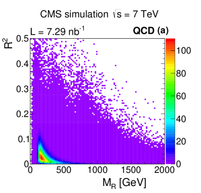
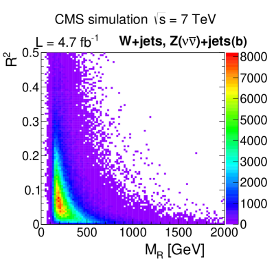
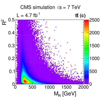
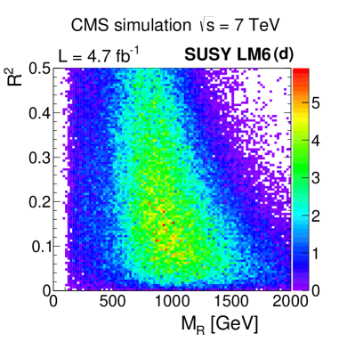
Figure 1: Razor variables $R^{2}$ versus $M_{R}$ for simulated events: (a) QCD multijet, (b) $\PW(\ell\nu)$+jets and $\cPZ(\cPgn\cPagn)$+jets, (c) $\cPqt\cPaqt$, and (d) SUSY benchmark model LM6 [38], where the new-physics mass scale for LM6 is $M_{\Delta}=831$. The yields are normalized to an integrated luminosity of $\sim$4.7 except for the QCD multijet sample, where we use the luminosity of the generated sample. The bin size is 0.005 for $R^{2}$ and 20for $M_{R}$.

0.2.3 SUSY and SM in the razor plane

The expected distributions of the main SM backgrounds in the razor plane, based on simulation, are shown in Fig. 1, along with the results from the CMSSM low-mass benchmark model LM6 [38], for which $M_{\Delta}=831$. The peaking behavior of the signal events at $M_{R}\approx M_{\Delta}$, and the exponential fall-off of the SM distributions with increasing $M_{R}$ and $R^{2}$, are to be noted. For both signal and background processes, events with small values of $M_{R}$ are suppressed because of a requirement that there be at least two jets above a certain threshold in (Section 0.3.5).

In the context of SMS, we refer to the pair production of squark pairs $\PSq$, $\PSq^{*}$, followed by $\PSq\to\Pq~{}\chiz_{1}$, as “T2” scenarios [39], where the $\tilde{\cPq}^{*}$ state is the charge conjugate of the $\tilde{\cPq}$ state. Figure 2 (a) shows a diagram for heavy-squark pair production. The distributions of $M_{R}$ and $R^{2}$ for different LSP masses are shown in Figs. 2 (b) and (c). Figure 2 (d) shows the distribution of signal events in the razor plane. The colored bands running from top left to bottom right show the approximate SM background constant-yield contours. The associated numbers indicate the SM yield suppression relative to the reference line marked “1”. Based on these kinematic properties, a 2D analytical description of the SM processes in the ($M_{R}$, $R^{2}$) plane is developed.

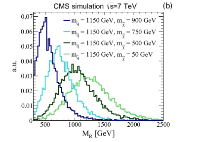
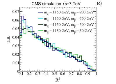
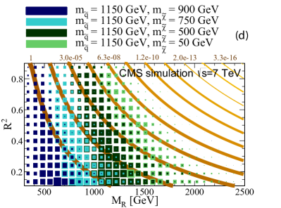
Figure 2: (a) The squark-antisquark production diagram for the T2 SUSY SMS reference model. The distribution of (b) $M_{R}$ and (c) $R^{2}$ for different LSP masses $m_{\tilde{\chi}}$ in the T2 scenario. (d) Distribution of T2 events in the ($M_{R}$, $R^{2}$) plane for the different LSP masses $m_{\tilde{\chi}}$. The orange bands represent contours of constant SM background. The relative suppression factors corresponding to some of the bands are indicated in the upper part of the figure.

0.3 Data taking and event selection

0.3.1 The CMS apparatus

A hallmark of the CMS detector [40] is its superconducting solenoid magnet, of 6 m internal diameter, providing a field of 3.8 T. The silicon pixel and strip tracker, the crystal electromagnetic calorimeter (ECAL), and the brass/scintillator hadron calorimeter (HCAL) are contained within the solenoid. Muons are detected in gas-ionization detectors embedded in the steel flux-return yoke, based on three different technologies: drift tubes, resistive plate chambers, and cathode strip chambers (CSCs). The ECAL has an energy resolution better than 0.5% above 100. The combination of the HCAL and ECAL provides jet energy measurements with a resolution $\Delta E/E\approx 100\%/\sqrt{E/\GeV}\oplus 5\%$.

The CMS experiment uses a coordinate system with the origin located at the nominal collision point, the $x$ axis pointing towards the center of the LHC ring, the $y$ axis pointing up (perpendicular to the plane containing the LHC ring), and the $z$ axis along the counterclockwise beam direction. The azimuthal angle, $\phi$, is measured with respect to the $x$ axis in the $(x,y)$ plane, and the polar angle, $\theta$, is defined with respect to the $z$ axis. The pseudorapidity is $\eta=-\ln[\tan(\theta/2)]$.

For the data used in this analysis, the peak luminosity of the LHC increased from 1$\times 10^{33}$ cm^-2 s^-1 to over 4$\times 10^{33}$ cm^-2 s^-1. For the data collected between (1–2)$\times 10^{33}$ cm^-2 s^-1, the increase was achieved by increasing the number of bunches colliding in the machine, keeping the average number of interactions per crossing at about 7. For the rest of the data, the increase in the instantaneous luminosity was achieved by increasing the number and density of the protons in each bunch, leading to an increase in the average number of interactions per crossing from around 7 to around 17. The presence of multiple interactions per crossing was taken into account in the CMS Monte Carlo (MC) simulation by adding a random number of minimum bias events to the hard interactions, with the multiplicity distribution matching that in data.

0.3.2 Trigger selection

The CMS experiment uses a two-stage trigger system, with events flowing from the L1 trigger at a rate up to 100kHz. These events are then processed by the HLT computer farm. The HLT software selects events for storage and offline analysis at a rate of a few hundred Hz. The HLT algorithms consist of sequences of offline-style reconstruction and filtering modules.

The 2010 CMS razor-based inclusive search for SUSY [26] used triggers based on the scalar sum of jet $\pt$, $\HT$, for hadronic final states and single-lepton triggers for leptonic final states. Because of the higher peak luminosity of the LHC in 2011, the corresponding triggers for 2011 had higher thresholds. To preserve the high sensitivity of the razor analysis, CMS designed a suite of dedicated razor triggers, implemented in the spring of 2011. The total integrated luminosity collected with these triggers was 4.7at $\sqrt{s}=7$.

The razor triggers apply thresholds to the values of $M_{R}$ and $R$ driven by the allocated bandwidth. The algorithms used for the calculation of $M_{R}$ and $R$ are based on calorimetric objects. The reconstruction of these objects is fast enough to satisfy the stringent timing constraints imposed by the HLT.

Three trigger categories are used: hadronic triggers, defined by applying moderate requirements on $M_{R}$ and $R$ for events with at least two jets with $\pt>$ 56; electron triggers, similar to the hadronic triggers, but with looser requirements for $M_{R}$ and $R$ and requiring at least one electron with $\pt>$10satisfying loose isolation criteria; and muon triggers, with similar $M_{R}$ and $R$ requirements and at least one muon with $\abs{\eta}<2.1$ and $\pt>$ 10. All these triggers have an efficiency of $(98\pm 2)\%$ in the kinematic regions used for the offline selection.

In addition, control samples are defined using several non-razor triggers. These include prescaled inclusive hadronic triggers, hadronic multijet triggers, hadronic triggers based on $\HT$, and inclusive electron and muon triggers.

0.3.3 Physics object reconstruction

Events are required to have at least one reconstructed interaction vertex [41]. When multiple vertices are found, the one with the highest scalar sum of charged track $\pt^{2}$ is taken to be the event interaction vertex. Jets are reconstructed offline from calorimeter energy deposits using the infrared-safe anti- [42] algorithm with a distance parameter $R=0.5$. Jets are corrected for the non-uniformity of the calorimeter response in energy and $\eta$ using corrections derived from data and simulations and are required to have $\pt>40$and $\abs{\eta}<3.0$ [43]. To match the trigger requirements, the $\pt$ of the two leading jets is required to be greater than 60. The jet energy scale uncertainty for these corrected jets is 5% [43]. The $\ETmiss$ is defined as the negative of the vector sum of the transverse energies () of all the particles found by the particle-flow algorithm [44].

Electrons are reconstructed using a combination of shower shape information and matching between tracks and electromagnetic clusters [45]. Muons are reconstructed using information from the muon detectors and the silicon tracker and are required to be consistent with the reconstructed primary vertex [46].

The selection criteria for electrons and muons are considered to be tight if the electron or muon candidate is isolated, satisfies the selection requirements of Ref. [47], and lies within $\abs{\eta}<2.5$ and $\abs{\eta}<2.1$, respectively. Loose electron and muon candidates satisfy relaxed isolation requirements.

0.3.4 Selection of good quality data

The 4.7integrated luminosity used in this analysis is certified as having a fully functional detector. Events with various sources of noise in the ECAL or HCAL detectors are rejected using either topological information, such as unphysical charge sharing between neighboring channels, or timing and pulse shape information. The last requirement exploits the difference between the shapes of the pulses that develop from particle energy deposits in the calorimeters and from noise events [48]. Muons produced from proton collisions upstream of the detector (beam halo) can mimic proton-proton collisions with large $\ETm$ and are identified using information obtained from the CSCs. The geometry of the CSCs allows efficient identification of beam halo muons, since halo muons that traverse the calorimetry will mostly also traverse one or both CSC endcaps. Events are rejected if a significant amount of energy is lost in the masked crystals that constitute approximately 1% of the ECAL, using information either from the separate readout of the L1 hardware trigger or by measuring the energy deposited around the masked crystals. We select events with a well-reconstructed primary vertex and with the scalar $\sum\pt$ of tracks associated to it greater than 10% of the scalar $\sum\pt$ of all jet transverse momenta. These requirements reject 0.003% of an otherwise good inclusive sample of proton-proton interactions (minimum bias events).

0.3.5 Event selection and classification

Electrons enter the megajet definition as ordinary jets. Reconstructed muons are not included in the megajet grouping because, unlike electrons, they are distinguished from jets in the HLT. This choice also allows the use of $\PW(\Pgm\cPgn)$+jets events to constrain and study the shape of $\cPZ(\cPgn\cPagn)$+jets events in fully hadronic final states.

The megajets are constructed as the sum of the four-momenta of their constituent objects. After considering all possible partitions into two megajets, the combination is selected that has the smallest sum of megajet squared-invariant-mass values.

The variables $M_{R}$ and $R^{2}$ are calculated from the megajet four-momenta. The events are assigned to one of the six final state boxes according to whether the event has zero, one, or two isolated leptons, and according to the lepton flavor (electrons and muons), as shown in Table 0.3.5. The lepton $\pt$, $M_{R}$, and $R^{2}$ thresholds for each of the boxes are chosen so that the trigger efficiencies are independent of $M_{R}$ and $R^{2}$.

Definition of the full analysis regions for the mutually exclusive boxes, based on the $M_{R}$ and $R^{2}$ values, and, for the categories with leptons, on their value, listed according to the hierarchy followed in the analysis, the ELE-MU (HAD) being the first (last). l c Lepton boxes $M_{R}>300$, $0.11<R^{2}<0.5$
ELE-MU (loose-tight) $\pt>20$, $\pt>15$
MU-MU (loose-loose) $\pt>15$, $\pt>10$
ELE-ELE (loose-tight) $\pt>20$, $\pt>10$
MU (tight) $\pt>12$
ELE (loose) $\pt>20$
HAD box $M_{R}>400$, $0.18<R^{2}<0.5$

The requirements given in Table 0.3.5 determine the full analysis regions of the ($M_{R}$, $R^{2}$) plane for each box. These regions are large enough to allow an accurate characterization of the background, while maintaining efficient triggers. To prevent ambiguities when an event satisfies the selection requirements for more than one box, the boxes are arranged in a predefined hierarchy. Each event is uniquely assigned to the first box whose criteria the event satisfies. Table 0.3.5 shows the box-filling order followed in the analysis.

Six additional boxes are formed with the requirement that at least one of the jets with $\pt>40$and $\abs{\eta}<3.0$ be tagged as a b jet, using an algorithm that orders the tracks in a jet by their impact parameter significance and discriminates using the track with the second-highest significance [49]. This algorithm has a tagging efficiency of about 60%, evaluated using $\cPqb$ jets containing muons from semileptonic decays of $\cPqb$ hadrons in data, and a misidentification rate of about 1% for jets originating from u, d, and s quarks or from gluons, and of about 10% for jets coming from c quarks [49]. The combination of these six boxes defines an inclusive event sample with an enhanced heavy-flavor content.

0.4 Signal and standard model background modeling

The razor analysis is guided by studies of MC event samples generated with the v6.426 [50] (with Z2 tune) and v4.22 [51] programs, using the CTEQ6 parton distribution functions (PDF) [52]. Events generated with are processed with  [50] to provide parton showering, hadronization, and the underlying event description. The matrix element/parton shower matching is performed using the approach described in Ref. [53]. Generated events are processed with the [54] based simulation of the CMS detector, and then reconstructed with the same software used for data.

The simulation of the $\ttbar$, $\PW$+jets, $\cPZ$+jets, single-top ($s$, $t$, and $\cPqt$–$\PW$ channels), and diboson samples is performed using . The events containing top-quark pairs are generated accompanied by up to three extra partons in the matrix-element calculation [55]. Multijet samples from QCD processes are produced using .

To generate SUSY signal MC events in the context of the CMSSM, the mass spectrum is first calculated with the softsusy program [56] and the decays with the sus-hit [57] package. The generator is used with the SUSY Les Houches Accord (SLHA) interface [58] to generate the events. The generator-level cross sections and the K-factors for the next-to-leading-order (NLO) cross sections are computed using prospino [59].

We also use SMS MC simulations in the interpretation of the results. In an SMS simulation, a limited set of hypothetical particles is introduced to produce a given topological signature. The amplitude describing the production and decay of these particles is parameterized in terms of the particle masses. Compared with the constrained SUSY models, SMS provide benchmarks that focus on one final-state topology at a time, with a broader variation in the masses determining the final-state kinematics. The SMS are thus useful for comparing search strategies as well as for identifying challenging areas of parameter space where search methods may lack sensitivity. Furthermore, by providing a tabulation of both the signal acceptance and the 95% confidence level (CL) exclusion limit on the signal cross section as a function of the SMS mass parameters, SMS results can be used to place limits on a wide variety of theoretical models beyond SUSY.

The considered SMS scenarios produce multijet final states with or without leptons and $\cPqb$-tagged jets [39]. While the SUSY terminology is employed, interpretations of SMS scenarios are not restricted to SUSY scenarios.

In the SMS scenarios considered here, each produced particle decays directly to the LSP and SM particles through a two-body or three-body decay. Simplified models that are relevant to inclusive hadronic jets+analyses are gluino pair production with the direct three-body decay $\sGlu\to\cPq\cPaq\chiz_{1}$ (T1), and squark-antisquark production with the direct two-body decay $\sQua\to\cPq\chiz_{1}$ (T2). For $\cPqb$-quark enriched final states, we have considered two additional gluino SMS scenarios, where each gluino is forced into the three-body decay $\sGlu\to\cPqb\cPaqb\chiz_{1}$ with 100% branching fraction (T1bbbb), or where each gluino decays through $\sGlu\to\cPqt\cPaqt\chiz_{1}$ (T1tttt). For $\cPqb$-quark enriched final states we also consider SMS that describe the direct pair production of bottom or top squarks, with the two-body decays $\sBot\to\cPqb\chiz_{1}$ (T2bb) and $\sTop\to\cPqt\chiz_{1}$ (T2tt).

Note that first-generation $\sQua\sQua$ production (unlike $\sQua\sQua^{*}$ production) is not part of the simplified models used for the interpretation of the razor results, even though it is often the dominant process in the CMSSM for low values of the scalar-mass parameter $m_{0}$. This is because of the additional complication that the production rate depends on the gluino mass. However, the acceptance for $\sQua\sQua$ production is expected to be somewhat higher than for $\sQua\sQua^{*}$, so the limits from T2 can be conservatively applied to $\sQua\sQua$ production with analogous decays.

For each SMS, simulated samples are generated for a range of masses of the particles involved, providing a wider spectrum of mass spectra than allowed by the CMSSM. A minimum requirement of ${\cal O}(100~{}\GeV)$ on the mass difference between the mother particle and the LSP is applied, to remove phase space where the jets from superpartner decays become soft and the signal is detected only when it is given a boost by associated jet production. By restricting attention to SMS scenarios with large mass differences, we avoid the region of phase space where accurate modeling of initial- and final-state radiation from quarks and gluons is required, and where the description of the signal shape has large uncertainties.

The production of the primary particles in each SMS is modeled with SUSY processes in the appropriate decoupling limit of the other superpartners. In particular, for $\sQua\,\sQua^{*}$ production, the gluino mass is set to a very large value so that it has a minimal effect on the kinematics of the squarks. The mass spectrum and decay modes of the particles in a specific SMS point are fixed using the SLHA input files, which are processed with v6.426 with Tune Z2 [60, 61] to produce signal events as an input to a parameterized fast simulation of the CMS detector [62], resulting in simulated samples of reconstructed events for each choice of masses for each SMS. These samples are used for the direct calculation of the signal efficiency, and together with the background model are used to determine the 95% CL upper bound on the allowed production cross section.

0.5 Standard model backgrounds in the ($\boldmath{M_{R}}$, $\boldmath{R^{2}}$) razor plane

The distributions of SM background events in both the MC simulations and the data are found to be described by the sum of exponential functions of $M_{R}$ and $R^{2}$ over a large part of the ($M_{R}$, $R^{2}$) plane. Spurious instrumental effects and QCD multijet production are challenging backgrounds due to difficulties in modeling the high $\pt$ and tails. Nevertheless, these event classes populate predictable regions of the ($M_{R}$, $R^{2}$) plane, which allows us to study them and reduce their contribution to negligible levels. The remaining backgrounds in the lepton, dilepton, and hadronic boxes are processes with genuine due to energetic neutrinos and charged leptons from vector boson decay, including $\PW$ bosons from top-quark and diboson production. The analysis uses simulated events to characterize the shapes of the SM background distributions, determine the number of independent parameters needed to describe them, and to extract initial estimates of the values of these parameters. Furthermore, for each of the main SM backgrounds a control data sample is defined using ${\approx}250$of data collected at the beginning of the run. These events cannot be used in the search, as the dedicated razor triggers were not available. Instead, events in this run period were collected using inclusive non-razor hadronic and leptonic triggers, thus defining kinematically unbiased data control samples. We use these control samples to derive a data-driven description of the shapes of the background components and to build a background representation using statistically independent data samples; this is used as an input to a global fit of data selected using the razor triggers in a signal-free region of the ($M_{R}$, $R^{2}$) razor plane.

The two-dimensional probability density function $P_{j}(M_{R},R^{2})$ describing the $R^{2}$ versus $M_{R}$ distribution of each considered SM process $j$ is found to be well approximated by the same family of functions $F_{j}(M_{R},R^{2})$:

$$F_{j}(M_{R},R^{2})=\left[k_{j}(M_{R}-M^{0}_{R,j})(R^{2}-R_{0,j}^{2})-1\right]\times\re^{-k_{j}(M_{R}-M^{0}_{R,j})(R^{2}-R_{0,j}^{2})}.$$ (5)

where $k_{j}$, $M^{0}_{R,j}$, and $R_{0,j}^{2}$ are free parameters of the background model. After applying a baseline selection in the razor kinematic plane, $M_{R}>{M_{R}^{\text{min}}}$ and $R^{2}>{R^{2}_{\text{min}}}$, this function exhibits an exponential behavior in $R^{2}$ ($M_{R}$), when integrated over $M_{R}$ ($R^{2}$):

$$\int_{{R^{2}_{\text{min}}}}^{+\infty}F_{j}(M_{R},R^{2})\rd R^{2} \sim\re^{-(a+b\times{R^{2}_{\text{min}}})M_{R}},$$ (6)

$$\int_{{M_{R}^{\text{min}}}}^{+\infty}F_{j}(M_{R},R^{2})\rd{}M_{R} \sim\re^{-(c+d\times{M_{R}^{\text{min}}})R^{2}},$$ (7)

where $a=-k_{j}\times R_{0,j}^{2}$, $c=-k_{j}\times M^{0}_{R,j}$, and $b=d=k_{j}$. The fact that the function in Eq. (5) depends on $R^{2}$ and not simply on $R$ motivates the choice of $R^{2}$ as the kinematic variable quantifying the transverse imbalance. The values of $M^{0}_{R,j}$, $R_{0,j}$, $k_{j}$, and the normalization constant are floated when fitting the function to the data or simulation samples.

The function of Eq. (5) describes the QCD multijet, the lepton+jets (dominated by $\PW$+jets and events), and the dilepton+jets (dominated by and Z+jets events) backgrounds in the simulation and data control samples. The initial filtering of the SM backgrounds is performed at the trigger level and the analysis proceeds with the analytical description of the SM backgrounds.

0.5.1 QCD multijet background

The QCD multijet control sample for the hadronic box is obtained using events recorded with prescaled jet triggers. The trigger used in this study requires at least two jets with average uncorrected $\pt$ thresholds of 60. The QCD multijet background samples provide $\ga 95\%$ of the events with low $M_{R}$, allowing the study of the $M_{R}$ shapes with different thresholds on $R^{2}$, which we denote ${R^{2}_{\text{min}}}$. The study was repeated using datasets collected with many jet trigger thresholds and prescale factors during the course of the 2011 LHC data taking, with consistent results.

The $M_{R}$ distributions for events satisfying the HAD box selection in this multijet control data sample are shown for different values of the $R_{\text{min}}$ threshold in Fig. 4 (a). The $M_{R}$ distribution is exponentially falling, except for a turn-on at low $M_{R}$ resulting from the $\pt$ threshold requirement on the jets entering the megajet calculation. The exponential region of these distributions is fitted for each value of ${R^{2}_{\text{min}}}$ to extract the absolute value of the coefficient in the exponent, denoted $S$. The value of $S$ that maximizes the likelihood in the exponential fit is found to be a linear function of ${R^{2}_{\text{min}}}$, as shown in Fig 4 (b). Fitting $S$ to the form $S=-a-b{R^{2}_{\text{min}}}$ determines the values of $a$ and $b$.

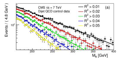
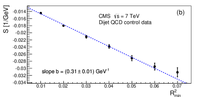
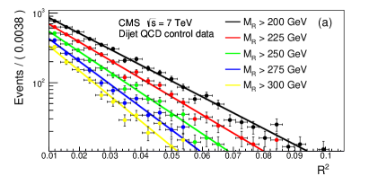
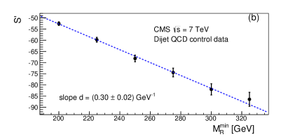
Figure 3: (a) The $M_{R}$ distribution for different values of $R^{2}_{\text{min}}$ for events in the HAD box of a multijet control sample, fit to an exponential function. (b) The coefficient in the exponent $S$ from fits to the $M_{R}$ distributions, as a function of $R^{2}_{\text{min}}$.

Figure 4: (a) The $R^{2}$ distributions for different values of ${M_{R}^{\text{min}}}$ for events in data selected in the HAD box of a multijet control sample, fit to an exponential function. (b) The coefficient in the exponent $S^{\prime}$ from fits to the $R^{2}$ distributions, as a function of ${M_{R}^{\text{min}}}$.

The $R_{\text{min}}^{2}$ distributions are shown for different values of the $M_{R}$ threshold in Fig. 4 (a). The $R^{2}$ distribution is exponentially falling, except for a turn-on at low $R^{2}$. The exponential region of these distributions is fitted for each value of ${M_{R}^{\text{min}}}$ to extract the absolute value of the coefficient in the exponent, denoted by $S^{\prime}$. The value of $S^{\prime}$ that maximizes the likelihood in the exponential fit is found to be a linear function of ${M_{R}^{\text{min}}}$ as shown in Fig. 4 (b). Fitting $S^{\prime}$ to the form $S^{\prime}=-c-dM^{\text{min}}_{R}$ determines the values of $c$ and $d$. The slope $d$ is found to be equal to the slope $b$ to within a few per cent, as seen from the values of these parameters listed in Figs. 4 (b) and 4 (b), respectively. The equality $d=b$ is essential for building the 2D probability density function that analytically describes the $R^{2}$ versus $M_{R}$ distribution, as it reduces the number of possible 2D functions to the function given in Eq. (5). Note that in Eq. (5) the $k_{j}$ parameters are the $b_{j}$, $d_{j}$ parameters used in the description of the SM backgrounds.

0.5.2 Lepton+jets backgrounds

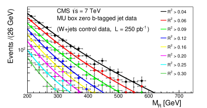
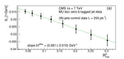
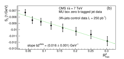
Figure 5: The $M_{R}$ distribution for different values of ${R^{2}_{\text{min}}}$ for events in the MU box, with the requirement of zero $\cPqb$-tagged jets. The curves show the results of fits of a sum of two exponential distributions.

Figure 6: Value of (a) the coefficient in the first exponent, $S_{1}$, and (b) the coefficient in the second exponent, $S_{2}$, from fits to the $M_{R}$ distribution, as a function of ${R^{2}_{\text{min}}}$, for events in the MU box, with the requirement of zero $\cPqb$-tagged jets.

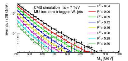
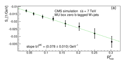
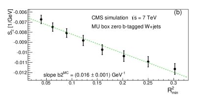
Figure 7: The $M_{R}$ distributions for different values of ${R^{2}_{\text{min}}}$ for $\PW$+jets simulated events in the MU box with the requirement of zero $\cPqb$-tagged jets. The curves show the results of fits of a sum of two exponential distributions.

Figure 8: Value of (a) the coefficient in the first exponent, $S_{1}$, and (b) the coefficient in the second exponent, $S_{2}$, from fits to the $M_{R}$ distribution, as a function of ${R^{2}_{\text{min}}}$, for simulated $\PW$+jets events in the MU box with the requirement of zero $\cPqb$-tagged jets.

The major SM backgrounds with leptons and jets in the final state are ($\PW/\cPZ$)+jets, $\ttbar$, and single-top-quark production. These events can also contain genuine . In both the simulated and the data events in the MU and ELE razor boxes, the $M_{R}$ distribution is well described by the sum of two exponential components. One component, which we denote the “first” component, has a steeper slope than the other, “second” component, i.e., $\abs{S_{1}}>\abs{S_{2}}$, and thus the second component is dominant in the high-$M_{R}$ region. The relative normalization of the two components is considered as an additional degree of freedom. Both the $S_{1}$ and $S_{2}$ values, along with their relative and absolute normalizations, are determined in the fit. The $M_{R}$ distributions are shown as a function of $R_{\text{min}}^{2}$ in Fig. 6 for the zero $\cPqb$-jet MU data, which is dominated by W+jets events. The dependence of $S_{1}$ and $S_{2}$ on $R_{\text{min}}^{2}$ is shown in Fig. 6.

The corresponding results from simulation are shown in Figs. 8 and 8. It is seen that the values of the slope parameters $b_{1}$ and $b_{2}$ from simulation, given in Fig. 8, agree within the uncertainties with the results from data, given in Fig.  6.

The $R^{2}$ distributions as a function of $M_{R}^{\text{min}}$ for the data are shown in Fig. 10 for the MU box with the requirement of zero b-tagged jets. The $S^{\prime}_{1}$ and $S^{\prime}_{2}$ parameters characterizing the exponential behavior of the first and second $\PW(\mu\nu)$+jets components are shown in Fig. 10. The corresponding results from simulation are shown in Figs. 12 and 12. The results for the slopes $d_{1}$ and $d_{2}$ from simulation, listed in Fig. 12, are seen to be in agreement with the measured results, listed in Fig. 10. Furthermore, the extracted values of $d_{1}$ and $d_{2}$ are in agreement with the extracted values of $b_{1}$ and $b_{2}$, respectively. This is the essential ingredient to build a 2D template for the ($M_{R}$,$R^{2}$) distributions, starting with the function of Eq. (5).

The corresponding distributions for the $\ttbar$ MC simulation with $\geq$1 $\cPqb$-tagged jet are presented in Appendix .10, for events selected in the HAD box.

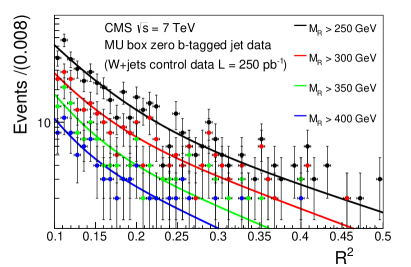
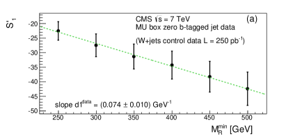
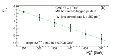
Figure 9: The $R^{2}$ distributions for different values of ${M_{R}^{\text{min}}}$ for events in the MU box, with the requirement of zero $\cPqb$-tagged jets. The curves show the results of fits of a sum of two exponential distributions.

Figure 10: Value of (a) the coefficient in the first exponent, $S^{\prime}_{1}$, and (b) the coefficient in the second exponent, $S^{\prime}_{2}$, from fits to the $R^{2}$ distribution, as a function of ${M_{R}^{\text{min}}}$, for events in the MU box, with the requirement of zero $\cPqb$-tagged jets.

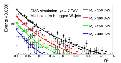
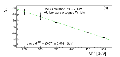
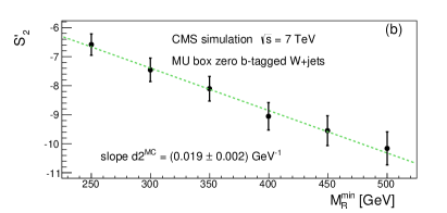
Figure 11: The $R^{2}$ distributions for different values of ${M_{R}^{\text{min}}}$ for $\PW$+jets simulated events in the MU box with the requirement of zero $\cPqb$-tagged jets. The curves show the results of fits of a sum of two exponential distributions.

Figure 12: Value of (a) the coefficient in the first exponent, $S^{\prime}_{1}$, and (b) the coefficient in the second exponent, $S^{\prime}_{2}$, from fits to the $R^{2}$ distribution, as a function of ${M_{R}^{\text{min}}}$, for $\PW$+jets simulated events in the MU box with the requirement of zero $\cPqb$-tagged jets.

0.5.3 Dilepton backgrounds

The SM contributions to the ELE-ELE and MU-MU boxes are expected to be dominated by $\cPZ$+jets events, and the SM contribution to the ELE-MU box by $\ttbar$ events, all at the level of $\ga$95%. We find that the $M_{R}$ distributions as a function of ${R^{2}_{\text{min}}}$, and the $R^{2}$ distribution as a function of ${M_{R}^{\text{min}}}$, are independent of the lepton-flavor combination for both the ELE-ELE and MU-MU boxes, as determined using simulated $\ttbar(2\ell 2\nu$+jets$)$ events. In addition, the asymptotic second component is found to be process-independent.

0.6 Background model and fits

As described earlier, the full 2D SM background representation is built using statistically independent data control samples. The parameters of this model provide the input to the final fit performed in the fit region (FR) of the data samples, defining an extended, unbinned maximum likelihood (ML) fit with the RooFit fitting package [63]. The fit region is defined for each of the razor boxes as the region of low $M_{R}$ and small $R^{2}$, where signal contamination is expected to have negligible impact on the shape fit. The 2D model is extrapolated to the rest of the ($M_{R}$, $R^{2}$) plane, which is sensitive to new-physics signals and where the search is performed.

For each box, the fit is conducted in the signal-free FR of the ($M_{R}$, $R^{2}$) plane; their definition can be found in Figs. 15, 17, 19,  21, 23, and 25. These regions are used to provide a full description of the SM background in the entire ($M_{R}$, $R^{2}$) plane in each box. The likelihood function for a given box is written as [64]:

$$\mathcal{L}_{b}=\frac{\re^{-(\sum_{j\in SM}N_{j})}}{N!}\prod_{i=1}^{N}\left[\sum_{j\in SM}N_{j}P_{j}(M_{R,i},R^{2}_{i})\right],$$ (8)

where $N$ is the total number of events in the FR region of the box, the sum runs over all the SM processes relevant for that box, and the $N_{j}$ are normalization parameters for each SM process involved in the considered box.

We find that each SM process in a given final state box is well described in the ($M_{R}$, $R^{2}$) plane by the function $P_{j}$ defined as

$$P_{j}(M_{R},R^{2})=(1-f^{j}_{2})\times F^{1st}_{j}(M_{R},R^{2})+f^{j}_{2}\times F^{2nd}_{j}(M_{R},R^{2}),$$ (9)

where the first ($F^{1st}_{j}$) and second ($F^{2nd}_{j}$) components are defined as in Eq. (5), and $f^{j}_{2}$ is the normalization fraction of the second component with respect to the total. When fitting this function to the data, the shape parameters of each $F_{j}(M_{R},R^{2})$ function, the absolute normalization, and the relative fraction $f^{j}_{2}$ are floated in the fit. Studies of simulated events and fits to data control samples with either a $\cPqb$-jet requirement or a $\cPqb$-jet veto indicate that the parameters corresponding to the first components of these backgrounds (with steeper slopes at low $M_{R}$ and $R^{2}$) are box-dependent. The parameters describing the second components are box-independent, and at the current precision of the background model, they are identical between the dominant backgrounds considered in these final states.

We validate the choice of the background shape by use of a sample of $\ttbar$ MC simulated events corresponding to an integrated luminosity of 10. Besides being the dominant background in the $\geq$1 $\cPqb$-tag search, $\ttbar$ events are the dominant background for the inclusive search for large values of $M_{R}$ and $R^{2}$. The result for the HAD box in the inclusive razor path is shown in Fig. 13 expressed as the projection of the 2D fit on $M_{R}$ and $R^{2}$. As the same level of agreement is found in all boxes both in the inclusive and in the $\geq$1 $\cPqb$-tagged razor path, we proceed to fit all the SM processes with this shape.

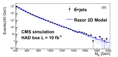
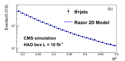
Figure 13: Projection of the 2D fit result on (a) $M_{R}$ and (b) $R^{2}$ for the HAD box in $\ttbar$ MC simulation. The continuous histogram is the 2D model prediction obtained from a single pseudo-experiment based on the 2D fit. The fit is performed in the ($M_{R}$,$R^{2}$) fit region and projected into the full analysis region. Only the statistical uncertainty band in the background prediction is drawn in these projections. The points show the distribution for the MC simulated events.

0.6.1 Fit results and validation

The shape parameters in Eq. (5) are determined for each box via the 2D fit. The likelihood of Eq. (8) is multiplied by Gaussian penalty terms [65] to account for the uncertainties of the shape parameters $k_{j}$, $M^{0}_{R,j}$, and $R_{0,j}^{2}$. The central values of the Gaussians are derived from analogous 2D fits in the low-statistics data control sample. The penalty terms pull the fit to the local minimum closer to the shape derived from the data control samples. Using pseudo-experiments, we verified that this procedure does not bias the determination of the background shape. As an example, the $k_{j}$ parameter uncertainties are typically $\sim$30%. Additional background shape uncertainties due to the choice of the functional form were considered and found to be negligible, as discussed in Appendix .11.

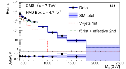
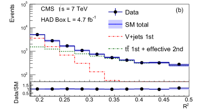
Figure 14: Projection of the 2D fit result on (a) $M_{R}$ and (b) $R^{2}$ for the inclusive HAD box. The continuous histogram is the total SM prediction. The dash-dotted and dashed histograms are described in the text. The fit is performed in the ($M_{R}$, $R^{2}$) fit region (shown in Fig. 15) and projected into the full analysis region. The full uncertainty in the total background prediction is drawn in these projections, including the one due to the variation of the background shape parameters and normalization.

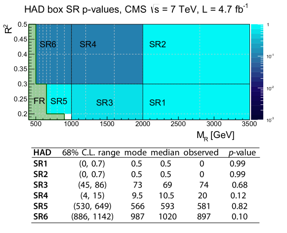
Figure 15: The fit region, FR, and signal regions, SR$i$, are defined in the ($M_{R}$, $R^{2}$) plane for the HAD box. The color scale gives the $p$-values corresponding to the observed number of events in each SR$i$, computed from background parameterization derived in the FR. The $p$-values are also given in the table, together with the observed number of events, the median and the mode of the yield distribution, and a 68% CL interval.

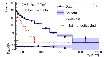
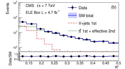
Figure 16: Projection of the 2D fit result on (a) $M_{R}$ and (b) $R^{2}$ for the inclusive ELE box. The fit is performed in the ($M_{R}$, $R^{2}$) fit region (shown in Fig. 17) and projected into the full analysis region. The histograms are described in the text.

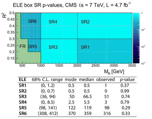
Figure 17: The fit region, FR, and signal regions, SR$i$, are defined in the ($M_{R}$, $R^{2}$) plane for the ELE box. The color scale gives the $p$-values corresponding to the observed number of events in each SR$i$. Further explanation is given in the Fig. 15 caption.

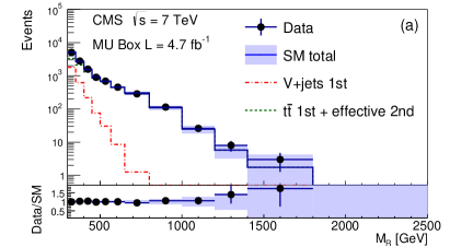
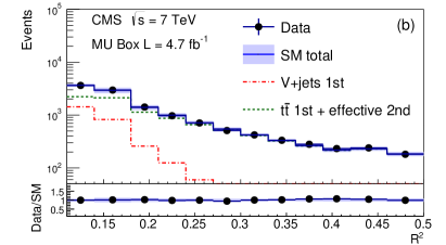
Figure 18: Projection of the 2D fit result on (a) $M_{R}$ and (b) $R^{2}$ for the inclusive MU box. The fit is performed in the ($M_{R}$, $R^{2}$) fit region (shown in Fig. 19) and projected into the full analysis region. The histograms are described in the text.

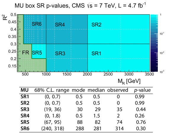
Figure 19: The fit region, FR, and signal regions, SR$i$, are defined in the ($M_{R}$, $R^{2}$) plane for the MU box. The color scale gives the $p$-values corresponding to the observed number of events in each SR$i$. Further explanation is given in the Fig. 15 caption.

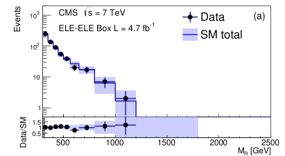
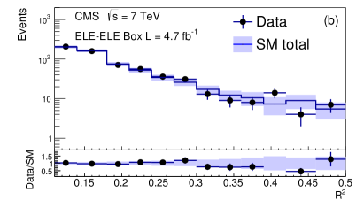
Figure 20: Projection of the 2D fit result on (a) $M_{R}$ and (b) $R^{2}$ for the ELE-ELE box. The continuous histogram is the total standard model prediction. The histogram is described in the text.

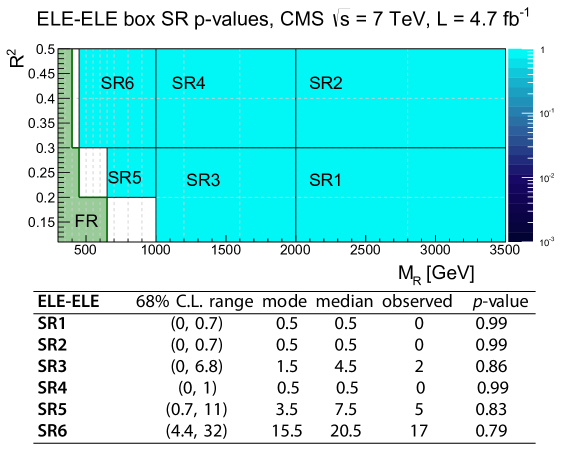
Figure 21: The fit region, FR, and signal regions, SR$i$, are defined in the ($M_{R}$, $R^{2}$) plane for the ELE-ELE box. The color scale gives the $p$-values corresponding to the observed number of events in each SR$i$. Further explanation is given in the Fig. 15 caption.

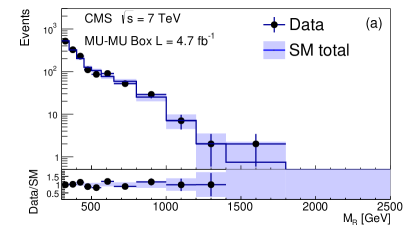
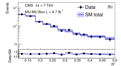
Figure 22: Projection of the 2D fit result on (a) $M_{R}$ and (b) $R^{2}$ for the inclusive MU-MU box. The fit is performed in the ($M_{R}$, $R^{2}$) fit region (shown in Fig. 23) and projected into the full analysis region. The histogram is described in the text.

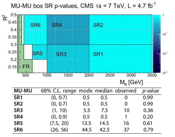
Figure 23: The fit region, FR, and signal regions, SR$i$, are defined in the ($M_{R}$, $R^{2}$) plane for the MU-MU box. The color scale gives the $p$-values corresponding to the observed number of events in each SR$i$. Further explanation is given in the Fig. 15 caption.

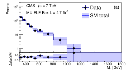
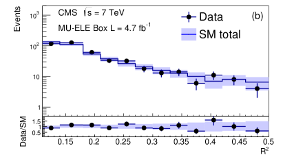
Figure 24: Projection of the 2D fit result on (a) $M_{R}$ and (b) $R^{2}$ for the inclusive MU-ELE box. The fit is performed in the ($M_{R}$, $R^{2}$) fit region (shown in Fig. 25) and projected into the full analysis region. The histogram is described in the text.

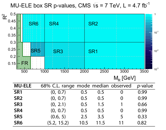
Figure 25: The fit region, FR, and signal regions, SR$i$, are defined in the ($M_{R}$, $R^{2}$) plane for the MU-ELE box. The color scale gives the $p$-values corresponding to the observed number of events in each SR$i$. Further explanation is given in the Fig. 15 caption.

The result of the ML fit projected on $M_{R}$ and $R^{2}$ is shown in Fig. 14 for the inclusive HAD box. No significant discrepancy is observed between the data and the fit model for any of the six boxes. In order to establish the compatibility of the background model with the observed dataset, we define a set of signal regions (SR${i}$) in the tail of the SM background distribution. Using the 2D background model determined using the ML fit, we derive the distribution of the expected yield in each SR${i}$ using pseudo-experiments, accounting for correlations and uncertainties in the parameters describing the background model. In order to correctly account for the uncertainties in the parameters describing the background model and their correlations, the shape parameters used to generate each pseudo-experiment dataset are sampled from the covariance matrix returned by the ML fit performed on the actual dataset. The actual number of events in each dataset is drawn from a Poisson distribution centered on the yield returned by the covariance matrix sampling. For each pseudo-experiment dataset, the number of events in the SR$i$ is found. For each of the SR${i}$, the distribution of the number of events derived by the pseudo-experiments is used to calculate a two-sided $p$-value (as shown for the HAD box in Fig. 15), corresponding to the probability of observing an equal or less probable outcome for a counting experiment in each signal region. The result of the ML fit and the corresponding $p$-values are shown in Figs. 16 and 17 for the ELE box, Figs. 18 and 19 for the MU box, Figs. 20 and 21 for the ELE-ELE box, Figs.22 and 23 for the MU-MU box, and Figs. 24 and 25 for the MU-ELE box. We note that the background shapes in the single-lepton and hadronic boxes are well described by the sum of two functions: a single-component function with a steeper-slope component, denoted as the $\mathrm{V}$+jets first component, obtained by fixing $f_{2}=0$ in Eq. (9); and a two-component function as in Eq. (9), with the first component describing the steeper-slope core of the and single-top background distributions (generically referred to as ), and the effective second component modeling the sum of the indistinguishable tails of different SM background processes. In the dilepton boxes we show the total SM background, which is composed of $\mathrm{V}$+jets and events in the ELE-ELE and MU-MU boxes and of events in the MU-ELE boxes. The corresponding results for the $\geq$1 $\cPqb$-tagged samples are presented in Appendix .12.

0.7 Signal systematic uncertainties

We evaluate the impact of systematic uncertainties on the shape of the signal distributions, for each point of each SUSY model, using the simulated signal event samples. The following systematic uncertainties are considered, with the approximate size of the uncertainty given in parentheses: (i) PDFs (up to 30%, evaluated point-by-point)) [66]; (ii) jet-energy scale (up to 1%, evaluated point-by-point) [43]; (iii) lepton identification, using the “tag-and-probe” technique based on $\cPZ\to\ell\ell$ events [67] ($\ell=\Pe,\mu$, 1% per lepton). In addition, the following uncertainties, which affect the signal yield, are considered: (i) luminosity uncertainty [68] (2.2%); (ii) theoretical cross section [69] (up to 15%, evaluated point-by-point); (iii) razor trigger efficiency (2%); (iv) lepton trigger efficiency (3%). An additional systematic uncertainty is considered for the $\cPqb$-tagging efficiency [49] (between 6% and 20% in $\pt$ bins). We consider variations of the function modeling, the signal uncertainty (log-normal versus Gaussian), and the binning, and find negligible deviations in the results. The systematic uncertainties are included using the best-fit shape to compute the likelihood values for each pseudo-experiment, while sampling the same pseudo-experiment from a different function, derived from the covariance matrix of the fit to the data. This procedure is repeated for both the background and signal probability density functions.

0.8 Interpretation of the results

In order to evaluate exclusion limits for a given SUSY model, its parameters are varied and an excluded cross section at the 95% CL is associated with each configuration of the model parameters, using the hybrid version of the $\mathrm{CL}_{\mathrm{s}}$ method [70, 71, 72], described below.

For each box, we consider the test statistic given by the logarithm of the likelihood ratio $\ln Q=\ln[\mathcal{L}(s+b|H_{i})/\mathcal{L}(b|H_{i})]$, where $H_{i}~{}(i=0,2)$ is the hypothesis under test: $H_{1}$ (signal-plus-background) or $H_{0}$ (background-only). The likelihood function for the background-only hypothesis is given by Eq. (8). The likelihood corresponding to the signal-plus-background hypothesis is written as

$$\mathcal{L}_{s+b}=\frac{\re^{-(\sum_{j\in SM}N_{j})}}{N!}\prod_{i=1}^{N}\left[\sum_{j\in SM}N_{j}P_{j}(M_{R,i},R^{2}_{i})+\sigma\times L\times\epsilon\ P_{S}(M_{R,i},R^{2}_{i})\right],$$ (10)

where $\sigma$ is the signal cross section, , the parameter of interest; $L$ is the integrated luminosity; $\epsilon$ is the signal acceptance times efficiency; and $P_{S}(M_{R,i},R^{2}_{i})$ is the two-dimensional probability density function for the signal, computed numerically from the distribution of simulated signal events. The signal and background shape parameters, and the normalization factors $L$ and $\epsilon$, are the nuisance parameters.

For each analysis (inclusive razor or inclusive $\cPqb$-jet razor) we sum the test statistics of the six corresponding boxes to compute the combined test statistic.

The distribution of $\ln Q$ is derived numerically with a MC technique. The values of the nuisance parameters in the likelihood are randomized for each iteration of the MC generation, to reflect the corresponding uncertainty. Once the likelihood is defined, a sample of events is generated according to the signal and background probability density functions. The value of $\ln Q$ for each generated sample is then evaluated, fixing each signal and background parameter to its expected value. This procedure corresponds to a numerical marginalization of the nuisance parameters.

Given the distribution of $\ln Q$ for the background-only and the signal-plus-background pseudo-experiments, and the value of $\ln Q$ observed in the data, we calculate $\mathrm{CL}_{\mathrm{s+b}}$ and $1-\mathrm{CL}_{\mathrm{b}}$  [70]. From these values, $\mathrm{CL}_{\mathrm{s}}=\mathrm{CL}_{\mathrm{s+b}}/\mathrm{CL}_{\mathrm{b}}$ is computed for that model point. The procedure is independently applied to each of the two analyses (inclusive razor and inclusive $\cPqb$-jet razor).

The CMSSM model is studied in the (${m_{0}}$, $m_{1/2}$) plane, fixing $\tan\beta=10$, $A_{0}=0$, and $\sgn(\mu)=+1$. A point in the plane is excluded at the 95% CL if $\mathrm{CL}_{\mathrm{s}}<0.05$. The result obtained for the inclusive razor analysis is shown in Fig. 26 (a). The shape of the observed exclusion curves reflects the changing relevant SUSY strong-production processes across the parameter space, with squark-antisquark and gluino-gluino production dominating at low and high $m_{0}$, respectively. The observed limit is less constraining than the median expected limit at lower $m_{0}$ due to a local excess of events at large $R^{2}$ in the hadronic box.

For large values of $m_{0}$, boxes with leptons in the final state have a sensitivity comparable to that of the hadronic boxes, as cascade decays of gluinos yield leptons production. Figure 26 parts (b)-(d) show the CMSSM exclusion limits based on the HAD box only and on the leptonic boxes only.

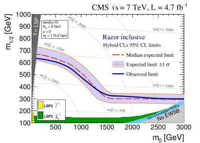
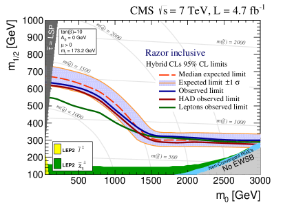
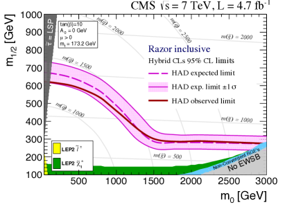
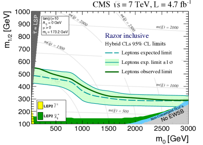
Figure 26: (upper left) Observed (solid curve) and median expected (dashed orange curve) 95% CL limits in the ($m_{0}$, $m_{1/2}$) CMSSM plane (drawn according to Ref. [73]) with $\tan\beta=10$, $A_{0}=0$, and $\sgn(\mu)={+}1$. The ${\pm}$1 standard-deviation equivalent variations due to the uncertainties are shown as a band around the median expected limit. (upper right) The observed HAD-only (solid red) and leptonic-only (solid green) 95% CL limits are shown, compared to the combined limit (solid blue curve). The expected (dashed curve) and observed (solid curve) limits for the (lower left) HAD-only and (lower right) leptonic boxes only are also shown.

The results are also interpreted as cross section limits on a number of simplified models [32, 33, 34, 35, 36] where a limited set of hypothetical particles and decay chains are introduced to produce a given topological signature. For each model studied, we derive the maximum allowed cross section at the 95% CL as a function of the mass of the produced particles (gluinos or squarks, depending on the model) and the LSP mass, as well as the exclusion limit corresponding to the SUSY cross section. We study several SMS benchmark scenarios [39]:

• gluino-gluino production with four light-flavor jets+in the superpartner decays, T1 in Fig. 27.

• squark-antisquark production with two light-flavor jets+in the superpartner decays, T2 in Fig. 27.

• gluino-gluino production with four $\cPqb$ jets+in the superpartner decays, T1bbbb in Fig. 27.

• squark-antisquark production with two $\cPqb$ jets+in the superpartner decays, T2bb in Fig. 27.

• gluino-gluino production with four top quarks+in the superpartner decays, T1tttt in Fig. 27.

• squark-antisquark production with two top quarks+in the superpartner decays, T2tt in Fig. 27.

In all cases, additional jets in the final state can arise from initial- and final-state radiation (ISR and FSR), simulated by . We show in Figs. 28 and  29 the excluded cross section at 95% CL as a function of the mass of the produced particle (gluinos or squarks, depending on the model) and the LSP mass, as well as the exclusion curve corresponding to the NLO+NLL SUSY cross section [74, 75, 76, 77, 78], where NLL indicates the next-to-leading-logarithmic. A result is not quoted for the region of the SMS plane in which the signal efficiency strongly depends on the ISR and FSR modeling (gray area), as a consequence of the small mass difference between the produced superpartner and the LSP and the consequent small for the jets produced in the cascade.

In Fig. 30, we present a summary of the 95% CL excluded largest parent mass for various LSP masses in each of the simplified models studied, showing separately the results from the inclusive razor analysis and the inclusive $\cPqb$-jet razor analysis. A comparison of the razor results with those obtained from other approaches is given in Ref. [79].

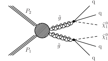
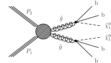
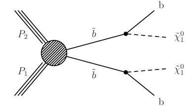
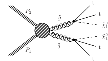
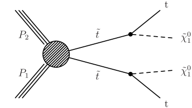
Figure 27: The diagrams corresponding to the SMS models considered in this analysis.

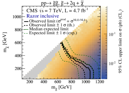
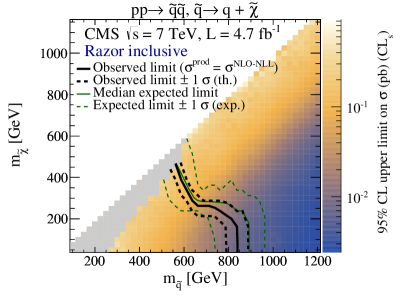
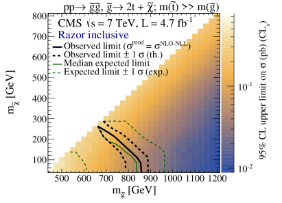
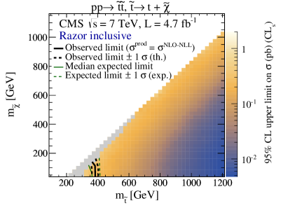
Figure 28: Cross section upper limits, in pb, at 95% CL (color scale), in the mass plane of the produced superparticles for (a) T1, (b) T2, (c) T1tttt, and (d) T2tt, for the inclusive razor analysis. The solid black line indicates the observed exclusion region, assuming the nominal NLO+NLL SUSY production cross section. The dotted black lines show the observed exclusion taking ${\pm}1$ standard deviation theoretical uncertainties around the nominal cross section. The solid green line indicates the median expected exclusion region, with dotted green lines indicating the expected exclusion with ${\pm}1$ standard deviation experimental uncertainties. The solid gray region indicates model points where the selection efficiency is found to have dependence on ISR modeling in the simulation of signal events above a predefined tolerance; no interpretation is presented for these model points.

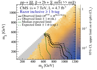
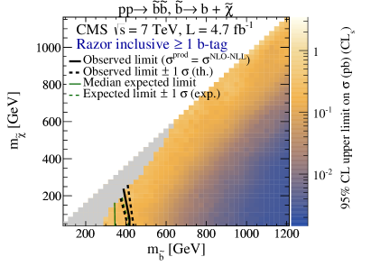
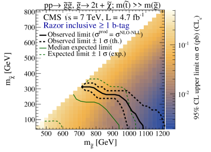
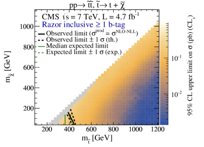
Figure 29: Cross section upper limits, in pb, at 95% CL (color scale), in the mass plane of the produced superparticles for (a) T1bbbb, (b) T2bb, (c) T1tttt, and (d) T2tt, for the $\geq$1 $\cPqb$-tag razor analysis. The solid black line indicates the observed exclusion region, assuming the nominal NLO+NLL SUSY production cross section. The dotted black lines show the observed exclusion taking ${\pm}1$ standard deviation theoretical uncertainties around the nominal cross section. The solid green line indicates the median expected exclusion region, with the dotted green lines indicating the expected exclusion with ${\pm}1$ standard deviation experimental uncertainties. The solid gray region indicates model points where the selection efficiency is found to have dependence on ISR modeling in the simulation of signal events above a predefined tolerance; no interpretation is presented for these model points.

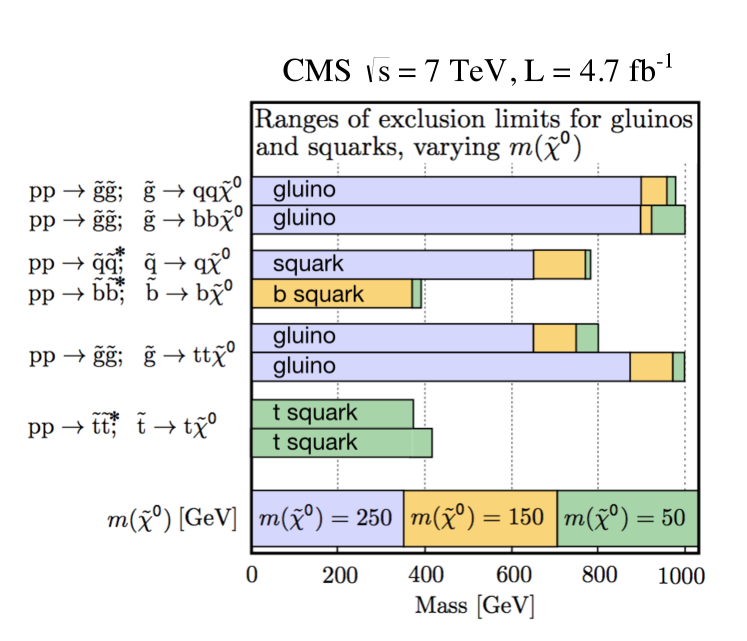
Figure 30: Summary of the 95% CL excluded largest parent mass for each of the simplified models studied, for various LSP masses. The results from the $\cPqb$-jet razor analysis are shown immediately below those from the inclusive razor analysis for each of the four categories of events indicated.

0.9 Summary

Using a data sample of $\sqrt{s}$ = 7proton-proton collisions collected by the CMS experiment at the LHC in 2011, corresponding to an integrated luminosity of 4.7, we have performed a search for pair-produced supersymmetric particles such as squarks and gluinos in the razor-variable plane. A 2D shape description of the relevant standard model processes determined from data control samples and validated with simulated events has been used, and no significant excess over the background expectations has been observed. The results are presented as a 95% CL limit in the ($m_{0}$, $m_{1/2}$) CMSSM parameter space. We exclude squark and gluino masses up to 1350for $m(\PSq)\sim m(\PSg)$, while for $m(\PSq)>m(\PSg)$ we exclude gluino masses up to 800. For simplified models, we exclude gluino masses up to 1000, and first- and second- generation squark masses up to 800. The direct production of top or bottom squarks is excluded for squark masses up to 400.

Appendices

.10 Additional standard model backgrounds in the ($\boldmath{M_{R}}$, $\boldmath{R^{2}}$) razor plane

Figure 32 shows the $M_{R}$ distribution as a function of ${R^{2}_{\text{min}}}$ for $\ttbar$ MC events with $\geq$1 $\cPqb$-tagged jets in the HAD box. The $S_{1}$ and $S_{2}$ parameters characterizing the exponential behavior of the first and second $\PW(\mu\nu)$+jets components are shown in Fig. 32. The corresponding distributions for $R^{2}$, and for the $S^{\prime}_{1}$ and $S^{\prime}_{2}$ parameters, are shown in Figs. 34 and 34, respectively. The conclusions derived from the data and MC studies of Section 0.5 hold also for $\ttbar$ MC events .

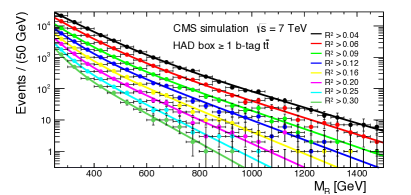
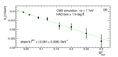
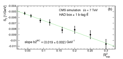
Figure 31: The $M_{R}$ distributions for different values of ${R^{2}_{\text{min}}}$ for $\ttbar$ simulated events in the HAD box with the requirement of $\geq$1 $\cPqb$-tagged jets. The curves show the results of fits of a sum of two exponential distributions.

Figure 32: Value of (a) the coefficient in the first exponent, $S_{1}$, and (b) the coefficient in the second exponent, $S_{2}$, from fits to the $M_{R}$ distribution, as a function of ${R^{2}_{\text{min}}}$, for $\ttbar$ simulated events in the HAD box with the requirement of $\geq$1 $\cPqb$-tagged jets.

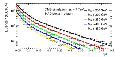
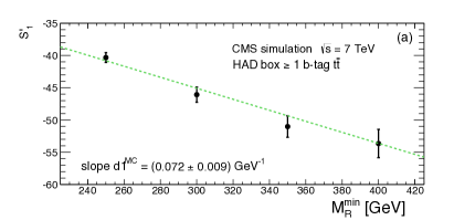
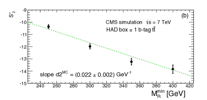
Figure 33: The $R^{2}$ distributions for different values of ${M_{R}^{\text{min}}}$ for $\ttbar$ simulated events in the HAD box with the requirement of $\geq$1 $\cPqb$-tagged jets. The curves show the results of fits of a sum of two exponential distributions.

Figure 34: Value of (a) the coefficient in the first exponent, $S^{\prime}_{1}$, and (b) the coefficient in the second exponent, $S^{\prime}_{2}$, from fits to the $R^{2}$ distribution, as a function of ${M_{R}^{\text{min}}}$, for $\ttbar$ simulated events in the HAD box with the requirement of $\geq$1 $\cPqb$-tagged jets.

.11 Alternative background shape analysis

In order to quantify a systematic uncertainty associated with the choice of the fit function, we first generalize our 2D function to allow for deviations from the exponential behavior, once projected onto $M_{R}$ or $R^{2}$. To do this, we i) identify a set of functions that describe the data, ii) use one as a default description, iii) use the rest to quantify the systematic variation, iv) randomly choose one of the three functions when generating the pseudo-experiments used to set limits, and v) use the nominal function when evaluating the likelihood.

For a 1D fit of the $M_{R}$ distribution, an obvious choice is

$$(M_{R})=A\re^{-bM_{R}^{\beta}},$$ (11)

where $\beta\neq 1$ accounts for deviations from the exponential function. In this analysis, we need a 2D function of $M_{R}$ and $R^{2}$ that allows us to measure the deviation from the nominal shape on the projections. For this purpose, we introduce a generalization of the razor 2D function:

$$F_{\mathrm{SYS}}(M_{R},R^{2})=\left[b(M_{R}-M^{0}_{R})^{1/n}(R^{2}-R_{0}^{2})^{1/n}-n\right]\times\re^{-b(M_{R}-M^{0}_{R})^{1/n}(R^{2}-R_{0}^{2})^{1/n}},$$ (12)

which has the two following properties:

$$\int_{{R^{2}_{\text{min}}}}^{+\infty}F_{\mathrm{SYS}}(M_{R},R^{2})\,\rd R^{2} \sim\re^{-k_{M_{R}}(M_{R}-M_{R}^{0})^{1/n}},$$ (13)

$$\int_{{M_{R}^{\text{min}}}}^{+\infty}F_{\mathrm{SYS}}(M_{R},R^{2})\,\rd M_{R} \sim\re^{-k_{R^{2}}(R^{2}-R^{2}_{0})^{1/n}},$$ (14)

where

$$k_{M_{R}} =(k^{0}_{M_{R}}+b{R^{2}_{\text{min}}})^{1/n},$$ (15)

$$k_{R^{2}} =(k^{0}_{R^{2}}+b{M_{R}^{\text{min}}})^{1/n},$$ (16)

with ${M_{R}^{\text{min}}}$ and ${R^{2}_{\text{min}}}$ respectively the thresholds applied on $M_{R}$ and $R^{2}$ before projecting onto $R^{2}$ and $M_{R}$. Using this function to evaluate systematic uncertainties corresponds to the 2D generalization needed here. We proceed as follows:

• we repeat the fit in the fit region of each box, using $F_{\mathrm{SYS}}(M_{R},R^{2})$ rather than $F(M_{R},R^{2})$ for the second component of the background model (the one that extrapolates to the signal region), with $n$ floated in the fit. We determine $n_{\text{fit}}\pm\sigma_{n}$ in this fit.

• we assign an allowed range to the difference $n-1$ taking the larger of $n_{\text{fit}}-1$ and $\sigma_{n}$, which we refer to as $[n_{\text{min}},n_{\text{max}}]$.

• we repeat the fit in the fit region fixing $n$ to first to $n_{\text{min}}$ and then to $n_{\text{max}}$ and we take these fits as the alternative background descriptions.

In particular, we find that the fit returns values of $n_{\text{fit}}$ that are very close to $n$. Following the prescription outlined above, we take the fit uncertainty as the shift in $n$.

The main conclusion of the study is that the systematic uncertainty in the choice of the function is already covered by the large uncertainty in the fit parameters and that the effect corresponds to an increase of about 15% in the 68% CL range, once this contribution is summed in quadrature with the already quoted uncertainty.

As an example, we present the results of the above procedure for the bins in the HAD box. Fig. 35 shows the fit result with $n$ floated in the full region of the HAD box, projected onto $M_{R}$ and $R^{2}$. The quality of the fit is similar to that of the nominal procedure. We find $n=0.96\pm 0.04$. We then take $n_{\text{min}}=0.96$ and $n_{\text{max}}=1.04$. We show in Table .11 the bin-by-bin background prediction for the nominal fit and the two alternative fits. We use a finer binning than the one used to compute the $p$-values in the nominal analysis. For comparison, we also show the values obtained with $n$ floated in the fit. For all cases, we quote the predicted background as the center of the 68% probability range and the associated uncertainty corresponds to half the range. The range is defined by integrating the background distribution (derived from the pseudo-experiments) using the probability value as the ordering algorithm. Similar results are obtained for all boxes.

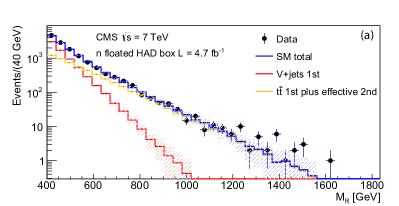
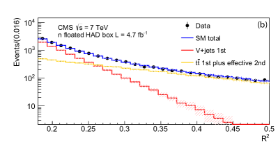
Figure 35: Projection of the fit result on the (a) $M_{R}$ and (b) $R^{2}$ axis for the HAD box, obtained as explained in the text.

The bin-by-bin background prediction for the nominal fit, the two alternative fits, and with $n$ floated, for the HAD box. lxxxx Bin & $n=1$ $n=n_{\text{min}}$ $n=n_{\text{max}}$ $n$ floated
HAD_1_1 1558,69 1527,109 1509,111 1511,126
HAD_1_2 2898,80 2888,89 2868,98 2866,99
HAD_1_3 711,35 729,45 714,43 726,49
HAD_1_4 329,37 338,31 328,32 337,34
HAD_2_1 1785,64 1787,75 1759,69 1774,67
HAD_2_2 3301,82 3336,104 3313,112 3349,118
HAD_2_3 945,46 957,47 957,47 964,48
HAD_2_4 432,36 423,35 454,37 424,38
HAD_3_1 251,26 263,28 259,31 260,29
HAD_3_2 537,47 544,45 561,50 550,49
HAD_3_3 173,36 157,29 182,33 162,34
HAD_3_4 58,18 52,17 66,19 51,18
HAD_4_1 39,9 37,11 43,9 38,9
HAD_4_2 86,23 74,17 90,24 76,21
HAD_4_3 20,7 14,6 22,9 14,7
HAD_4_4 4.2,2.9 2.7,2.3 4.9,3.1 2.4,2.4
HAD_5_1 4.7,2.8 3.9,2.5 5.3,3.1 4.1,2.9
HAD_5_2 8.3,4.7 6.0,3.7 9.5,4.7 5.9,4.0
HAD_5_3 1.2,1.2 0.8,0.8 1.5,1.5 0.8,0.8
HAD_5_4 0.4,0.4 0.4,0.4 0.5,0.5 0.4,0.4
HAD_6_1 0.8,0.8 0.6,0.6 0.9,0.9 0.6,0.6
HAD_6_2 1.0,1.0 0.7,0.7 1.2,1.2 0.8,0.8
HAD_6_3 0.4,0.4 0.3,0.3 0.4,0.4 0.4,0.4

.12 Fit results and validations for $\geq$1 $\cPqb$-tagged events

Figures 36-47 show the results for the $\geq$1 $\cPqb$-tagged jet analysis corresponding to the results presented in Section 0.6.1 for the inclusive analysis.

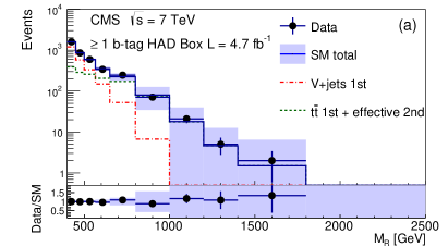
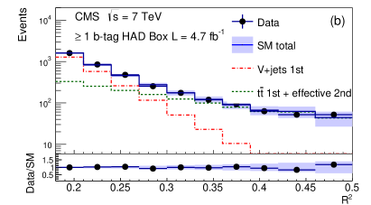
Figure 36: Projection of the 2D fit result on (a) $M_{R}$ and (b) $R^{2}$ for the HAD box in the $\geq$1 $\cPqb$-tag analysis path.

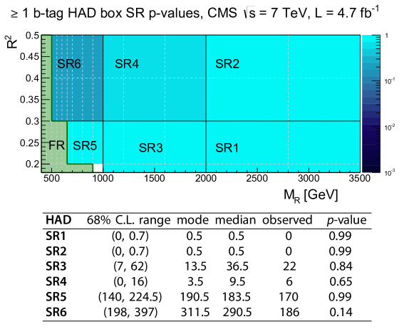
Figure 37: The $p$-values corresponding to the observed number of events in the $\geq$1 $\cPqb$-tag HAD box signal regions (SR$i$).

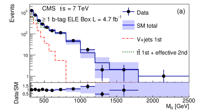
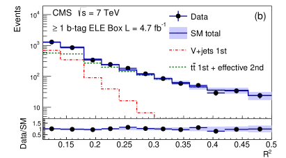
Figure 38: Projection of the 2D fit result on (a) $M_{R}$ and (b) $R^{2}$ for the ELE box in the $\geq$1 $\cPqb$-tag analysis path.

Figure 39: The $p$-values corresponding to the observed number of events in the $\geq$1 $\cPqb$-tag ELE box signal regions (SR$i$).

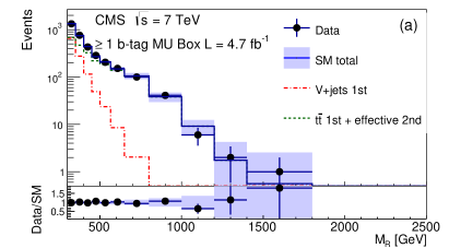
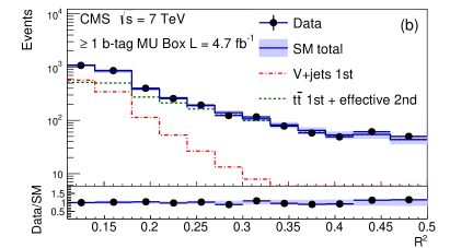
Figure 40: Projection of the 2D fit result on (a) $M_{R}$ and (b) $R^{2}$ for the MU box in the $\geq$1 $\cPqb$-tag analysis path.

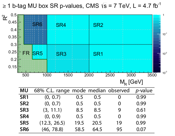
Figure 41: The $p$-values corresponding to the observed number of events in the $\geq$1 $\cPqb$-tag MU box signal regions (SR$i$).

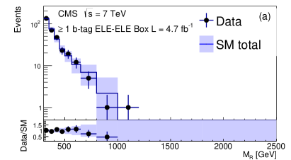
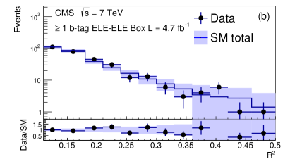
Figure 42: Projection of the 2D fit result on (a) $M_{R}$ and (b) $R^{2}$ for the ELE-ELE box in the $\geq$1 $\cPqb$-tag analysis path.

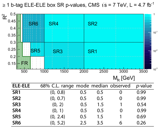
Figure 43: The $p$-values corresponding to the observed number of events in the $\geq$1 $\cPqb$-tag ELE-ELE box signal regions (SR$i$).

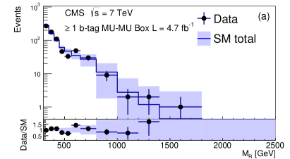
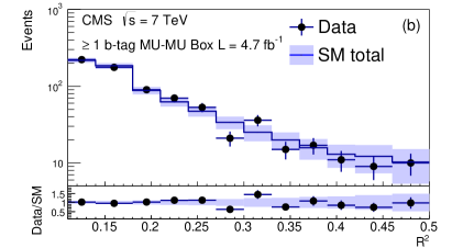
Figure 44: Projection of the 2D fit result on (a) $M_{R}$ and (b) $R^{2}$ for the MU-MU box in the $\geq$1 $\cPqb$-tag analysis path.

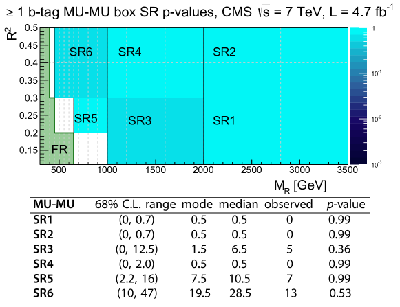
Figure 45: The $p$-values corresponding to the observed number of events in the $\geq$1 $\cPqb$-tag MU-MU box signal regions (SR$i$).

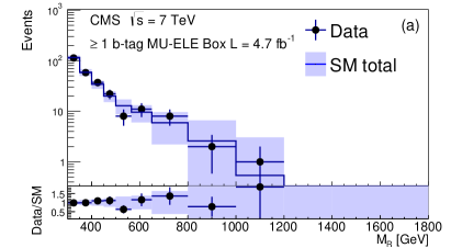
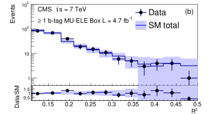
Figure 46: Projection of the 2D fit result on (a) $M_{R}$ and (b) $R^{2}$ for the MU-ELE box in the $\geq$1 $\cPqb$-tag analysis path.

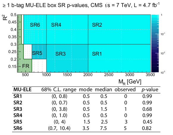
Figure 47: The $p$-values corresponding to the observed number of events in the $\geq$1 $\cPqb$-tag MU-ELE box signal regions (SR$i$).

.13 Guide on emulating the razor analysis for additional studies

In this appendix, we provide a guide to facilitate use of the razor analysis results for the interpretation of signal scenarios not considered here. We assume the existence of an event generator that can simulate LHC collisions for a given theoretical model. We also assume that this event generator is interfaced to a parton shower simulation, such that a list of produced particles at the generator level is available. The procedure described in this appendix represents a simplification of the analysis, giving conservative limits within the $\pm 1$ standard deviation band of the nominal result.

The following classes of stable particles are relevant to this analysis: i) invisible particles (neutrinos and any weakly interacting stable new particles, for example the LSP in SUSY models); ii) electrons; iii) muons; iv) all other stable electrically charged SM particles; and v) all other stable electrically neutral SM particles. It is possible to emulate the razor analysis as follows:

• all the visible stable particles are clustered into generator-level jets using the anti-algorithm with a distance parameter of 0.5.

• the generator-level is computed as $E^{\text{miss}}_{\text{T, Gen}}=-\sum_{p}\pt^{p}$, where the sum runs over all the visible stable particles $p$.

• the detector resolution is applied to electrons and muons according to a simplified Gaussian resolution function. The RMS of the Gaussian smearing depends on the $\eta$ and $\pt$ values of the lepton, as well as its flavor. Similarly, the and jet momenta are smeared according to a Gaussian response model.

• the detector efficiency is applied to electrons and muons generating unweighted events from the reconstruction efficiency, interpreted as a probability (see Section .13.1). The efficiency depends on the $\eta$ and $\pt$ values of the lepton, its flavor, and its generator-level isolation, as computed from the stable particles in the event.

• the analysis selection and box classification is applied.

This procedure allows us to estimate the $R^{2}$ versus $M_{R}$ distribution for a signal model and the efficiency in each box. This is the information that is needed to associate a 95% CL upper limit to a given input model. The procedure matches the full simulation of CMS to within 20% and in general provides a result that is yet closer to the CMS full simulation. The result is in general conservative, since the computation of the upper limit starts from a simplified binned likelihood, which reduces the sensitivity to a signal. This procedure is not expected to correctly simulate the special case of slowly moving electrically charged particles (e.g., staus). The remainder of this appendix describes each step of the razor emulation in more detail, including the calculation of the exclusion limit.

.13.1 Emulation of reconstructed electrons and muons

The emulation of reconstructed electrons and muons consists of two independent steps: the accounting for the detector resolution and for the reconstruction efficiency.

The effects of detector resolution can be incorporated through a Gaussian smearing of the genuine $\pt$ of a given lepton, while the lepton $\eta$ and $\phi$ can be considered to be unaffected by the detector resolution. The generated lepton is then replaced by the reconstructed one, having the same flight direction with a $\pt$ value randomly extracted according to a Gaussian distribution centered at $\pt^{\text{Gen}}$ and with $\sigma(\pt^{\text{Gen}})$ taken from Fig. 48. Any lepton outside the two $\eta$ ranges considered in Fig. 48 should be discarded from the analysis.

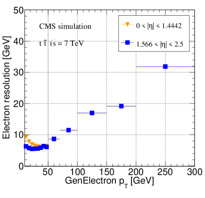
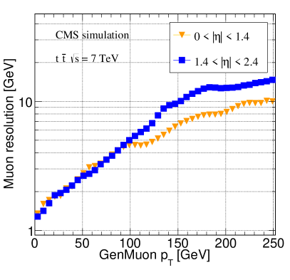
Figure 48: Momentum resolution for (left) electrons and (right) muons within the barrel region of the CMS detector (squares) and in the endcaps (triangles).

To account for the reconstruction efficiency of a given lepton, the generator-level isolation is computed as follows:

$$\text{GenIso}(\ell)=\frac{\sum_{p\neq\ell}\pt^{p}}{\pt^{\ell}},$$ (17)

where the sum runs over all the stable charged and neutral visible particles $p$ within a distance $\Delta R=\sqrt{(\Delta\eta)^{2}+(\Delta\phi)^{2}}<0.5$ from the lepton.

Figure 49 shows the reconstruction probability versus the generated electron $\pt$ (before accounting for the detector resolution) for three ranges of GenIso in the ECAL barrel ($\abs{\eta}<1.4442$) and endcap ($1.5660<\abs{\eta}<2.5000$) regions. Different values are obtained for the tight and the loose electrons used to define the boxes.

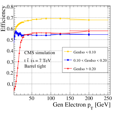
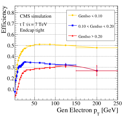
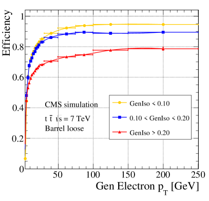
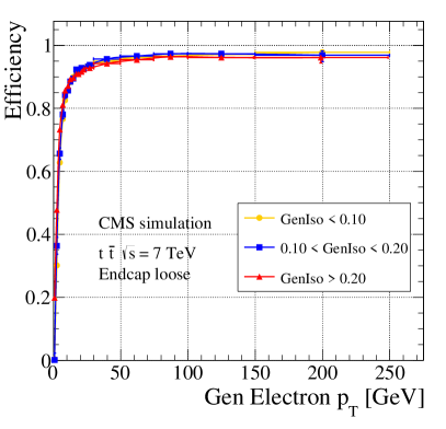
Figure 49: Electron reconstruction efficiency for (top panes) tight and (bottom panes) loose electrons pointing to the ECAL (left panes) barrel and (right panes) endcaps, estimated from the CMS MC simulation of $\cPqt\cPaqt$ events. The electron reconstruction is described in Ref. [45].

Similarly, the reconstruction efficiency for the tight muons is shown in Fig. 50. The reconstruction of loose muons can be considered to be fully efficient for muons with $\pt>10$, since no isolation requirement is applied.

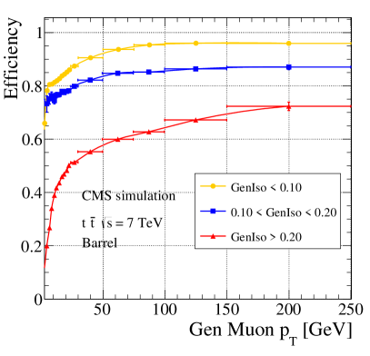
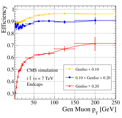
Figure 50: Muon reconstruction efficiency for tight muons pointing to the (left) barrel and (right) endcaps, estimated from the CMS MC simulation of $\ttbar$ events. The muon reconstruction is described in Ref. [46].

Once the lepton reconstruction probability is found, the detector efficiency effects can be imposed numerically: the lepton is rejected if a uniformly distributed random number in the range [0,1] is found to be larger than the reconstruction efficiency.

.13.2 Emulation of reconstructed jets and

The reconstruction of jets and can be emulated by applying a Gaussian resolution to the generator-level quantities. We show in Fig. 51 the dependence of the Gaussian $\sigma_{\text{jet}}$ on the jet $\pt$ (for the two relevant bins of $\eta$) and the . The dependence on $\eta$ or other quantities can be safely neglected. One should apply the resolution function to all the reconstructed jets and to the and then impose the acceptance selection on the reconstructed jets.

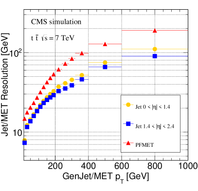
Figure 51: Transverse energy resolution for jets and , in the CMS MC simulation of events.

.13.3 Building the 2D templates

Once detector effects have been accounted for, jets are clustered in two megajets. The razor variables can be computed from the four-momenta of the two megajets.

Figure 52 (left) and (middle) shows the $M_{R}$ and $R^{2}$ distributions for a sample of pair-produced gluinos of mass 800, where each gluino decays to a $\ttbar$ pair and a LSP of mass 300, obtained with the CMS fast simulations program and with the emulation described in this appendix. The efficiencies obtained for the six boxes are compared in Fig. 52 (right).

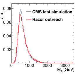
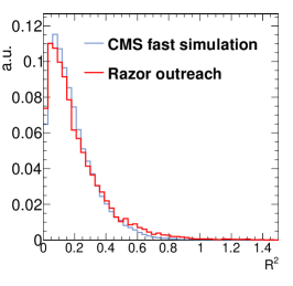
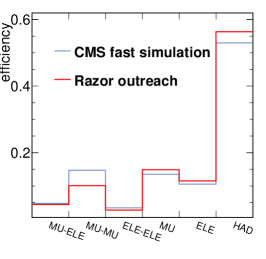
Figure 52: Comparison of the (left) $M_{R}$ distribution, (middle) $R^{2}$ distribution, and (right) the efficiency versus box obtained from the official CMS fast simulation package and the emulation procedure described in this appendix. The two distributions correspond to a T1tttt sample with 800gluino mass and 300LSP mass.

.13.4 Evaluating the exclusion limit

The exclusion limit can be computed from the 2D signal templates and the box efficiencies, starting with the observed yield and the expected background. We consider a simplified likelihood obtained by defining bins in the ($M_{R}$, $R^{2}$) plane. Each bin $i$ requires the observed yield $n_{i}$ and the expected background $\bar{b}_{i}\pm\delta_{i}$ computed by integrating the background model and taking into account the uncertainty in shape. The likelihood in a given box is then written as:

$$\mathcal{L}_{\text{box}}(\vec{n}|\sigma,\vec{b},\rho)=\mathop{\mathrm{log}\mathcal{N}}\nolimits(b_{i}|\bar{b}_{i},\delta_{i})\mathop{\mathrm{log}\mathcal{N}}\nolimits(\rho|1,\delta_{\rho})\textstyle{\prod\nolimits}_{i}P(n_{i}|\epsilon_{i}\rho L\sigma+b_{i}),$$ (18)

where $\epsilon_{i}$ is the signal efficiency in that bin, $L$ is the luminosity, and $\sigma$ is the signal cross section; $\mathop{\mathrm{log}\mathcal{N}}\nolimits(b_{i}|\bar{b}_{i},\delta_{i})$ is the log-normal distribution describing the uncertainty in the background. $\mathop{\mathrm{log}\mathcal{N}}\nolimits(\rho|1,\delta_{\rho})$ is the distribution describing the uncertainty in the signal efficiency. A value $\delta_{\rho}\sim 0.20$ (including the uncertainty in the integrated luminosity) is large enough to account for the use of a simplified detector emulation and the typical systematic uncertainty quoted in the analysis. Once this uncertainty is included, the uncertainty in the luminosity can be neglected to a good level of precision. Similarly, the total likelihood can be written as:

$$\mathcal{L}_{\text{TOT}}(\vec{n}|\sigma,\vec{b},\rho)=\mathop{\mathrm{log}\mathcal{N}}\nolimits(\rho|1,\delta_{\rho})[\textstyle{\prod\nolimits_{\text{box}}}\textstyle{\prod\nolimits_{i}}P(n_{i}^{\text{box}}|\epsilon_{i}^{\text{box}}\rho L\sigma+b_{i}^{\text{box}})\times\mathop{\mathrm{log}\mathcal{N}}\nolimits(b_{i}^{\text{box}}|\bar{b}_{i}^{\text{box}},\delta_{i}^{\text{box}})].$$ (19)

In this case, the signal systematic parameter $\rho$ is common to the six boxes. A Bayesian upper limit (UL) on the cross section can then be computed assuming a flat prior distribution in $\sigma$:

$$\frac{\int_{0}^{\sigma\mathrm{UL}}\rd\sigma\int\rd\rho\,\rd\vec{b}\,\mathcal{L}_{\text{TOT}}(\vec{n}|\sigma,\vec{b},\rho)}{\int_{0}^{+\infty}\rd\sigma\int\rd\rho\,\rd{}\vec{b}\,\mathcal{L}_{\text{TOT}}(\vec{n}|\sigma,\vec{b},\rho)}=0.95.$$ (20)

An implementation of this simplified limit calculator is currently available at [80] together with the values of $n$, $\cPqb$, and $\delta$ for each bin in each box.

.13.5 Limit on simplified models

Figure 53 shows the limit on the T2tt and T1tttt models, obtained by applying the simplified procedure described in this appendix. We generate a sample of SUSY events using the 8 [81] program, scanning the two SMS planes. We then emulate the detector effects as described in this appendix to derive the efficiency and the ($M_{R}$, $R^{2}$) signal probability density functions. We use this information to compute the excluded cross section for each point in the SMS plane.

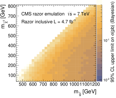
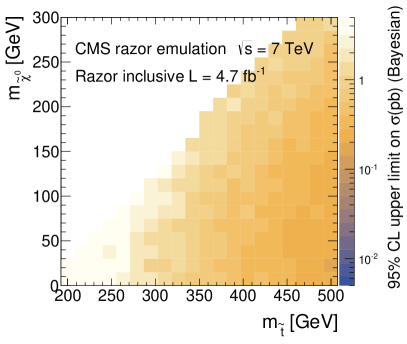
Figure 53: Bayesian upper limits, at 95% CL, on cross sections, in pb, for simplified models, obtained by applying the razor emulation procedure described in this appendix: (left) T1tttt, to be compared with Fig. 28 (c); (right) T2tt, to be compared with Fig. 28 (d).

.14 The CMS Collaboration

Yerevan Physics Institute, Yerevan, Armenia
S. Chatrchyan, V. Khachatryan, A.M. Sirunyan, A. Tumasyan Institut für Hochenergiephysik der OeAW, Wien, Austria
W. Adam, T. Bergauer, M. Dragicevic, J. Erö, C. Fabjan1, M. Friedl, R. Frühwirth1, V.M. Ghete, C. Hartl, N. Hörmann, J. Hrubec, M. Jeitler1, W. Kiesenhofer, V. Knünz, M. Krammer1, I. Krätschmer, D. Liko, I. Mikulec, D. Rabady2, B. Rahbaran, H. Rohringer, R. Schöfbeck, J. Strauss, A. Taurok, W. Treberer-Treberspurg, W. Waltenberger, C.-E. Wulz1 National Centre for Particle and High Energy Physics, Minsk, Belarus
V. Mossolov, N. Shumeiko, J. Suarez Gonzalez Universiteit Antwerpen, Antwerpen, Belgium
S. Alderweireldt, M. Bansal, S. Bansal, T. Cornelis, E.A. De Wolf, X. Janssen, A. Knutsson, S. Luyckx, S. Ochesanu, B. Roland, R. Rougny, H. Van Haevermaet, P. Van Mechelen, N. Van Remortel, A. Van Spilbeeck Vrije Universiteit Brussel, Brussel, Belgium
F. Blekman, S. Blyweert, J. D’Hondt, N. Heracleous, A. Kalogeropoulos, J. Keaveney, T.J. Kim, S. Lowette, M. Maes, A. Olbrechts, Q. Python, D. Strom, S. Tavernier, W. Van Doninck, P. Van Mulders, G.P. Van Onsem, I. Villella Université Libre de Bruxelles, Bruxelles, Belgium
C. Caillol, B. Clerbaux, G. De Lentdecker, L. Favart, A.P.R. Gay, A. Léonard, P.E. Marage, A. Mohammadi, L. Perniè, T. Reis, T. Seva, L. Thomas, C. Vander Velde, P. Vanlaer, J. Wang Ghent University, Ghent, Belgium
V. Adler, K. Beernaert, L. Benucci, A. Cimmino, S. Costantini, S. Crucy, S. Dildick, G. Garcia, B. Klein, J. Lellouch, J. Mccartin, A.A. Ocampo Rios, D. Ryckbosch, S. Salva Diblen, M. Sigamani, N. Strobbe, F. Thyssen, M. Tytgat, S. Walsh, E. Yazgan, N. Zaganidis Université Catholique de Louvain, Louvain-la-Neuve, Belgium
S. Basegmez, C. Beluffi3, G. Bruno, R. Castello, A. Caudron, L. Ceard, G.G. Da Silveira, C. Delaere, T. du Pree, D. Favart, L. Forthomme, A. Giammanco4, J. Hollar, P. Jez, M. Komm, V. Lemaitre, J. Liao, O. Militaru, C. Nuttens, D. Pagano, A. Pin, K. Piotrzkowski, A. Popov5, L. Quertenmont, M. Selvaggi, M. Vidal Marono, J.M. Vizan Garcia Université de Mons, Mons, Belgium
N. Beliy, T. Caebergs, E. Daubie, G.H. Hammad Centro Brasileiro de Pesquisas Fisicas, Rio de Janeiro, Brazil
G.A. Alves, M. Correa Martins Junior, T. Dos Reis Martins, M.E. Pol Universidade do Estado do Rio de Janeiro, Rio de Janeiro, Brazil
W.L. Aldá Júnior, W. Carvalho, J. Chinellato6, A. Custódio, E.M. Da Costa, D. De Jesus Damiao, C. De Oliveira Martins, S. Fonseca De Souza, H. Malbouisson, M. Malek, D. Matos Figueiredo, L. Mundim, H. Nogima, W.L. Prado Da Silva, J. Santaolalla, A. Santoro, A. Sznajder, E.J. Tonelli Manganote6, A. Vilela Pereira Universidade Estadual Paulista ^a,  Universidade Federal do ABC ^b,  São Paulo, Brazil
C.A. Bernardes^b, F.A. Dias^a,7, T.R. Fernandez Perez Tomei^a, E.M. Gregores^b, P.G. Mercadante^b, S.F. Novaes^a, Sandra S. Padula^a Institute for Nuclear Research and Nuclear Energy, Sofia, Bulgaria
V. Genchev2, P. Iaydjiev2, A. Marinov, S. Piperov, M. Rodozov, G. Sultanov, M. Vutova University of Sofia, Sofia, Bulgaria
A. Dimitrov, I. Glushkov, R. Hadjiiska, V. Kozhuharov, L. Litov, B. Pavlov, P. Petkov Institute of High Energy Physics, Beijing, China
J.G. Bian, G.M. Chen, H.S. Chen, M. Chen, R. Du, C.H. Jiang, D. Liang, S. Liang, X. Meng, R. Plestina8, J. Tao, X. Wang, Z. Wang State Key Laboratory of Nuclear Physics and Technology, Peking University, Beijing, China
C. Asawatangtrakuldee, Y. Ban, Y. Guo, Q. Li, W. Li, S. Liu, Y. Mao, S.J. Qian, D. Wang, L. Zhang, W. Zou Universidad de Los Andes, Bogota, Colombia
C. Avila, L.F. Chaparro Sierra, C. Florez, J.P. Gomez, B. Gomez Moreno, J.C. Sanabria Technical University of Split, Split, Croatia
N. Godinovic, D. Lelas, D. Polic, I. Puljak University of Split, Split, Croatia
Z. Antunovic, M. Kovac Institute Rudjer Boskovic, Zagreb, Croatia
V. Brigljevic, K. Kadija, J. Luetic, D. Mekterovic, S. Morovic, L. Tikvica University of Cyprus, Nicosia, Cyprus
A. Attikis, G. Mavromanolakis, J. Mousa, C. Nicolaou, F. Ptochos, P.A. Razis Charles University, Prague, Czech Republic
M. Bodlak, M. Finger, M. Finger Jr. Academy of Scientific Research and Technology of the Arab Republic of Egypt, Egyptian Network of High Energy Physics, Cairo, Egypt
Y. Assran9, S. Elgammal10, A. Ellithi Kamel11, M.A. Mahmoud12, A. Mahrous13, A. Radi10^,14 National Institute of Chemical Physics and Biophysics, Tallinn, Estonia
M. Kadastik, M. Müntel, M. Murumaa, M. Raidal, A. Tiko Department of Physics, University of Helsinki, Helsinki, Finland
P. Eerola, G. Fedi, M. Voutilainen Helsinki Institute of Physics, Helsinki, Finland
J. Härkönen, V. Karimäki, R. Kinnunen, M.J. Kortelainen, T. Lampén, K. Lassila-Perini, S. Lehti, T. Lindén, P. Luukka, T. Mäenpää, T. Peltola, E. Tuominen, J. Tuominiemi, E. Tuovinen, L. Wendland Lappeenranta University of Technology, Lappeenranta, Finland
T. Tuuva DSM/IRFU, CEA/Saclay, Gif-sur-Yvette, France
M. Besancon, F. Couderc, M. Dejardin, D. Denegri, B. Fabbro, J.L. Faure, C. Favaro, F. Ferri, S. Ganjour, A. Givernaud, P. Gras, G. Hamel de Monchenault, P. Jarry, E. Locci, J. Malcles, A. Nayak, J. Rander, A. Rosowsky, M. Titov Laboratoire Leprince-Ringuet, Ecole Polytechnique, IN2P3-CNRS, Palaiseau, France
S. Baffioni, F. Beaudette, P. Busson, C. Charlot, N. Daci, T. Dahms, M. Dalchenko, L. Dobrzynski, N. Filipovic, A. Florent, R. Granier de Cassagnac, L. Mastrolorenzo, P. Miné, C. Mironov, I.N. Naranjo, M. Nguyen, C. Ochando, P. Paganini, D. Sabes, R. Salerno, J.b. Sauvan, Y. Sirois, C. Veelken, Y. Yilmaz, A. Zabi Institut Pluridisciplinaire Hubert Curien, Université de Strasbourg, Université de Haute Alsace Mulhouse, CNRS/IN2P3, Strasbourg, France
J.-L. Agram15, J. Andrea, A. Aubin, D. Bloch, J.-M. Brom, E.C. Chabert, C. Collard, E. Conte15, F. Drouhin15, J.-C. Fontaine15, D. Gelé, U. Goerlach, C. Goetzmann, P. Juillot, A.-C. Le Bihan, P. Van Hove Centre de Calcul de l’Institut National de Physique Nucleaire et de Physique des Particules, CNRS/IN2P3, Villeurbanne, France
S. Gadrat Université de Lyon, Université Claude Bernard Lyon 1,  CNRS-IN2P3, Institut de Physique Nucléaire de Lyon, Villeurbanne, France
S. Beauceron, N. Beaupere, G. Boudoul, S. Brochet, C.A. Carrillo Montoya, J. Chasserat, R. Chierici, D. Contardo2, P. Depasse, H. El Mamouni, J. Fan, J. Fay, S. Gascon, M. Gouzevitch, B. Ille, T. Kurca, M. Lethuillier, L. Mirabito, S. Perries, J.D. Ruiz Alvarez, L. Sgandurra, V. Sordini, M. Vander Donckt, P. Verdier, S. Viret, H. Xiao Institute of High Energy Physics and Informatization, Tbilisi State University, Tbilisi, Georgia
Z. Tsamalaidze16 RWTH Aachen University, I. Physikalisches Institut, Aachen, Germany
C. Autermann, S. Beranek, M. Bontenackels, B. Calpas, M. Edelhoff, L. Feld, O. Hindrichs, K. Klein, A. Ostapchuk, A. Perieanu, F. Raupach, J. Sammet, S. Schael, D. Sprenger, H. Weber, B. Wittmer, V. Zhukov5 RWTH Aachen University, III. Physikalisches Institut A,  Aachen, Germany
M. Ata, J. Caudron, E. Dietz-Laursonn, D. Duchardt, M. Erdmann, R. Fischer, A. Güth, T. Hebbeker, C. Heidemann, K. Hoepfner, D. Klingebiel, S. Knutzen, P. Kreuzer, M. Merschmeyer, A. Meyer, M. Olschewski, K. Padeken, P. Papacz, H. Reithler, S.A. Schmitz, L. Sonnenschein, D. Teyssier, S. Thüer, M. Weber RWTH Aachen University, III. Physikalisches Institut B,  Aachen, Germany
V. Cherepanov, Y. Erdogan, G. Flügge, H. Geenen, M. Geisler, W. Haj Ahmad, F. Hoehle, B. Kargoll, T. Kress, Y. Kuessel, J. Lingemann2, A. Nowack, I.M. Nugent, L. Perchalla, O. Pooth, A. Stahl Deutsches Elektronen-Synchrotron, Hamburg, Germany
I. Asin, N. Bartosik, J. Behr, W. Behrenhoff, U. Behrens, A.J. Bell, M. Bergholz17, A. Bethani, K. Borras, A. Burgmeier, A. Cakir, L. Calligaris, A. Campbell, S. Choudhury, F. Costanza, C. Diez Pardos, S. Dooling, T. Dorland, G. Eckerlin, D. Eckstein, T. Eichhorn, G. Flucke, J. Garay Garcia, A. Geiser, A. Grebenyuk, P. Gunnellini, S. Habib, J. Hauk, G. Hellwig, M. Hempel, D. Horton, H. Jung, M. Kasemann, P. Katsas, J. Kieseler, C. Kleinwort, M. Krämer, D. Krücker, W. Lange, J. Leonard, K. Lipka, W. Lohmann17, B. Lutz, R. Mankel, I. Marfin, I.-A. Melzer-Pellmann, A.B. Meyer, J. Mnich, A. Mussgiller, S. Naumann-Emme, O. Novgorodova, F. Nowak, E. Ntomari, H. Perrey, A. Petrukhin, D. Pitzl, R. Placakyte, A. Raspereza, P.M. Ribeiro Cipriano, C. Riedl, E. Ron, M.Ö. Sahin, J. Salfeld-Nebgen, P. Saxena, R. Schmidt17, T. Schoerner-Sadenius, M. Schröder, M. Stein, A.D.R. Vargas Trevino, R. Walsh, C. Wissing University of Hamburg, Hamburg, Germany
M. Aldaya Martin, V. Blobel, M. Centis Vignali, H. Enderle, J. Erfle, E. Garutti, K. Goebel, M. Görner, M. Gosselink, J. Haller, R.S. Höing, H. Kirschenmann, R. Klanner, R. Kogler, J. Lange, T. Lapsien, T. Lenz, I. Marchesini, J. Ott, T. Peiffer, N. Pietsch, D. Rathjens, C. Sander, H. Schettler, P. Schleper, E. Schlieckau, A. Schmidt, M. Seidel, J. Sibille18, V. Sola, H. Stadie, G. Steinbrück, D. Troendle, E. Usai, L. Vanelderen Institut für Experimentelle Kernphysik, Karlsruhe, Germany
C. Barth, C. Baus, J. Berger, C. Böser, E. Butz, T. Chwalek, W. De Boer, A. Descroix, A. Dierlamm, M. Feindt, M. Guthoff2, F. Hartmann2, T. Hauth2, H. Held, K.H. Hoffmann, U. Husemann, I. Katkov5, A. Kornmayer2, E. Kuznetsova, P. Lobelle Pardo, D. Martschei, M.U. Mozer, Th. Müller, M. Niegel, A. Nürnberg, O. Oberst, G. Quast, K. Rabbertz, F. Ratnikov, S. Röcker, F.-P. Schilling, G. Schott, H.J. Simonis, F.M. Stober, R. Ulrich, J. Wagner-Kuhr, S. Wayand, T. Weiler, R. Wolf, M. Zeise Institute of Nuclear and Particle Physics (INPP),  NCSR Demokritos, Aghia Paraskevi, Greece
G. Anagnostou, G. Daskalakis, T. Geralis, V.A. Giakoumopoulou, S. Kesisoglou, A. Kyriakis, D. Loukas, A. Markou, C. Markou, A. Psallidas, I. Topsis-Giotis University of Athens, Athens, Greece
L. Gouskos, A. Panagiotou, N. Saoulidou, E. Stiliaris University of Ioánnina, Ioánnina, Greece
X. Aslanoglou, I. Evangelou2, G. Flouris, C. Foudas2, J. Jones, P. Kokkas, N. Manthos, I. Papadopoulos, E. Paradas Wigner Research Centre for Physics, Budapest, Hungary
G. Bencze2, C. Hajdu, P. Hidas, D. Horvath19, F. Sikler, V. Veszpremi, G. Vesztergombi20, A.J. Zsigmond Institute of Nuclear Research ATOMKI, Debrecen, Hungary
N. Beni, S. Czellar, J. Karancsi21, J. Molnar, J. Palinkas, Z. Szillasi University of Debrecen, Debrecen, Hungary
P. Raics, Z.L. Trocsanyi, B. Ujvari National Institute of Science Education and Research, Bhubaneswar, India
S.K. Swain Panjab University, Chandigarh, India
S.B. Beri, V. Bhatnagar, N. Dhingra, R. Gupta, A.K. Kalsi, M. Kaur, M. Mittal, N. Nishu, A. Sharma, J.B. Singh University of Delhi, Delhi, India
Ashok Kumar, Arun Kumar, S. Ahuja, A. Bhardwaj, B.C. Choudhary, A. Kumar, S. Malhotra, M. Naimuddin, K. Ranjan, V. Sharma, R.K. Shivpuri Saha Institute of Nuclear Physics, Kolkata, India
S. Banerjee, S. Bhattacharya, K. Chatterjee, S. Dutta, B. Gomber, Sa. Jain, Sh. Jain, R. Khurana, A. Modak, S. Mukherjee, D. Roy, S. Sarkar, M. Sharan, A.P. Singh Bhabha Atomic Research Centre, Mumbai, India
A. Abdulsalam, D. Dutta, S. Kailas, V. Kumar, A.K. Mohanty2, L.M. Pant, P. Shukla, A. Topkar Tata Institute of Fundamental Research - EHEP, Mumbai, India
T. Aziz, R.M. Chatterjee, S. Ganguly, S. Ghosh, M. Guchait22, A. Gurtu23, G. Kole, S. Kumar, M. Maity24, G. Majumder, K. Mazumdar, G.B. Mohanty, B. Parida, K. Sudhakar, N. Wickramage25 Tata Institute of Fundamental Research - HECR, Mumbai, India
S. Banerjee, R.K. Dewanjee, S. Dugad Institute for Research in Fundamental Sciences (IPM),  Tehran, Iran
H. Arfaei, H. Bakhshiansohi, H. Behnamian, S.M. Etesami26, A. Fahim27, A. Jafari, M. Khakzad, M. Mohammadi Najafabadi, M. Naseri, S. Paktinat Mehdiabadi, B. Safarzadeh28, M. Zeinali University College Dublin, Dublin, Ireland
M. Grunewald INFN Sezione di Bari ^a, Università di Bari ^b, Politecnico di Bari ^c,  Bari, Italy
M. Abbrescia^a,b, L. Barbone^a,b, C. Calabria^a,b, S.S. Chhibra^a,b, A. Colaleo^a, D. Creanza^a,c, N. De Filippis^a,c, M. De Palma^a,b, L. Fiore^a, G. Iaselli^a,c, G. Maggi^a,c, M. Maggi^a, S. My^a,c, S. Nuzzo^a,b, N. Pacifico^a, A. Pompili^a,b, G. Pugliese^a,c, R. Radogna^a,b, G. Selvaggi^a,b, L. Silvestris^a, G. Singh^a,b, R. Venditti^a,b, P. Verwilligen^a, G. Zito^a INFN Sezione di Bologna ^a, Università di Bologna ^b,  Bologna, Italy
G. Abbiendi^a, A.C. Benvenuti^a, D. Bonacorsi^a,b, S. Braibant-Giacomelli^a,b, L. Brigliadori^a,b, R. Campanini^a,b, P. Capiluppi^a,b, A. Castro^a,b, F.R. Cavallo^a, G. Codispoti^a,b, M. Cuffiani^a,b, G.M. Dallavalle^a, F. Fabbri^a, A. Fanfani^a,b, D. Fasanella^a,b, P. Giacomelli^a, C. Grandi^a, L. Guiducci^a,b, S. Marcellini^a, G. Masetti^a, M. Meneghelli^a,b, A. Montanari^a, F.L. Navarria^a,b, F. Odorici^a, A. Perrotta^a, F. Primavera^a,b, A.M. Rossi^a,b, T. Rovelli^a,b, G.P. Siroli^a,b, N. Tosi^a,b, R. Travaglini^a,b INFN Sezione di Catania ^a, Università di Catania ^b, CSFNSM ^c,  Catania, Italy
S. Albergo^a,b, G. Cappello^a, M. Chiorboli^a,b, S. Costa^a,b, F. Giordano^a,c,2, R. Potenza^a,b, A. Tricomi^a,b, C. Tuve^a,b INFN Sezione di Firenze ^a, Università di Firenze ^b,  Firenze, Italy
G. Barbagli^a, V. Ciulli^a,b, C. Civinini^a, R. D’Alessandro^a,b, E. Focardi^a,b, E. Gallo^a, S. Gonzi^a,b, V. Gori^a,b, P. Lenzi^a,b, M. Meschini^a, S. Paoletti^a, G. Sguazzoni^a, A. Tropiano^a,b INFN Laboratori Nazionali di Frascati, Frascati, Italy
L. Benussi, S. Bianco, F. Fabbri, D. Piccolo INFN Sezione di Genova ^a, Università di Genova ^b,  Genova, Italy
P. Fabbricatore^a, F. Ferro^a, M. Lo Vetere^a,b, R. Musenich^a, E. Robutti^a, S. Tosi^a,b INFN Sezione di Milano-Bicocca ^a, Università di Milano-Bicocca ^b,  Milano, Italy
M.E. Dinardo^a,b, S. Fiorendi^a,b,2, S. Gennai^a, R. Gerosa, A. Ghezzi^a,b, P. Govoni^a,b, M.T. Lucchini^a,b,2, S. Malvezzi^a, R.A. Manzoni^a,b,2, A. Martelli^a,b,2, B. Marzocchi, D. Menasce^a, L. Moroni^a, M. Paganoni^a,b, D. Pedrini^a, S. Ragazzi^a,b, N. Redaelli^a, T. Tabarelli de Fatis^a,b INFN Sezione di Napoli ^a, Università di Napoli ’Federico II’ ^b, Università della Basilicata (Potenza) ^c, Università G. Marconi (Roma) ^d,  Napoli, Italy
S. Buontempo^a, N. Cavallo^a,c, S. Di Guida^a,d, F. Fabozzi^a,c, A.O.M. Iorio^a,b, L. Lista^a, S. Meola^a,d,2, M. Merola^a, P. Paolucci^a,2 INFN Sezione di Padova ^a, Università di Padova ^b, Università di Trento (Trento) ^c,  Padova, Italy
P. Azzi^a, N. Bacchetta^a, M. Bellato^a, M. Biasotto^a,29, A. Branca^a,b, P. Checchia^a, T. Dorigo^a, U. Dosselli^a, M. Galanti^a,b,2, F. Gasparini^a,b, U. Gasparini^a,b, P. Giubilato^a,b, A. Gozzelino^a, K. Kanishchev^a,c, S. Lacaprara^a, I. Lazzizzera^a,c, M. Margoni^a,b, A.T. Meneguzzo^a,b, J. Pazzini^a,b, N. Pozzobon^a,b, P. Ronchese^a,b, F. Simonetto^a,b, E. Torassa^a, M. Tosi^a,b, P. Zotto^a,b, A. Zucchetta^a,b, G. Zumerle^a,b INFN Sezione di Pavia ^a, Università di Pavia ^b,  Pavia, Italy
M. Gabusi^a,b, S.P. Ratti^a,b, C. Riccardi^a,b, P. Salvini^a, P. Vitulo^a,b INFN Sezione di Perugia ^a, Università di Perugia ^b,  Perugia, Italy
M. Biasini^a,b, G.M. Bilei^a, L. Fanò^a,b, P. Lariccia^a,b, G. Mantovani^a,b, M. Menichelli^a, F. Romeo^a,b, A. Saha^a, A. Santocchia^a,b, A. Spiezia^a,b INFN Sezione di Pisa ^a, Università di Pisa ^b, Scuola Normale Superiore di Pisa ^c,  Pisa, Italy
K. Androsov^a,30, P. Azzurri^a, G. Bagliesi^a, J. Bernardini^a, T. Boccali^a, G. Broccolo^a,c, R. Castaldi^a, M.A. Ciocci^a,30, R. Dell’Orso^a, S. Donato^a,c, F. Fiori^a,c, L. Foà^a,c, A. Giassi^a, M.T. Grippo^a,30, A. Kraan^a, F. Ligabue^a,c, T. Lomtadze^a, L. Martini^a,b, A. Messineo^a,b, C.S. Moon^a,31, F. Palla^a,2, A. Rizzi^a,b, A. Savoy-Navarro^a,32, A.T. Serban^a, P. Spagnolo^a, P. Squillacioti^a,30, R. Tenchini^a, G. Tonelli^a,b, A. Venturi^a, P.G. Verdini^a, C. Vernieri^a,c INFN Sezione di Roma ^a, Università di Roma ^b,  Roma, Italy
L. Barone^a,b, F. Cavallari^a, D. Del Re^a,b, M. Diemoz^a, M. Grassi^a,b, C. Jorda^a, E. Longo^a,b, F. Margaroli^a,b, P. Meridiani^a, F. Micheli^a,b, S. Nourbakhsh^a,b, G. Organtini^a,b, R. Paramatti^a, S. Rahatlou^a,b, C. Rovelli^a, L. Soffi^a,b, P. Traczyk^a,b INFN Sezione di Torino ^a, Università di Torino ^b, Università del Piemonte Orientale (Novara) ^c,  Torino, Italy
N. Amapane^a,b, R. Arcidiacono^a,c, S. Argiro^a,b, M. Arneodo^a,c, R. Bellan^a,b, C. Biino^a, N. Cartiglia^a, S. Casasso^a,b, M. Costa^a,b, A. Degano^a,b, N. Demaria^a, L. Finco^a,b, C. Mariotti^a, S. Maselli^a, E. Migliore^a,b, V. Monaco^a,b, M. Musich^a, M.M. Obertino^a,c, G. Ortona^a,b, L. Pacher^a,b, N. Pastrone^a, M. Pelliccioni^a,2, G.L. Pinna Angioni^a,b, A. Potenza^a,b, A. Romero^a,b, M. Ruspa^a,c, R. Sacchi^a,b, A. Solano^a,b, A. Staiano^a, U. Tamponi^a INFN Sezione di Trieste ^a, Università di Trieste ^b,  Trieste, Italy
S. Belforte^a, V. Candelise^a,b, M. Casarsa^a, F. Cossutti^a, G. Della Ricca^a,b, B. Gobbo^a, C. La Licata^a,b, M. Marone^a,b, D. Montanino^a,b, A. Schizzi^a,b, T. Umer^a,b, A. Zanetti^a Kangwon National University, Chunchon, Korea
S. Chang, T.Y. Kim, S.K. Nam Kyungpook National University, Daegu, Korea
D.H. Kim, G.N. Kim, J.E. Kim, M.S. Kim, D.J. Kong, S. Lee, Y.D. Oh, H. Park, A. Sakharov, D.C. Son Chonnam National University, Institute for Universe and Elementary Particles, Kwangju, Korea
J.Y. Kim, Zero J. Kim, S. Song Korea University, Seoul, Korea
S. Choi, D. Gyun, B. Hong, M. Jo, H. Kim, Y. Kim, B. Lee, K.S. Lee, S.K. Park, Y. Roh University of Seoul, Seoul, Korea
M. Choi, J.H. Kim, C. Park, I.C. Park, S. Park, G. Ryu Sungkyunkwan University, Suwon, Korea
Y. Choi, Y.K. Choi, J. Goh, E. Kwon, J. Lee, H. Seo, I. Yu Vilnius University, Vilnius, Lithuania
A. Juodagalvis National Centre for Particle Physics, Universiti Malaya, Kuala Lumpur, Malaysia
J.R. Komaragiri Centro de Investigacion y de Estudios Avanzados del IPN, Mexico City, Mexico
H. Castilla-Valdez, E. De La Cruz-Burelo, I. Heredia-de La Cruz33, R. Lopez-Fernandez, J. Martínez-Ortega, A. Sanchez-Hernandez, L.M. Villasenor-Cendejas Universidad Iberoamericana, Mexico City, Mexico
S. Carrillo Moreno, F. Vazquez Valencia Benemerita Universidad Autonoma de Puebla, Puebla, Mexico
H.A. Salazar Ibarguen Universidad Autónoma de San Luis Potosí,  San Luis Potosí,  Mexico
E. Casimiro Linares, A. Morelos Pineda University of Auckland, Auckland, New Zealand
D. Krofcheck University of Canterbury, Christchurch, New Zealand
P.H. Butler, R. Doesburg, S. Reucroft National Centre for Physics, Quaid-I-Azam University, Islamabad, Pakistan
A. Ahmad, M. Ahmad, M.I. Asghar, J. Butt, Q. Hassan, H.R. Hoorani, W.A. Khan, T. Khurshid, S. Qazi, M.A. Shah, M. Shoaib National Centre for Nuclear Research, Swierk, Poland
H. Bialkowska, M. Bluj34, B. Boimska, T. Frueboes, M. Górski, M. Kazana, K. Nawrocki, K. Romanowska-Rybinska, M. Szleper, G. Wrochna, P. Zalewski Institute of Experimental Physics, Faculty of Physics, University of Warsaw, Warsaw, Poland
G. Brona, K. Bunkowski, M. Cwiok, W. Dominik, K. Doroba, A. Kalinowski, M. Konecki, J. Krolikowski, M. Misiura, W. Wolszczak Laboratório de Instrumentação e Física Experimental de Partículas, Lisboa, Portugal
P. Bargassa, C. Beirão Da Cruz E Silva, P. Faccioli, P.G. Ferreira Parracho, M. Gallinaro, F. Nguyen, J. Rodrigues Antunes, J. Seixas, J. Varela, P. Vischia Joint Institute for Nuclear Research, Dubna, Russia
I. Golutvin, A. Kamenev, V. Karjavin, V. Konoplyanikov, V. Korenkov, G. Kozlov, A. Lanev, A. Malakhov, V. Matveev35, P. Moisenz, V. Palichik, V. Perelygin, M. Savina, S. Shmatov, S. Shulha, V. Smirnov, E. Tikhonenko, A. Zarubin Petersburg Nuclear Physics Institute, Gatchina (St. Petersburg),  Russia
V. Golovtsov, Y. Ivanov, V. Kim36, P. Levchenko, V. Murzin, V. Oreshkin, I. Smirnov, V. Sulimov, L. Uvarov, S. Vavilov, A. Vorobyev, An. Vorobyev Institute for Nuclear Research, Moscow, Russia
Yu. Andreev, A. Dermenev, S. Gninenko, N. Golubev, M. Kirsanov, N. Krasnikov, A. Pashenkov, D. Tlisov, A. Toropin Institute for Theoretical and Experimental Physics, Moscow, Russia
V. Epshteyn, V. Gavrilov, N. Lychkovskaya, V. Popov, G. Safronov, S. Semenov, A. Spiridonov, V. Stolin, E. Vlasov, A. Zhokin P.N. Lebedev Physical Institute, Moscow, Russia
V. Andreev, M. Azarkin, I. Dremin, M. Kirakosyan, A. Leonidov, G. Mesyats, S.V. Rusakov, A. Vinogradov Skobeltsyn Institute of Nuclear Physics, Lomonosov Moscow State University, Moscow, Russia
A. Belyaev, E. Boos, M. Dubinin7, L. Dudko, A. Ershov, A. Gribushin, V. Klyukhin, O. Kodolova, I. Lokhtin, S. Obraztsov, S. Petrushanko, V. Savrin, A. Snigirev State Research Center of Russian Federation, Institute for High Energy Physics, Protvino, Russia
I. Azhgirey, I. Bayshev, S. Bitioukov, V. Kachanov, A. Kalinin, D. Konstantinov, V. Krychkine, V. Petrov, R. Ryutin, A. Sobol, L. Tourtchanovitch, S. Troshin, N. Tyurin, A. Uzunian, A. Volkov University of Belgrade, Faculty of Physics and Vinca Institute of Nuclear Sciences, Belgrade, Serbia
P. Adzic37, M. Djordjevic, M. Ekmedzic, J. Milosevic Centro de Investigaciones Energéticas Medioambientales y Tecnológicas (CIEMAT),  Madrid, Spain
M. Aguilar-Benitez, J. Alcaraz Maestre, C. Battilana, E. Calvo, M. Cerrada, M. Chamizo Llatas2, N. Colino, B. De La Cruz, A. Delgado Peris, D. Domínguez Vázquez, A. Escalante Del Valle, C. Fernandez Bedoya, J.P. Fernández Ramos, A. Ferrando, J. Flix, M.C. Fouz, P. Garcia-Abia, O. Gonzalez Lopez, S. Goy Lopez, J.M. Hernandez, M.I. Josa, G. Merino, E. Navarro De Martino, A. Pérez-Calero Yzquierdo, J. Puerta Pelayo, A. Quintario Olmeda, I. Redondo, L. Romero, M.S. Soares, C. Willmott Universidad Autónoma de Madrid, Madrid, Spain
C. Albajar, J.F. de Trocóniz, M. Missiroli Universidad de Oviedo, Oviedo, Spain
H. Brun, J. Cuevas, J. Fernandez Menendez, S. Folgueras, I. Gonzalez Caballero, L. Lloret Iglesias Instituto de Física de Cantabria (IFCA),  CSIC-Universidad de Cantabria, Santander, Spain
J.A. Brochero Cifuentes, I.J. Cabrillo, A. Calderon, J. Duarte Campderros, M. Fernandez, G. Gomez, J. Gonzalez Sanchez, A. Graziano, A. Lopez Virto, J. Marco, R. Marco, C. Martinez Rivero, F. Matorras, F.J. Munoz Sanchez, J. Piedra Gomez, T. Rodrigo, A.Y. Rodríguez-Marrero, A. Ruiz-Jimeno, L. Scodellaro, I. Vila, R. Vilar Cortabitarte CERN, European Organization for Nuclear Research, Geneva, Switzerland
D. Abbaneo, E. Auffray, G. Auzinger, M. Bachtis, P. Baillon, A.H. Ball, D. Barney, A. Benaglia, J. Bendavid, L. Benhabib, J.F. Benitez, C. Bernet8, G. Bianchi, P. Bloch, A. Bocci, A. Bonato, O. Bondu, C. Botta, H. Breuker, T. Camporesi, G. Cerminara, T. Christiansen, J.A. Coarasa Perez, S. Colafranceschi38, M. D’Alfonso, D. d’Enterria, A. Dabrowski, A. David, F. De Guio, A. De Roeck, S. De Visscher, M. Dobson, N. Dupont-Sagorin, A. Elliott-Peisert, J. Eugster, G. Franzoni, W. Funk, M. Giffels, D. Gigi, K. Gill, D. Giordano, M. Girone, M. Giunta, F. Glege, R. Gomez-Reino Garrido, S. Gowdy, R. Guida, J. Hammer, M. Hansen, P. Harris, J. Hegeman, V. Innocente, P. Janot, E. Karavakis, K. Kousouris, K. Krajczar, P. Lecoq, C. Lourenço, N. Magini, L. Malgeri, M. Mannelli, L. Masetti, F. Meijers, S. Mersi, E. Meschi, F. Moortgat, M. Mulders, P. Musella, L. Orsini, E. Palencia Cortezon, L. Pape, E. Perez, L. Perrozzi, A. Petrilli, G. Petrucciani, A. Pfeiffer, M. Pierini, M. Pimiä, D. Piparo, M. Plagge, A. Racz, W. Reece, G. Rolandi39, M. Rovere, H. Sakulin, F. Santanastasio, C. Schäfer, C. Schwick, S. Sekmen, A. Sharma, P. Siegrist, P. Silva, M. Simon, P. Sphicas40, D. Spiga, J. Steggemann, B. Stieger, M. Stoye, D. Treille, A. Tsirou, G.I. Veres20, J.R. Vlimant, H.K. Wöhri, W.D. Zeuner Paul Scherrer Institut, Villigen, Switzerland
W. Bertl, K. Deiters, W. Erdmann, R. Horisberger, Q. Ingram, H.C. Kaestli, S. König, D. Kotlinski, U. Langenegger, D. Renker, T. Rohe Institute for Particle Physics, ETH Zurich, Zurich, Switzerland
F. Bachmair, L. Bäni, L. Bianchini, P. Bortignon, M.A. Buchmann, B. Casal, N. Chanon, A. Deisher, G. Dissertori, M. Dittmar, M. Donegà, M. Dünser, P. Eller, C. Grab, D. Hits, W. Lustermann, B. Mangano, A.C. Marini, P. Martinez Ruiz del Arbol, D. Meister, N. Mohr, C. Nägeli41, P. Nef, F. Nessi-Tedaldi, F. Pandolfi, F. Pauss, M. Peruzzi, M. Quittnat, L. Rebane, F.J. Ronga, M. Rossini, A. Starodumov42, M. Takahashi, K. Theofilatos, R. Wallny, H.A. Weber Universität Zürich, Zurich, Switzerland
C. Amsler43, M.F. Canelli, V. Chiochia, A. De Cosa, A. Hinzmann, T. Hreus, M. Ivova Rikova, B. Kilminster, B. Millan Mejias, J. Ngadiuba, P. Robmann, H. Snoek, S. Taroni, M. Verzetti, Y. Yang National Central University, Chung-Li, Taiwan
M. Cardaci, K.H. Chen, C. Ferro, C.M. Kuo, S.W. Li, W. Lin, Y.J. Lu, R. Volpe, S.S. Yu National Taiwan University (NTU),  Taipei, Taiwan
P. Bartalini, P. Chang, Y.H. Chang, Y.W. Chang, Y. Chao, K.F. Chen, P.H. Chen, C. Dietz, U. Grundler, W.-S. Hou, Y. Hsiung, K.Y. Kao, Y.J. Lei, Y.F. Liu, R.-S. Lu, D. Majumder, E. Petrakou, X. Shi, J.G. Shiu, Y.M. Tzeng, M. Wang, R. Wilken Chulalongkorn University, Bangkok, Thailand
B. Asavapibhop, N. Suwonjandee Cukurova University, Adana, Turkey
A. Adiguzel, M.N. Bakirci44, S. Cerci45, C. Dozen, I. Dumanoglu, E. Eskut, S. Girgis, G. Gokbulut, E. Gurpinar, I. Hos, E.E. Kangal, A. Kayis Topaksu, G. Onengut46, K. Ozdemir, S. Ozturk44, A. Polatoz, K. Sogut47, D. Sunar Cerci45, B. Tali45, H. Topakli44, M. Vergili Middle East Technical University, Physics Department, Ankara, Turkey
I.V. Akin, T. Aliev, B. Bilin, S. Bilmis, M. Deniz, H. Gamsizkan, A.M. Guler, G. Karapinar48, K. Ocalan, A. Ozpineci, M. Serin, R. Sever, U.E. Surat, M. Yalvac, M. Zeyrek Bogazici University, Istanbul, Turkey
E. Gülmez, B. Isildak49, M. Kaya50, O. Kaya50, S. Ozkorucuklu51 Istanbul Technical University, Istanbul, Turkey
H. Bahtiyar52, E. Barlas, K. Cankocak, Y.O. Günaydin53, F.I. Vardarlı, M. Yücel National Scientific Center, Kharkov Institute of Physics and Technology, Kharkov, Ukraine
L. Levchuk, P. Sorokin University of Bristol, Bristol, United Kingdom
J.J. Brooke, E. Clement, D. Cussans, H. Flacher, R. Frazier, J. Goldstein, M. Grimes, G.P. Heath, H.F. Heath, J. Jacob, L. Kreczko, C. Lucas, Z. Meng, D.M. Newbold54, S. Paramesvaran, A. Poll, S. Senkin, V.J. Smith, T. Williams Rutherford Appleton Laboratory, Didcot, United Kingdom
K.W. Bell, A. Belyaev55, C. Brew, R.M. Brown, D.J.A. Cockerill, J.A. Coughlan, K. Harder, S. Harper, J. Ilic, E. Olaiya, D. Petyt, C.H. Shepherd-Themistocleous, A. Thea, I.R. Tomalin, W.J. Womersley, S.D. Worm Imperial College, London, United Kingdom
M. Baber, R. Bainbridge, O. Buchmuller, D. Burton, D. Colling, N. Cripps, M. Cutajar, P. Dauncey, G. Davies, M. Della Negra, P. Dunne, W. Ferguson, J. Fulcher, D. Futyan, A. Gilbert, A. Guneratne Bryer, G. Hall, Z. Hatherell, J. Hays, G. Iles, M. Jarvis, G. Karapostoli, M. Kenzie, R. Lane, R. Lucas54, L. Lyons, A.-M. Magnan, J. Marrouche, B. Mathias, R. Nandi, J. Nash, A. Nikitenko42, J. Pela, M. Pesaresi, K. Petridis, M. Pioppi56, D.M. Raymond, S. Rogerson, A. Rose, C. Seez, P. Sharp${}^{\textrm{\textdagger}}$, A. Sparrow, A. Tapper, M. Vazquez Acosta, T. Virdee, S. Wakefield, N. Wardle Brunel University, Uxbridge, United Kingdom
J.E. Cole, P.R. Hobson, A. Khan, P. Kyberd, D. Leggat, D. Leslie, W. Martin, I.D. Reid, P. Symonds, L. Teodorescu, M. Turner Baylor University, Waco, USA
J. Dittmann, K. Hatakeyama, A. Kasmi, H. Liu, T. Scarborough The University of Alabama, Tuscaloosa, USA
O. Charaf, S.I. Cooper, C. Henderson, P. Rumerio Boston University, Boston, USA
A. Avetisyan, T. Bose, C. Fantasia, A. Heister, P. Lawson, D. Lazic, C. Richardson, J. Rohlf, D. Sperka, J. St. John, L. Sulak Brown University, Providence, USA
J. Alimena, S. Bhattacharya, G. Christopher, D. Cutts, Z. Demiragli, A. Ferapontov, A. Garabedian, U. Heintz, S. Jabeen, G. Kukartsev, E. Laird, G. Landsberg, M. Luk, M. Narain, M. Segala, T. Sinthuprasith, T. Speer, J. Swanson University of California, Davis, Davis, USA
R. Breedon, G. Breto, M. Calderon De La Barca Sanchez, S. Chauhan, M. Chertok, J. Conway, R. Conway, P.T. Cox, R. Erbacher, M. Gardner, W. Ko, A. Kopecky, R. Lander, T. Miceli, M. Mulhearn, D. Pellett, J. Pilot, F. Ricci-Tam, B. Rutherford, M. Searle, S. Shalhout, J. Smith, M. Squires, M. Tripathi, S. Wilbur, R. Yohay University of California, Los Angeles, USA
V. Andreev, D. Cline, R. Cousins, S. Erhan, P. Everaerts, C. Farrell, M. Felcini, J. Hauser, M. Ignatenko, C. Jarvis, G. Rakness, E. Takasugi, V. Valuev, M. Weber University of California, Riverside, Riverside, USA
J. Babb, R. Clare, J. Ellison, J.W. Gary, G. Hanson, J. Heilman, P. Jandir, F. Lacroix, H. Liu, O.R. Long, A. Luthra, M. Malberti, H. Nguyen, A. Shrinivas, J. Sturdy, S. Sumowidagdo, S. Wimpenny University of California, San Diego, La Jolla, USA
W. Andrews, J.G. Branson, G.B. Cerati, S. Cittolin, R.T. D’Agnolo, D. Evans, A. Holzner, R. Kelley, D. Kovalskyi, M. Lebourgeois, J. Letts, I. Macneill, S. Padhi, C. Palmer, M. Pieri, M. Sani, V. Sharma, S. Simon, E. Sudano, M. Tadel, Y. Tu, A. Vartak, S. Wasserbaech57, F. Würthwein, A. Yagil, J. Yoo University of California, Santa Barbara, Santa Barbara, USA
D. Barge, J. Bradmiller-Feld, C. Campagnari, T. Danielson, A. Dishaw, K. Flowers, M. Franco Sevilla, P. Geffert, C. George, F. Golf, J. Incandela, C. Justus, R. Magaña Villalba, N. Mccoll, V. Pavlunin, J. Richman, R. Rossin, D. Stuart, W. To, C. West California Institute of Technology, Pasadena, USA
A. Apresyan, A. Bornheim, J. Bunn, Y. Chen, E. Di Marco, J. Duarte, D. Kcira, A. Mott, H.B. Newman, C. Pena, C. Rogan, M. Spiropulu, V. Timciuc, R. Wilkinson, S. Xie, R.Y. Zhu Carnegie Mellon University, Pittsburgh, USA
V. Azzolini, A. Calamba, R. Carroll, T. Ferguson, Y. Iiyama, D.W. Jang, M. Paulini, J. Russ, H. Vogel, I. Vorobiev University of Colorado at Boulder, Boulder, USA
J.P. Cumalat, B.R. Drell, W.T. Ford, A. Gaz, E. Luiggi Lopez, U. Nauenberg, J.G. Smith, K. Stenson, K.A. Ulmer, S.R. Wagner Cornell University, Ithaca, USA
J. Alexander, A. Chatterjee, J. Chu, N. Eggert, L.K. Gibbons, W. Hopkins, A. Khukhunaishvili, B. Kreis, N. Mirman, G. Nicolas Kaufman, J.R. Patterson, A. Ryd, E. Salvati, W. Sun, W.D. Teo, J. Thom, J. Thompson, J. Tucker, Y. Weng, L. Winstrom, P. Wittich Fairfield University, Fairfield, USA
D. Winn Fermi National Accelerator Laboratory, Batavia, USA
S. Abdullin, M. Albrow, J. Anderson, G. Apollinari, L.A.T. Bauerdick, A. Beretvas, J. Berryhill, P.C. Bhat, K. Burkett, J.N. Butler, V. Chetluru, H.W.K. Cheung, F. Chlebana, S. Cihangir, V.D. Elvira, I. Fisk, J. Freeman, Y. Gao, E. Gottschalk, L. Gray, D. Green, S. Grünendahl, O. Gutsche, J. Hanlon, D. Hare, R.M. Harris, J. Hirschauer, B. Hooberman, S. Jindariani, M. Johnson, U. Joshi, K. Kaadze, B. Klima, S. Kwan, J. Linacre, D. Lincoln, R. Lipton, T. Liu, J. Lykken, K. Maeshima, J.M. Marraffino, V.I. Martinez Outschoorn, S. Maruyama, D. Mason, P. McBride, K. Mishra, S. Mrenna, Y. Musienko35, S. Nahn, C. Newman-Holmes, V. O’Dell, O. Prokofyev, N. Ratnikova, E. Sexton-Kennedy, S. Sharma, A. Soha, W.J. Spalding, L. Spiegel, L. Taylor, S. Tkaczyk, N.V. Tran, L. Uplegger, E.W. Vaandering, R. Vidal, A. Whitbeck, J. Whitmore, W. Wu, F. Yang, J.C. Yun University of Florida, Gainesville, USA
D. Acosta, P. Avery, D. Bourilkov, T. Cheng, S. Das, M. De Gruttola, G.P. Di Giovanni, D. Dobur, R.D. Field, M. Fisher, Y. Fu, I.K. Furic, J. Hugon, B. Kim, J. Konigsberg, A. Korytov, A. Kropivnitskaya, T. Kypreos, J.F. Low, K. Matchev, P. Milenovic58, G. Mitselmakher, L. Muniz, A. Rinkevicius, L. Shchutska, N. Skhirtladze, M. Snowball, J. Yelton, M. Zakaria Florida International University, Miami, USA
V. Gaultney, S. Hewamanage, S. Linn, P. Markowitz, G. Martinez, J.L. Rodriguez Florida State University, Tallahassee, USA
T. Adams, A. Askew, J. Bochenek, J. Chen, B. Diamond, J. Haas, S. Hagopian, V. Hagopian, K.F. Johnson, H. Prosper, V. Veeraraghavan, M. Weinberg Florida Institute of Technology, Melbourne, USA
M.M. Baarmand, B. Dorney, M. Hohlmann, H. Kalakhety, F. Yumiceva University of Illinois at Chicago (UIC),  Chicago, USA
M.R. Adams, L. Apanasevich, V.E. Bazterra, R.R. Betts, I. Bucinskaite, R. Cavanaugh, O. Evdokimov, L. Gauthier, C.E. Gerber, D.J. Hofman, S. Khalatyan, P. Kurt, D.H. Moon, C. O’Brien, C. Silkworth, P. Turner, N. Varelas The University of Iowa, Iowa City, USA
U. Akgun, E.A. Albayrak52, B. Bilki59, W. Clarida, K. Dilsiz, F. Duru, M. Haytmyradov, J.-P. Merlo, H. Mermerkaya60, A. Mestvirishvili, A. Moeller, J. Nachtman, H. Ogul, Y. Onel, F. Ozok52, A. Penzo, R. Rahmat, S. Sen, P. Tan, E. Tiras, J. Wetzel, T. Yetkin61, K. Yi Johns Hopkins University, Baltimore, USA
B.A. Barnett, B. Blumenfeld, S. Bolognesi, D. Fehling, A.V. Gritsan, P. Maksimovic, C. Martin, M. Swartz The University of Kansas, Lawrence, USA
P. Baringer, A. Bean, G. Benelli, J. Gray, R.P. Kenny III, M. Murray, D. Noonan, S. Sanders, J. Sekaric, R. Stringer, Q. Wang, J.S. Wood Kansas State University, Manhattan, USA
A.F. Barfuss, I. Chakaberia, A. Ivanov, S. Khalil, M. Makouski, Y. Maravin, L.K. Saini, S. Shrestha, I. Svintradze Lawrence Livermore National Laboratory, Livermore, USA
J. Gronberg, D. Lange, F. Rebassoo, D. Wright University of Maryland, College Park, USA
A. Baden, B. Calvert, S.C. Eno, J.A. Gomez, N.J. Hadley, R.G. Kellogg, T. Kolberg, Y. Lu, M. Marionneau, A.C. Mignerey, K. Pedro, A. Skuja, J. Temple, M.B. Tonjes, S.C. Tonwar Massachusetts Institute of Technology, Cambridge, USA
A. Apyan, R. Barbieri, G. Bauer, W. Busza, I.A. Cali, M. Chan, L. Di Matteo, V. Dutta, G. Gomez Ceballos, M. Goncharov, D. Gulhan, M. Klute, Y.S. Lai, Y.-J. Lee, A. Levin, P.D. Luckey, T. Ma, C. Paus, D. Ralph, C. Roland, G. Roland, G.S.F. Stephans, F. Stöckli, K. Sumorok, D. Velicanu, J. Veverka, B. Wyslouch, M. Yang, A.S. Yoon, M. Zanetti, V. Zhukova University of Minnesota, Minneapolis, USA
B. Dahmes, A. De Benedetti, A. Gude, S.C. Kao, K. Klapoetke, Y. Kubota, J. Mans, N. Pastika, R. Rusack, A. Singovsky, N. Tambe, J. Turkewitz University of Mississippi, Oxford, USA
J.G. Acosta, L.M. Cremaldi, R. Kroeger, S. Oliveros, L. Perera, D.A. Sanders, D. Summers University of Nebraska-Lincoln, Lincoln, USA
E. Avdeeva, K. Bloom, S. Bose, D.R. Claes, A. Dominguez, R. Gonzalez Suarez, J. Keller, D. Knowlton, I. Kravchenko, J. Lazo-Flores, S. Malik, F. Meier, G.R. Snow State University of New York at Buffalo, Buffalo, USA
J. Dolen, A. Godshalk, I. Iashvili, S. Jain, A. Kharchilava, A. Kumar, S. Rappoccio Northeastern University, Boston, USA
G. Alverson, E. Barberis, D. Baumgartel, M. Chasco, J. Haley, A. Massironi, D. Nash, T. Orimoto, D. Trocino, D. Wood, J. Zhang Northwestern University, Evanston, USA
A. Anastassov, K.A. Hahn, A. Kubik, L. Lusito, N. Mucia, N. Odell, B. Pollack, A. Pozdnyakov, M. Schmitt, S. Stoynev, K. Sung, M. Velasco, S. Won University of Notre Dame, Notre Dame, USA
D. Berry, A. Brinkerhoff, K.M. Chan, A. Drozdetskiy, M. Hildreth, C. Jessop, D.J. Karmgard, N. Kellams, J. Kolb, K. Lannon, W. Luo, S. Lynch, N. Marinelli, D.M. Morse, T. Pearson, M. Planer, R. Ruchti, J. Slaunwhite, N. Valls, M. Wayne, M. Wolf, A. Woodard The Ohio State University, Columbus, USA
L. Antonelli, B. Bylsma, L.S. Durkin, S. Flowers, C. Hill, R. Hughes, K. Kotov, T.Y. Ling, D. Puigh, M. Rodenburg, G. Smith, C. Vuosalo, B.L. Winer, H. Wolfe, H.W. Wulsin Princeton University, Princeton, USA
E. Berry, P. Elmer, V. Halyo, P. Hebda, A. Hunt, P. Jindal, S.A. Koay, P. Lujan, D. Marlow, T. Medvedeva, M. Mooney, J. Olsen, P. Piroué, X. Quan, A. Raval, H. Saka, D. Stickland, C. Tully, J.S. Werner, S.C. Zenz, A. Zuranski University of Puerto Rico, Mayaguez, USA
E. Brownson, A. Lopez, H. Mendez, J.E. Ramirez Vargas Purdue University, West Lafayette, USA
E. Alagoz, V.E. Barnes, D. Benedetti, G. Bolla, D. Bortoletto, M. De Mattia, A. Everett, Z. Hu, M.K. Jha, M. Jones, K. Jung, M. Kress, N. Leonardo, D. Lopes Pegna, V. Maroussov, P. Merkel, D.H. Miller, N. Neumeister, B.C. Radburn-Smith, I. Shipsey, D. Silvers, A. Svyatkovskiy, F. Wang, W. Xie, L. Xu, H.D. Yoo, J. Zablocki, Y. Zheng Purdue University Calumet, Hammond, USA
N. Parashar, J. Stupak Rice University, Houston, USA
A. Adair, B. Akgun, K.M. Ecklund, F.J.M. Geurts, W. Li, B. Michlin, B.P. Padley, R. Redjimi, J. Roberts, J. Zabel University of Rochester, Rochester, USA
B. Betchart, A. Bodek, R. Covarelli, P. de Barbaro, R. Demina, Y. Eshaq, T. Ferbel, A. Garcia-Bellido, P. Goldenzweig, J. Han, A. Harel, D.C. Miner, G. Petrillo, D. Vishnevskiy, M. Zielinski The Rockefeller University, New York, USA
A. Bhatti, R. Ciesielski, L. Demortier, K. Goulianos, G. Lungu, S. Malik, C. Mesropian Rutgers, The State University of New Jersey, Piscataway, USA
S. Arora, A. Barker, J.P. Chou, C. Contreras-Campana, E. Contreras-Campana, D. Duggan, D. Ferencek, Y. Gershtein, R. Gray, E. Halkiadakis, D. Hidas, A. Lath, S. Panwalkar, M. Park, R. Patel, V. Rekovic, J. Robles, S. Salur, S. Schnetzer, C. Seitz, S. Somalwar, R. Stone, S. Thomas, P. Thomassen, M. Walker University of Tennessee, Knoxville, USA
K. Rose, S. Spanier, Z.C. Yang, A. York Texas A&M University, College Station, USA
O. Bouhali62, R. Eusebi, W. Flanagan, J. Gilmore, T. Kamon63, V. Khotilovich, V. Krutelyov, R. Montalvo, I. Osipenkov, Y. Pakhotin, A. Perloff, J. Roe, A. Rose, A. Safonov, T. Sakuma, I. Suarez, A. Tatarinov, D. Toback Texas Tech University, Lubbock, USA
N. Akchurin, C. Cowden, J. Damgov, C. Dragoiu, P.R. Dudero, J. Faulkner, K. Kovitanggoon, S. Kunori, S.W. Lee, T. Libeiro, I. Volobouev Vanderbilt University, Nashville, USA
E. Appelt, A.G. Delannoy, S. Greene, A. Gurrola, W. Johns, C. Maguire, Y. Mao, A. Melo, M. Sharma, P. Sheldon, B. Snook, S. Tuo, J. Velkovska University of Virginia, Charlottesville, USA
M.W. Arenton, S. Boutle, B. Cox, B. Francis, J. Goodell, R. Hirosky, A. Ledovskoy, H. Li, C. Lin, C. Neu, J. Wood Wayne State University, Detroit, USA
S. Gollapinni, R. Harr, P.E. Karchin, C. Kottachchi Kankanamge Don, P. Lamichhane University of Wisconsin, Madison, USA
D.A. Belknap, L. Borrello, D. Carlsmith, M. Cepeda, S. Dasu, S. Duric, E. Friis, M. Grothe, R. Hall-Wilton, M. Herndon, A. Hervé, P. Klabbers, J. Klukas, A. Lanaro, C. Lazaridis, A. Levine, R. Loveless, A. Mohapatra, I. Ojalvo, T. Perry, G.A. Pierro, G. Polese, I. Ross, T. Sarangi, A. Savin, W.H. Smith, N. Woods †: Deceased
1:  Also at Vienna University of Technology, Vienna, Austria
2:  Also at CERN, European Organization for Nuclear Research, Geneva, Switzerland
3:  Also at Institut Pluridisciplinaire Hubert Curien, Université de Strasbourg, Université de Haute Alsace Mulhouse, CNRS/IN2P3, Strasbourg, France
4:  Also at National Institute of Chemical Physics and Biophysics, Tallinn, Estonia
5:  Also at Skobeltsyn Institute of Nuclear Physics, Lomonosov Moscow State University, Moscow, Russia
6:  Also at Universidade Estadual de Campinas, Campinas, Brazil
7:  Also at California Institute of Technology, Pasadena, USA
8:  Also at Laboratoire Leprince-Ringuet, Ecole Polytechnique, IN2P3-CNRS, Palaiseau, France
9:  Also at Suez University, Suez, Egypt
10: Also at British University in Egypt, Cairo, Egypt
11: Also at Cairo University, Cairo, Egypt
12: Also at Fayoum University, El-Fayoum, Egypt
13: Also at Helwan University, Cairo, Egypt
14: Now at Ain Shams University, Cairo, Egypt
15: Also at Université de Haute Alsace, Mulhouse, France
16: Also at Joint Institute for Nuclear Research, Dubna, Russia
17: Also at Brandenburg University of Technology, Cottbus, Germany
18: Also at The University of Kansas, Lawrence, USA
19: Also at Institute of Nuclear Research ATOMKI, Debrecen, Hungary
20: Also at Eötvös Loránd University, Budapest, Hungary
21: Also at University of Debrecen, Debrecen, Hungary
22: Also at Tata Institute of Fundamental Research - HECR, Mumbai, India
23: Now at King Abdulaziz University, Jeddah, Saudi Arabia
24: Also at University of Visva-Bharati, Santiniketan, India
25: Also at University of Ruhuna, Matara, Sri Lanka
26: Also at Isfahan University of Technology, Isfahan, Iran
27: Also at Sharif University of Technology, Tehran, Iran
28: Also at Plasma Physics Research Center, Science and Research Branch, Islamic Azad University, Tehran, Iran
29: Also at Laboratori Nazionali di Legnaro dell’INFN, Legnaro, Italy
30: Also at Università degli Studi di Siena, Siena, Italy
31: Also at Centre National de la Recherche Scientifique (CNRS) - IN2P3, Paris, France
32: Also at Purdue University, West Lafayette, USA
33: Also at Universidad Michoacana de San Nicolas de Hidalgo, Morelia, Mexico
34: Also at National Centre for Nuclear Research, Swierk, Poland
35: Also at Institute for Nuclear Research, Moscow, Russia
36: Also at St. Petersburg State Polytechnical University, St. Petersburg, Russia
37: Also at Faculty of Physics, University of Belgrade, Belgrade, Serbia
38: Also at Facoltà Ingegneria, Università di Roma, Roma, Italy
39: Also at Scuola Normale e Sezione dell’INFN, Pisa, Italy
40: Also at University of Athens, Athens, Greece
41: Also at Paul Scherrer Institut, Villigen, Switzerland
42: Also at Institute for Theoretical and Experimental Physics, Moscow, Russia
43: Also at Albert Einstein Center for Fundamental Physics, Bern, Switzerland
44: Also at Gaziosmanpasa University, Tokat, Turkey
45: Also at Adiyaman University, Adiyaman, Turkey
46: Also at Cag University, Mersin, Turkey
47: Also at Mersin University, Mersin, Turkey
48: Also at Izmir Institute of Technology, Izmir, Turkey
49: Also at Ozyegin University, Istanbul, Turkey
50: Also at Kafkas University, Kars, Turkey
51: Also at Istanbul University, Faculty of Science, Istanbul, Turkey
52: Also at Mimar Sinan University, Istanbul, Istanbul, Turkey
53: Also at Kahramanmaras Sütcü Imam University, Kahramanmaras, Turkey
54: Also at Rutherford Appleton Laboratory, Didcot, United Kingdom
55: Also at School of Physics and Astronomy, University of Southampton, Southampton, United Kingdom
56: Also at INFN Sezione di Perugia; Università di Perugia, Perugia, Italy
57: Also at Utah Valley University, Orem, USA
58: Also at University of Belgrade, Faculty of Physics and Vinca Institute of Nuclear Sciences, Belgrade, Serbia
59: Also at Argonne National Laboratory, Argonne, USA
60: Also at Erzincan University, Erzincan, Turkey
61: Also at Yildiz Technical University, Istanbul, Turkey
62: Also at Texas A&M University at Qatar, Doha, Qatar
63: Also at Kyungpook National University, Daegu, Korea