An error estimate of Gaussian Recursive Filter
in 3Dvar problem

Abstract

Computational kernel of the three-dimensional variational data assimilation (3D-Var) problem is a linear system, generally solved by means of an iterative method. The most costly part of each iterative step is a matrix-vector product with a very large covariance matrix having Gaussian correlation structure. This operation may be interpreted as a Gaussian convolution, that is a very expensive numerical kernel. Recursive Filters (RFs) are a well known way to approximate the Gaussian convolution and are intensively applied in the meteorology, in the oceanography and in forecast models. In this paper, we deal with an oceanographic 3D-Var data assimilation scheme, named OceanVar, where the linear system is solved by using the Conjugate Gradient (GC) method by replacing, at each step, the Gaussian convolution with RFs. Here we give theoretical issues on the discrete convolution approximation with a first order (1st-RF) and a third order (3rd-RF) recursive filters. Numerical experiments confirm given error bounds and show the benefits, in terms of accuracy and performance, of the 3-rd RF.

I Introduction

In recent years, Gaussian filters have assumed a central role in image filtering and techniques for accurate measurement [25]. The implementation of the Gaussian filter in one or more dimensions has typically been done as a convolution with a Gaussian kernel, that leads to a high computational cost in its practical application. Computational efforts to reduce the Gaussian convolution complexity are discussed in [15, 23]. More advantages may be gained by employing a spatially recursive filter, carefully constructed to mimic the Gaussian convolution operator.
Recursive filters (RFs) are an efficient way of achieving a long impulse response, without having to perform a long convolution. Initially developed in the context of time series analysis [5], they are extensively used as computational kernels for numerical weather analysis, forecasts [16, 19, 24], digital image processing [8, 22]. Recursive filters with higher order accuracy are very able to accurately approximate a Gaussian convolution, but they require more operations.
In this paper, we investigate how the RF mimics the Gaussian convolution in the context of variational data assimilation analysis. Variational data assimilation (Var-DA) is popularly used to combine observations with a model forecast in order to produce a best estimate of the current state of a system and enable accurate prediction of future states. Here we deal with the three-dimensional data assimilation scheme (3D-Var), where the estimate minimizes a weighted nonlinear least-squares measure of the error between the model forecast and the available observations. The numerical problem is to minimize a cost function by means of an iterative optimization algorithm. The most costly part of each step is the multiplication of some grid-space vector by a covariance matrix that defines the error on the forecast model and observations. More precisely, in 3D-Var problem this operation may be interpreted as the convolution of a covariance function of background error with the given forcing terms.
Here we deal with numerical aspects of an oceanographic 3D-Var scheme, in the real scenario of OceanVar. Ocean data assimilation is a crucial task in operational oceanography and the computational kernel of OceanVar software is a linear system resolution by means of the Conjugate Gradient (GC) method, where the iteration matrix is relate to an errors covariance matrix, having a Gaussian correlation structure.
In [9], it is shown that a computational advantage can be gained by employing a first order RF that mimics the required Gaussian convolution. Instead, we use the 3rd-RF to compute numerically the Gaussian convolution, as how far is only used in signal processing [26], but only recently used in the field of Var-DA problems.
In this paper we highlight the main sources of error, introduced by these new numerical operators. We also investigate the real benefits, obtained by using 1-st and 3rd-RFs, through a careful error analysis. Theoretical aspects are confirmed by some numerical experiments. Finally, we report results in the case study of the OceanVar software.
The rest of the paper is organized as follows. In the next section we recall the three-dimensional variational data assimilation problem and we remark some properties on the conditioning for this problem. Besides, we describe our case study: the OceanVar problem and its numerical solution with CG method. In section III, we introduce the $n$-th order recursive filter and how it can be applied to approximate the discrete Gaussian convolution. In section IV, we estimate the effective error, introduced at each iteration of the CG method, by using 1st-RF and 3rd-RF instead of the Gaussian convolution. In section V, we report some experiments to confirm our theoretical study, while the section VI concludes the paper.

II Mathematical Background

The aim of a generic variational problem (Var problem) is to find a best estimate $x$, given a previous estimate $x_{b}$ and a measured value $y$. With these notations, the Var problem is based on the following regularized constrained least-squared problem:

$$\min_{x}J(x)$$

where $x$ is defined in a grid domain $D$. The objective function $J(x)$ is defined as follows:

$$J(x)=\|y-\mathcal{H}(x)\|^{2}+\lambda R(x,x_{b})$$ (1)

where measured data are compared with the solution obtained from a nonlinear model given by $\mathcal{H}(x)$.
In (1), we can recognize a quadratic data-fidelity term, the first term and the general regularization term (or penalty term), the second one. When $\lambda=1$ and the regularization term can be write as:

$$R(x,x_{b})=\|x-x_{b}\|^{2}$$

we deal with a three-dimensional variational data assimilation problem (3D-Var DA problem). The purpose is to find an optimal estimate for a vector of states $x_{t}$ (called the analysis) of a generic system $S$, at each time $t\in T=\{0,..,n\}$ given:

• a prior estimate vector $x_{t}^{b}$ (called the background) achieved by numerical solution of a forecasting model $\mathcal{L}_{t-1,t}(x_{t-1})=x_{t}^{b}$, with error $\delta x_{t}=x_{t}^{b}-x_{t}$;

• a vector $y_{t}$ of observations, related to the nonlinear model by $\delta y_{t}$ that is an effective measurement error:

  $$y_{t}=H(x_{t})+\delta y_{t}.$$

At each time t, the errors $\delta x_{t}$ in the background and the errors $\delta y_{t}$ in the observations are assumed to be random with mean zero and covariance matrices ${\bf B}$ and ${\bf R}$, respectively. More precisely, the covariance ${\bf R}=<\delta y_{t},\delta y_{t}^{T}>$ of observational error is assumed to be diagonal, (observational errors statistically independent). The covariance ${\bf B}=<\delta x_{t},\delta x_{t}^{T}>$ of background error is never assumed to be diagonal as justified in the follow. To minimize, with respect to $x_{t}$ and for each $t\in T$, the problem becomes:

$$\min_{x_{t}\in D}J(x_{t})=\min_{x_{t}\in D}\{\frac{1}{2}\|y_{t}-H(x_{t})\|_{\bf R}^{2}+\frac{1}{2}\|x_{t}-x_{t}^{b}\|_{\bf B}^{2}\}$$ (2)

In explicit form, the functional cost of (2) problem can be written as:

$$\begin{array}[]{l}J(x_{t})=\frac{1}{2}(y_{t}-H(x_{t}))^{T}{\bf R}^{-1}(y_{t}-H(x_{t}))+\\ \\ \hskip 28.45274pt+\frac{1}{2}(x_{t}-x_{t}^{b})^{T}{\bf B}^{-1}(x_{t}-x_{t}^{b})\end{array}$$ (3)

It is often numerically convenient to approximate the effects on $H(x_{t})$ of small increments of $x_{t}$, using the linearization of $H$. For small increments $\delta x_{t}$, follows [17], it is:

$$H(x_{t})\simeq H(x_{t}^{b})+{\bf H}\delta x_{t}$$

where the linear operator ${\bf H}$ is the matrix obtained by the first order approximation of the Jacobian of $H$ evaluated at $x_{t}^{b}$.
Now let $d_{t}=y_{t}-H(x_{t}^{b})$ be the misfit. Then the function $J$ in (3) takes the following form in the increment space:

$$\!\!\!\begin{array}[]{l}\!J(\delta x_{t})\!=\!\frac{1}{2}(d_{t}\!-\!{\bf H}\delta x_{t})^{T}{\bf R}^{-1}\!(d_{t}\!-\!{\bf H}\delta x_{t})\!+\!\frac{1}{2}\delta x_{t}^{T}{\bf B}^{-1}\delta x_{t}\!\!\!\!\end{array}$$ (4)

At this point, at each time $t$, the minimum of (4) is obtained by requiring $\nabla J=0$. This gives rise to the linear system:

$$({\bf B}^{-1}+{\bf H}^{T}{\bf R}^{-1}{\bf H})\delta x_{t}={\bf H}^{T}{\bf R}^{-1}d_{t}$$

or equivalently:

$$(I+{\bf B}{\bf H}^{T}{\bf R}^{-1}{\bf H})\delta x_{t}={\bf B}{\bf H}^{T}{\bf R}^{-1}d_{t}$$ (5)

For each time $t=0,...,n$, iterative methods, able to converge toward a practical solution, are needed to solve the linear system (5). However this problem, so as formulated, is generally very ill conditioned. More precisely, by following [14], and assuming that

$${\bf\Psi}={\bf H}^{T}{\bf R}^{-1}{\bf H}$$ (6)

is a diagonal matrix, it can be proved that the conditioning of $I+{\bf B}{\bf\Psi}$ is strictly related to the conditioning of the matrix ${\bf B}$ (the covariance matrix). In general, the matrix ${\bf B}$ is a block-diagonal matrix, where each block is related to a single state of vector $x_{t}$ and it is ill conditioned.
This assertion is exposed in [13] starting from the expression of ${\bf B}$ for one-state vectors as:

$${\bf B}=\sigma_{b}^{2}{\bf C}$$

where $\sigma_{b}^{2}$ is the background error variance and ${\bf C}$ is a matrix that denotes the correlation structure of the background error. Assuming that the correlation structure of matrix ${\bf C}$ is homogeneous and depends only on the distance between states and not on positions, an expression of ${\bf C}$ as a symmetric matrix with a circulant form is given; i. e. as a Toeplitz matrix. By means of a spectral analysis of its eigenvalues, the ill-conditioning of the matrix ${\bf C}$ is checked. As in [7], it follows that ${\bf B}$ is ill-conditioned and the matrix $I+{\bf B}{\bf\Psi}$, of the linear system (5), too. A well-known technique for improving the convergence of iterative methods for solving linear systems is to preconditioning the system and thus reduce the condition number of the problem.
In order to precondition the system in (5), it is assumed that ${\bf B}$ can be written in the form ${\bf B}={\bf V}{\bf V}^{T}$, where ${\bf V}={\bf B}^{1/2}$ is the square root of the background error covariance matrix ${\bf B}$. Because ${\bf B}$ is symmetric Gaussian, ${\bf V}$ is uniquely defined as the symmetric (${\bf V^{T}}={\bf V}$) Gaussian matrix such that ${\bf V^{2}}={\bf B}$.
As explained in [17], the cost function (4) becomes:

$$\!\!\!\!\begin{array}[]{l}J(\delta x_{t})\!=\!\frac{1}{2}(d_{t}\!-\!{\bf H}\delta x_{t})^{T}{\bf R}^{-1}(d_{t}\!-\!{\bf H}\delta x_{t})\!+\!\frac{1}{2}\delta x_{t}^{T}({\bf V}{\bf V^{T}})^{-1}\delta x_{t}\\[8.5359pt] \ \ \quad\!=\!\frac{1}{2}(d_{t}\!-\!{\bf H}\delta x_{t})^{T}{\bf R}^{-1}(d_{t}\!-\!{\bf H}\delta x_{t})+\frac{1}{2}\delta x_{t}^{T}({\bf V^{T}})^{-1}{\bf V}^{-1}\delta x_{t}\end{array}$$

Now, by using a new control variable $v_{t}$, defined as $v_{t}={\bf V}^{-1}\delta x_{t}$, at each time $t\in T$ and observing that $\delta x_{t}={\bf V}v_{t}$ we obtain a new cost function:

$$\widetilde{J}(v_{t})=\frac{1}{2}(d_{t}-{\bf H}{\bf V}v_{t})^{T}{\bf R}^{-1}(d_{t}-{\bf H}{\bf V}v_{t})+\frac{1}{2}v_{t}^{T}v_{t}.$$ (7)

Equation (7) is said the dual problem of equation (4). Finally, to minimize the cost function $\widetilde{J}(v_{t})$ in (7) leads to the new linear system:

$$(I+{\bf V}{\bf\Psi}{\bf V})v_{t}={\bf V}{\bf H}^{T}{\bf R}^{-1}d_{t}$$ (8)

Upper and lower bounds on the condition number of the matrix $I+{\bf V}{\bf\Psi}{\bf V}$ are shown in [13]. In particular it holds that:

$$\mu(I+{\bf V}{\bf\Psi}{\bf V})<<\mu(I+{\bf B}{\bf\Psi}).$$

Moreover, under some special assumptions, it can be proved that $I+{\bf V}{\bf\Psi}{\bf V}$ is very well-conditioned ($\mu(I+{\bf V}{\bf\Psi}{\bf V})<4$).

The OceanVar model

As described in [9], at each time $t\in T$, OceanVar software implements an oceanographic three-dimensional variational DA scheme (3D Var-DA) to produce forecasts of ocean currents for the Mediterranean Sea. The computational kernel is based on the resolution of the linear system defined in (8). To solve it, the Conjugate Gradient (CG) method is used and a basic outline is described in Algorithm 1.

Algorithm 1 CG Algorithm

1:  $k=0$; $\quad\mathbf{x}_{0}$, the initial guess;

2:  $\mathbf{r}_{0}=\mathbf{b}-\mathbf{A}\mathbf{x}_{0}$;

3:  $\bf\rho_{0}=\bf r_{0}$;

4:  while $\big{(}{\|\mathbf{r}_{k}\|}/{\|\mathbf{b}\|}>\epsilon\ .and.\ k\leq n\big{)}$ do

5:     $\mathbf{q}_{k}=\mathbf{A}\mathbf{\bf}\rho_{k}$;

6:     $\alpha_{k}={(\mathbf{r}_{k}^{T},\mathbf{r}_{k})}/({\mathbf{\rho}_{k},\mathbf{q}_{k}})$; $\quad\mathbf{x}_{k+1}=\mathbf{x}_{k}+\alpha_{k}\bf\rho_{k}$;

7:     ${\mathbf{r}_{k+1}}={\mathbf{r}_{k}}-\alpha_{k}{\mathbf{q}_{k}}$; $\quad\beta_{k}={({\mathbf{r}_{k+1}^{T}},\mathbf{r}_{k+1})}/{({\mathbf{r}}_{k}^{T},\mathbf{r}_{k})}$;

8:     $\mathbf{\rho}_{k+1}={\mathbf{r}}_{k+1}+\beta_{k}\mathbf{\rho}_{k}$; $\quad k=k+1$;

9:  end while

We focus our attention on step 5.: at each iterative step, a matrix-vector product ${\bf A\,\rho}_{k}$ is required, where

$$\bf A=I+{\bf V}{\bf\Psi}{\bf V},$$

$\bf{\rho}_{k}$ is the residual at step $k$ and ${\bf\Psi}$ depends on the number of observations and is characterized by a bounded norm (see [14] for details). More precisely, we look to the matrix-vector product

$$\mathbf{q}_{k}=(I+{\bf V}{\bf\Psi}{\bf V})\bf{\rho}_{k}$$

which can be schematized as shown in Algorithm 2.

Algorithm 2 $(I+{\bf V}{\bf\Psi}{\bf V}){\rho}_{k}$ Algorithm

1:  $z_{1}={\bf V}{\rho}_{k}$;

2:  $z_{2}={\bf\Psi}z_{1}$;

3:  $z_{3}={\bf V}z_{2}$;

4:  $\mathbf{q}_{k}={\rho}_{k}+z_{3}$;

The steps 1. and 3. in Algorithm 2 consist in a matrix-vector product. These products, as detailed in next section, can be considered discrete Gaussian convolutions and the matrix ${\bf V}$, for one-dimensional state vectors, has Gaussian structure. Even for state vectors defined on two (or more) dimensions, the matrix ${\bf V}$ can be represented as product of two (or more) Gaussian matrices. Since a single matrix-vector product of this form becomes prohibitively expensive if carried out explicitly, a computational advantage is gained by employing Gaussian RFs to mimic the required Gaussian convolution operators.
In the previous OceanVar scheme, it was implemented a 1st-RF algorithm, as described in [20, 19]. Here, we study the 3rd-RF introduction, based on [26, 22].
The aim of the following sections is to precisely reveal how the $n$-th order recursive filters are defined and, through the error analysis, to investigate on their effect in terms of error estimate and perfomences.

III Gaussian recursive filters

In this section we describe Gaussian recursive filters as approximations of the discrete Gaussian convolution used in steps 1. and 3. of Algorithm 2. Let denote by

$$g(x)=\frac{1}{\sigma\sqrt{2\pi}}\exp\left(-\frac{x^{2}}{2\sigma^{2}}\right)$$

the normalized Gaussian function and by $\bf V$ the square matrix whose entries are given by

$${\bf V}_{i,j}=g(i-j)=\frac{1}{\sigma\sqrt{2\pi}}\exp\left(-\frac{(i-j)^{2}}{2\sigma^{2}}\right).$$ (9)

Now let be $s^{0}=(s_{1}^{0},\ldots,s_{m}^{0})^{T}$ a vector; the discrete Gaussian convolution of $s^{0}$ is a new vector $s=(s_{1},\ldots,s_{m})^{T}$ defined by means of the matrix-vector product

$$s={\bf V}\otimes s^{0}\equiv{\bf V}\;s^{0}.$$ (10)

The discrete Gaussian convolution can be considered as a discrete representation of the continuous Gaussian convolution. As is well known, the continuous Gaussian convolution of a function $s^{0}$ with the normalized Gaussian function $g$ is a new function $s$ defined as follows:

$$s(x)=[g\otimes s^{0}](x)=\int_{-\infty}^{+\infty}g(x-\tau)s^{0}(\tau)d\tau.$$ (11)

Discrete and continuous Gaussian convolutions are strictly related. This fact could be seen as follows. Let assume that

$$I=\{x_{1}<x_{2}<\ldots<x_{m+1}\}$$

is a grid of evaluation points and let set for $i=1,\ldots,m$

$$s_{i}\equiv s(x_{i}),\qquad s_{i}^{0}\equiv s^{0}(x_{i})\quad\text{and}\quad\Delta x_{i}=x_{i+1}-x_{i}=1.$$

By assuming that $s^{0}$ is $0$ outside of $[x_{1},x_{m+1}]$ and by discretizing the integral (11) with a rectangular rule, we obtain

$$s_{i}=\int_{-\infty}^{+\infty}\!\!\!\!\!\!\!g(x_{i}-\tau)s^{0}(\tau)d\tau=\int_{x_{1}}^{x_{m+1}}\!\!\!\!\!\!\!g(x_{i}-\tau)s^{0}(\tau)d\tau=\qquad$$

$$\quad\ =\sum_{j=1}^{m}\int_{x_{j}}^{x_{j+1}}\!\!\!\!\!\!\!g(x_{i}-\tau)s^{0}(\tau)d\tau\approx\sum_{j=1}^{m}\Delta x_{j}g(x_{i}-x_{j})s^{0}_{j}=\qquad$$

$$\quad\ =\sum_{j=1}^{m}g(i-j)s^{0}_{j}=\sum_{j=1}^{m}{\bf V}_{i,j}s^{0}_{j}=({\bf V}s^{0})_{i}.$$ (12)

An optimal way for approximating the values $s_{i}$ is given by Gaussian recursive filters. The $n$-order RF filter computes the vector $s^{K}=(s^{K}_{1},\ldots,s^{K}_{m})^{T}$ as follows:

$$\left\{\begin{array}[]{l}p_{i}^{k}=\beta_{i}s_{i}^{k-1}+\displaystyle{\sum_{j=1}^{n}}\alpha_{i,j}p_{i-j}^{k}\,\,\,\ i=1,\ldots,m\\[11.38092pt] s_{i}^{k}=\beta_{i}p_{i}^{k}+\displaystyle{\sum_{j=1}^{n}}\alpha_{i,j}s_{i+j}^{k}\,\,\,\ i=m,\ldots,1\end{array}\right..$$ (13)

The iteration counter $k$ goes from $1$ to $K$, where $K$ is the total number of filter iterations. Observe that values $p_{1}^{k},\ldots p_{n}^{k}$ are computed taking in the sums terms $\alpha_{i,j}p_{i-j}^{k}$ provided that $i-j\geq 1$. Analogously values $s_{m}^{k},\ldots s_{m-n+1}^{k}$ are computed taking in the sums terms $\alpha_{i,j}s_{i+j}^{k}$ provided that $i+j\leq m$. The values $\alpha_{i,j}$ and $\beta_{i}$, at each grid point $x_{i}$, are often called smoothing coefficients and they obey to the constraint

$$\beta_{i}=1-\sum_{j=1}^{n}\alpha_{i,j}.$$

In this paper we deal with first-order and third-order RFs. The first-order RF expression ($n=1$) becomes:

$$\left\{\begin{array}[]{l}p_{1}^{k}=\beta_{1}s_{1}^{k-1},\\ p_{i}^{k}=\beta_{i}s_{i}^{k-1}+\alpha_{i}p_{i-1}^{k}\quad i=2,\ldots,m\\[5.69046pt] s_{m}^{k}=\beta_{m}p_{m}^{k},\\ \,s_{i}^{k}=\beta_{i}p_{i}^{k}+\alpha_{i}s_{i+1}^{k}\qquad i=m-1,\ldots,1.\end{array}\right.$$ (14)

If $R_{i}$ is the correlation radius at $x_{i}$, by setting

$$\sigma_{i}=\frac{R_{i}}{\Delta x_{i}}\quad\text{and}\quad E_{i}\!=\!\frac{K\Delta x_{i}^{2}}{R_{i}^{2}}\!=\!\frac{K}{\sigma_{i}^{2}},$$

coefficients $\alpha_{i}$ e $\beta_{i}$ are given by [20]:

$$\alpha_{i}\!=\!1+E_{i}-\sqrt{E_{i}(E_{i}\!+\!2)},\ \ \ \ \ \ \beta_{i}\!=\!\sqrt{E_{i}(E_{i}\!+\!2)}-E_{i}.\ \$$ (15)

The third-order RF expression ($n=3$) becomes:

$$\left\{\begin{array}[]{l}p_{i}^{k}=\beta_{i}s_{i}^{k-1}+\displaystyle{\sum_{j=1}^{3}}\alpha_{i,j}p_{i-j}^{k}\,\,\,\ i=1,...,m\\[11.38092pt] s_{i}^{k}=\beta_{i}p_{i}^{k}+\displaystyle{\sum_{j=1}^{3}}\alpha_{i,j}s_{i+j}^{k}\,\,\,\ i=m,\ldots,1.\end{array}\right.$$ (16)

Third-order RF coefficients $\alpha_{i,1},\alpha_{i,2},\alpha_{i,3}$ and $\beta_{i}$, for one only filter iteration ($K=1$), are computed in [11]. If

$$a_{i}=3.738128+5.788982\sigma_{i}+3.382473\sigma_{i}^{2}+\sigma_{i}^{3}.$$

the coefficients expressions are:

$$\begin{array}[]{l}\alpha_{i,1}=(5.788982\sigma_{i}+6.764946\sigma_{i}^{2}+3\sigma_{i}^{3})/a_{i}\\[5.69046pt] \alpha_{i,2}=-(3.382473\sigma_{i}^{2}+3\sigma_{i}^{3})/a_{i}\\[5.69046pt] \alpha_{i,3}=\sigma_{i}^{3}/a_{i}\\[5.69046pt] \beta_{i}=1-(\alpha_{i,1}+\alpha_{i,2}+\alpha_{i,3})=3.738128/a_{i}.\end{array}$$

In [22] is proposed the use of a value $q=q(\sigma_{i})$ instead of $\sigma_{i}$. The $q$ value is:

$$q(\sigma_{i})=\!\!\left\{\!\!\begin{array}[]{l}0.98711\sigma_{i}-0.96330\qquad\text{if}\quad\sigma_{i}>2.5\\[5.69046pt] 3.97156-4.14554\sqrt{1-0.26891\sigma_{i}}\quad\text{oth.}\end{array}\right.$$ (17)

In order to understand how Gaussian RFs approximate the discrete Gaussian convolution it is useful to represent them in terms of matrix formulation. As explained in [5], the $n$-order recursive filter computes $s^{K}$ from $s^{0}$ as the solution of the linear system

$$(LU)^{K}s^{K}=s^{0},$$ (18)

where matrices $L$ and $U$ are respectively lower and upper band triangular with nonzero entries

$$U_{i,i}=L_{i,i}=\frac{1}{\beta_{i}},\qquad L_{i,i-j}=U_{i,i+j}=-\frac{\alpha_{i,j}}{\beta_{i}}.$$ (19)

By formally inverting the linear system (18) it results

$$s^{K}={\bf F_{n}^{(K)}}\;s^{0},$$ (20)

where ${\bf F_{n}^{(K)}}\equiv(LU)^{-K}$. A direct expression of ${\bf F_{n}^{(K)}}$ and its norm could be obtained, for instance, for the first order recursive filter in the homogenus case ($\sigma_{i}=\sigma$). However, in the following, it will be shown that ${\bf F_{n}^{(K)}}$ has always bounded norm, i.e.

$$\|{\bf F_{n}^{(K)}}\|_{\infty}\leq 1.$$ (21)

Observe that ${\bf F_{n}^{(K)}}$ is the matrix operator that substitutes the Gaussian operator ${\bf V}$ in (10), then a measure of how well $s^{K}$ approximates $s$ can be derived in terms of the operator distance

$$\|\bf V-{\bf F_{n}^{(K)}}\|_{\infty}.$$

Ideally one would expect that $\|\bf V-{\bf F_{n}^{(K)}}\|$ goes to $0$ (and $s^{K}\to s$) as $K$ approaches to $\infty$, yet this does not happen due to the presence of edge effects. In the next sections we will investigate about the numerical behaviour of the distance $\|\bf V-{\bf F_{n}^{(K)}}\|$ for some case study and we will show its effects in the CG algorithm.

IV RF error analysis

Here we are interested to analyze the error introduced on the matrix-vector operation at step 5. of Algorithm 1, when the Gaussian RF is used instead of the discrete Gaussian convolution. As previously explained, in terms of matrices, this is equivalent to change the matrix operator, then Algorithm 2 can be rewritten as shown in Algorithm 3.

Algorithm 3 $(I+{\bf F_{n}^{(K)}}{\bf\Psi}{\bf F_{n}^{(K)}})\widetilde{\rho}_{k}$ Algorithm

1:  $\widetilde{z}_{1}={\bf F_{n}^{(K)}}{\widetilde{\rho}}_{k}$;

2:  $\widetilde{z}_{2}={\bf\Psi}\widetilde{z}_{1}$;

3:  $\widetilde{z}_{3}={\bf F_{n}^{(K)}}\widetilde{z}_{2}$;

4:  $\mathbf{\widetilde{q}}_{k}=\widetilde{\rho}_{k}+\widetilde{z}_{3}$;

Now we are able to give the main result of this paper: indeed the following theorem furnishes an upper bound for the error $\mathbf{q}_{k}-\mathbf{\widetilde{q}}_{k}$, made at each single iteration $k$ of the CG (Algorithm 1). This bound involves the operator norms

$$\|{\bf F_{n}^{(K)}}\|_{\infty},\quad\|{\bf\Psi}\|_{\infty},\quad\|{\bf V}\|_{\infty},$$

the distance $\|\bf V-{\bf F_{n}^{(K)}}\|_{\infty}$ and the error ${{\rho}}_{k}-{\widetilde{\rho}}_{k}$ accumulated on ${{\rho}}_{k}$ at previous iterations.

Theorem IV.1

Let be ${{\rho}}_{k}$, $\widetilde{\rho}_{k}$, $\mathbf{q}_{k}$, $\mathbf{\widetilde{q}}_{k}$ as in Algorithm 2 and Algorithm 3. Let be $\|\cdot\|=\|\cdot\|_{\infty}$ and let denote by

$$e_{k}={{\rho}}_{k}-\widetilde{{\rho}}_{k}$$

the difference between values ${{\rho}}_{k}$ and $\widetilde{{\rho}}_{k}$. Then it holds

$$\|\mathbf{{q}}_{k}-\mathbf{\widetilde{q}}_{k}\|\leq\left(1+\|{\bf V}\|\!\cdot\!\|{\bf\Psi}\|\!\cdot\!\|{\bf V}\|\right)\!\cdot\!\|e_{k}\|+\ \qquad\ \ \ \ \$$

$$\ \ +\|{\bf F_{n}^{(K)}}\!-\!{\bf V}\|\!\cdot\!\|{\bf\Psi}\|\!\cdot\!\big{(}\|{\bf V}\|\!+\!\|{\bf F_{n}^{(K)}}\|\big{)}\!\cdot\!\|\widetilde{\rho}_{k}\|.$$ (22)

Proof: A direct proof follows by using the values $z_{i}$ and $\widetilde{z}_{i}$ introduced in Algorithm 2 and in Algorithm 3. It holds:

$$\|{z}_{1}\!-\!\widetilde{z_{1}}\|\!=\!\|{{\bf V}\rho_{k}\!-\!\bf F_{n}^{(K)}}\widetilde{\rho}_{k}\|\!=\!\|{\bf V}\rho_{k}\!-\!{\bf V}\widetilde{\rho}_{k}\!+\!{\bf V}\widetilde{\rho}_{k}\!-\!{\bf F_{n}^{(K)}}\widetilde{\rho}_{k}\|\!\leq$$

$$\leq\|{\bf V}{\rho}_{k}\!-\!{\bf V}\widetilde{\rho}_{k}\|\!+\!\|{{\bf V}\widetilde{\rho}_{k}\!-\!\bf F_{n}^{(K)}}\widetilde{\rho}_{k}\|\!\leq\!\hskip 69.99396pt$$

$$\leq\|{\bf V}\|\cdot\|e_{k}\|+\|{\bf V}-{\bf F_{n}^{(K)}}\|\cdot\|\widetilde{\rho}_{k}\|.\hskip 74.83089pt$$

Then, for the difference ${z}_{2}-\widetilde{z}_{2}$, we get the bound

$$\|{z}_{2}-\widetilde{z}_{2}\|=\|{\bf\Psi}{z_{1}}-{\bf\Psi}\widetilde{z_{1}}\|\leq\|{\bf\Psi}\|\cdot\|{z}_{1}\!-\!\widetilde{z}_{1}\|\leq\hskip 48.36958pt$$

$$\leq\|{\bf\Psi}\|\cdot\|{\bf V}\|\cdot\|e_{k}\|+\|{\bf\Psi}\|\cdot\|{\bf V}-{\bf F_{n}^{(K)}}\|\cdot\|\widetilde{\rho}_{k}\|.\hskip 4.26773pt$$

Hence, for the difference ${z}_{3}-\widetilde{z}_{3}$, we obtain

$$\|{z}_{3}\!-\!\widetilde{z}_{3}\|\!=\!\|{\bf V}{z_{2}}\!-\!{\bf F_{n}^{(K)}}\widetilde{z_{2}}\|\!=\!\|{\bf V}{z_{2}}\!-\!{\bf V}\widetilde{z}_{2}\!+\!{\bf V}\widetilde{z}_{2}\!-\!{\bf F_{n}^{(K)}}\widetilde{z_{2}}\|\!\leq\hskip 19.91684pt$$

$$\leq\|{\bf V}\|\cdot\|{z_{2}}-\widetilde{z_{2}}\|+\|{\bf V}-{\bf F_{n}^{(K)}}\|\cdot\|\widetilde{z_{2}}\|\leq\hskip 65.44142pt$$

$$\leq\|{\bf V}\|\!\cdot\!\|{z_{2}}\!-\!\widetilde{z_{2}}\|\!+\!\|{\bf V}\!-\!{\bf F_{n}^{(K)}}\|\!\cdot\!\|{\bf\Psi}\|\!\cdot\!\|{\bf F_{n}^{(K)}}\|\cdot\|\widetilde{\rho}_{k}\|\leq\hskip 19.91684pt$$

$$\leq\|{\bf V}\|\!\cdot\!\|{\bf\Psi}\|\!\cdot\!\|{\bf V}\|\!\cdot\!\|e_{k}\|\!+\!\|{\bf V}\|\!\cdot\!\|{\bf\Psi}\|\!\cdot\!\|{\bf V}\!-\!{\bf F_{n}^{(K)}}\|\!\cdot\!\|\widetilde{\rho}_{k}\|\hskip 21.33955pt$$

$$+\|{\bf V}\!-\!{\bf F_{n}^{(K)}}\|\!\cdot\!\|{\bf\Psi}\|\!\cdot\!\|{\bf F_{n}^{(K)}}\|\cdot\|\widetilde{\rho}_{k}\|=\hskip 93.89418pt$$

$$\|{\bf V}\|\!\cdot\!\|{\bf\Psi}\|\!\cdot\!\|{\bf V}\|\!\cdot\!\|e_{k}\|\!+\!\|{\bf V}\!-\!{\bf F_{n}^{(K)}}\|\!\cdot\!\|{\bf\Psi}\|\big{(}\|{\bf V}\|\!+\!\|{\bf F_{n}^{(K)}}\|\!\big{)}\!\cdot\!\|\widetilde{\rho}_{k}\|\hskip 19.91684pt$$

In the second-last inequality we used the fact that

$$\|\widetilde{z}_{2}\|=\|{\bf\Psi}\widetilde{z}_{1}\|=\|{\bf\Psi}{\bf F_{n}^{(K)}}\widetilde{\rho}_{k}\|\leq\|{\bf\Psi}\|\cdot\|{\bf F_{n}^{(K)}}\|\cdot\|\widetilde{\rho}_{k}\|.$$

Finally, observing that

$$\|\mathbf{{q}}_{k}-\mathbf{\widetilde{q}}_{k}\|=\|{\rho}_{k}+{z}_{3}-(\widetilde{\rho}_{k}+\widetilde{z}_{3})\|\leq\hskip 56.9055pt$$

$$\leq\|{\rho}_{k}-\widetilde{\rho}_{k}\|+\|z_{3}-\widetilde{z}_{3}\|=\|e_{k}\|+\|z_{3}-\widetilde{z}_{3}\|,$$

and taking the upper bound of $\|z_{3}-\widetilde{z}_{3}\|$, the thesis is proved.
c $\diamond$

Previous theorem shows that, at each iteration of the CG algorithm, the error bound on the computed value ${\bf{q}_{k}}$ at step 5., is characterized by two main terms: the first term can be considered as the contribution of the standard forward error analysis and it is not significant, if $\|e_{k}\|$ is small; the second term highlights the effect of the introduction of the RF. More in detail, at each iteration step, the computed value ${\bf{q}_{k}}$ is biased by a quantity proportional to three factors:

• the distance between the original operator (the Gaussian operator V) and its approximation (the operator ${\bf F^{(K)}_{n}}$);

• the norm of ${\bf\Psi}$;

• the sum of the operator norms $\|{\bf F^{(K)}_{n}}\|$ and $\|{\bf V}\|$.

Table 1: Operator norms

$\sigma$	$||\bf F^{(1)}_{1}||_{\infty}$	$||\bf F^{(1)}_{3}||_{\infty}$
5	0.9920	0.9897
20	0.9012	0.8537
50	0.9489	0.8950

As shown in (21) the norm ${\bf\Psi}$ is bounded. Besides, the norm of V is always less or equal to one (because it comes from the discretization of the of the continuous Gaussian convolution). The norm of ${\bf F^{(K)}_{n}}$ is bounded by one too. This fact can be seen by observing the Table 1, where we consider several tests by varying data distributions in the homogeneous case ($\sigma_{i}=\sigma$), for 1st-RF and 3rd-RF. Starting from these considerations, the error estimate of Theorem 4.1 can be spcialized as:

$$\|\mathbf{\widetilde{q}}_{k}-\mathbf{{q}}_{k}\|\leq\left(1\!+\!\|{\bf\Psi}\|\right)\|e_{k}\|\!+2\|{\bf F_{n}^{(K)}}\!-\!{\bf V}\|\cdot\|{\bf\Psi}\|\|\rho_{k}\|.$$ (23)

V Experimental Results

In this section we report some experiments to confirm the discussed theoretical results. In the first part, we deal with the approximations of the discrete operator $\bf V$ with the first order and of the third order $\bf F^{(K)}_{1}$ and $\bf F^{(1)}_{3}$ respectively. In the last subsection, we analyze the improving in the performance and in the accuracy terms of the third order RF applied to the case study.

V-A 1st-RF and 3rd-RF operators

In the following experiments, we construct the operators $\bf V$, $\bf F^{(1)}_{1}$, $\bf F_{1}^{(50)}$ and $\bf F^{(1)}_{3}$ in the case of $m=601$ samples of a random vector $\bf s^{0}$. We assume that $\bf s^{0}$ comes from a uniform grid with homogeneous condition $\sigma_{i}=\sigma=15$. In Figure 1, it is highlighted that the involved discrete operators have different structures. In particular, a first qualitative remark is that the operator $\bf F^{(1)}_{1}$ is a poor approximation of $\bf V$. Conversely, the operator $\bf F_{1}^{(50)}$ (Figure 2 on the top) is very close to $\bf V$ but, as for $\bf F^{(1)}_{1}$, there are significant differences with $\bf V$ in the bottom left and in the top right corners. These dissimilarities in the edges, by a numerical point of view, give some kind of artifacts in the computed convolutions, that determine a vector $\bf s$ with components, in the initial and final positions, that decay to zero.

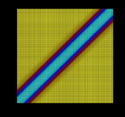
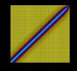
Figure 1: Top. Discrete Gaussian convolution operator $\bf V$. Bottom. 1-st order recursive filter operator $F_{1}$

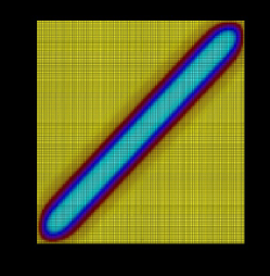
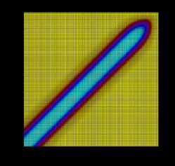
Figure 2: Top. 1-st order recursive filter operator $F^{(50)}_{1}$ with $50$ iterations. Bottom. 3-rd order recursive filter operator $F^{(1)}_{3}$

Figure 2 bottom shows that the operator $\bf F^{(1)}_{3}$ is closer then $\bf F^{(1)}_{1}$ and $\bf F^{(50)}_{1}$ to the discrete convolution $\bf V$. In particular, this recursive filter is able to reproduce $\bf V$ more accurately in the bottom left corner, but unfortunately it does not give good results on top right corner. In Table 2, for random distributions with homogeneous condition ($\sigma_{i}=\sigma$), we underline the edge effects by measuring the norms between the discrete convolution $\bf V$ and the RF filters. Although the $||\bf F_{n}^{(K)}-V||_{\infty}$ ideally goes to zero as $k$ goes to $+\infty$, this does not happen in practice as observed below.

Table 2: Distance metrics

$\sigma$	$||\bf F^{(1)}_{1}-V||_{\infty}$	$||\bf F^{(50)}_{1}-V||_{\infty}$	$||\bf F^{(1)}_{3}-V||_{\infty}$
5	0.2977	0.3800	0.5346
10	0.3895	0.4397	0.5890
25	0.4533	0.4758	0.6221
50	0.4686	0.4809	0.6125

In order to bring out these considerations, we show the application of $\bf V$, $\bf F^{(K)}_{1}$ and $\bf F^{(1)}_{3}$ to a periodic signal $\bf s^{0}$. We choose $m=252$ samples of the $\cos$ function in $[-2\pi,2\pi]$ and we perform simulations by using the 1-st RF with $1,5$ and $50$ iterations and 3-rd RF with one iteration. In Figure 3 it is shown the computed Gaussian convolution and the poor approximation of ${\bf V}s^{0}$ on the right side of the test interval, due to the edge effects. A nice result is that our $\bf F^{(1)}_{3}$ convolution operator gives better results on the left side of the domain.

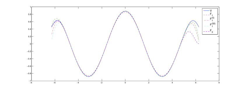
Figure 3: Discrete convolution $\bf V$ and Gaussian recursive filtering $\bf F^{(K)}_{1}$ with $1,5,50$ iterations and $\bf F^{(1)}_{3}$ applied to $n=252$ samples of the periodic function $s^{0}=\cos(x)$ in $[-2\pi,2\pi]$.

Finally, we give some considerations about the accuracy of the studied Gaussian RF schemes, when they are applied to the Dirac rectangular impulse

$s^{0}=(0,\ldots,0,1,0,\ldots).$

We choose a one-dimensional grid of $m=301$ points, a constant correlation radius $R=120,km$ , a constant grid space $\Delta x=6\,km$ and $\sigma=R/\Delta x=20$. In the numerical experiments to avoid the edge effects, we only consider $\bar{m}=221$ central values of $s^{K}$, i.e.

$\bar{s}^{K}=(s^{K}_{2\sigma},s^{K}_{2\sigma+1},\ldots,s^{K}_{m-2\sigma-1},s^{K}_{m-2\sigma})$.

Similarly, in Table 3 we measure the operator distances we use $\bf||\bar{F}^{(1)}_{1}-\bar{V}||_{\infty}$ and $\bf||\bar{F}^{(1)}_{3}-\bar{V}||_{\infty}$, where $\bar{V}$, $\bar{F}_{1}^{(1)}$ and $\bar{F}_{3}^{(1)}$ indicate the submatrices obtained, neglecting first and last $2\sigma-1$ rows and columns.

Table 3: Convergence history

K	$\bf||\bar{F}^{(K)}_{1}-\bar{V}||_{\infty}$	$\bf||\bar{F}^{(K)}_{3}-\bar{V}||_{\infty}$
1	0.211	0.0424
2	0.13	–
5	0.078	–
50	0.048	–
100	0.0429	–
500	0.0414	–

These case study shows that , neglecting the edge effects, the 3-rd RF filter is more accurate the the 1st-RF order with few iterations. This fact is evident by observing the results in Figure 4 and the operator norms in Table 3. Finally, we remark that the 1-st order RF has to use 100 iteration in order to obtain the same accuracy of the 3-rd order RF. This is a very interesting numerical feature of the third order filter.

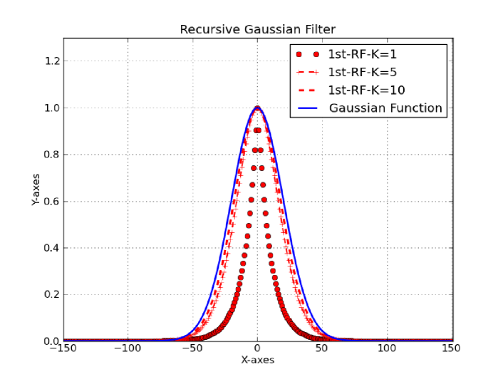
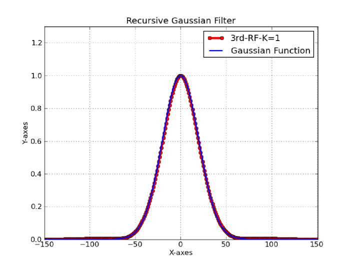
Figure 4: Top. The discrete Gaussian convolution ${\bf{V}}s^{0}$ (blue) and ${\bf{F}^{(K)}_{1}}s^{0}$ for $K=1,5,10$ (red). Bottom The discrete Gaussian convolution ${\bf{V}}s^{0}$ (blue) and ${\bf{F}^{(1)}_{3}}s^{0}$ (red).

V-B A case study: Ocean Var

The theoretical considerations of the previous sections are useful to understand the accuracy improvement in the real experiments on Ocean Var. The preconditioned CG is a numerical kernel intensively used in the model minimizations. Implementing a more accurate convolution operators gives benefits on the convergence of GC and on the overall data assimilation scheme [11] . Here we report experimental results of the 3rd-RF in a Global Ocean implementation of OceanVar that follows [21]. These results are extensively discussed in the report [11]. In real scenarios [4, 10] scientific libraries and an high performance computing environments are needed. The case study simulations were carried-out on an IBM cluster using 64 processors. The model resolution was about $1/4$ degree and the horizontal grid was tripolar, as described in [18]. This configuration of the model was used at CMCC for global ocean physical reanalyses applications (see [12]). The model has 50 vertical depth levels. The three-dimensional model grid consists of 736141000 grid-points. The comparison between the 1st-RF and 3rd-RF was carried out for a realistic case study, where all in-situ observations of temperature and salinity from Expendable bathythermographs (XBTs), Conductivity, Temperature, Depth (CTDs) Sensors, Argo floats and Tropical mooring arrays were assimilated. The observational profiles are collected, quality-checked and distributed by [3]. The global application of the recursive filter accounts for spatially varying and season-dependent correlation length-scales (CLSs). Correlation length-scale were calculated by applying the approximation given in [2] to a dataset of monthly anomalies with respect to the monthly climatology, with inter-annual trends removed.

The analysis increments from a 3DVAR applications that uses the 1st-RF with 1, 5 and 10 iterations and the 3rd-RF are shown in Figure 5 with a zoom in the same area of Western Pacific Area as in Figure 5, for the temperature at 100 m of depth. The Figure also displays the differences between the 3rd-RF and the 1st-RF with either 1 or 10 iterations. The patterns of the increments are closely similar, although increments for the case of 1st-RF (K=1) are generally sharper in the case of both short (e.g. off Japan) or long (e.g. off Indonesian region) CLSs. The panels of the differences reveal also that the differences between 3rd-RF and the 1st-RF (K=10) are very small, suggesting once again that the same accuracy of the 3rd-RF can be achieved only with a large number of iterations for the first order recursive filter. Finally, in [ARXIV] was also observed that the 3rd-RF compared to the 1st-RF (K=5) and the 1st-RF (K=10) reduces the wall clock time of the software respectively of about 27% and 48%.

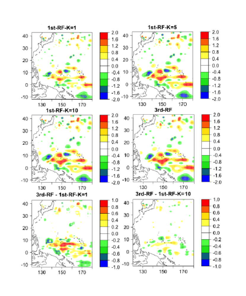
Figure 5: Analysis increments of temperature at 100 m of depth for the Western Pacific for different configurations of the recursive filter (first two rows of panels). Differences of 100 m temperature analysis increments between 3rd-RF and 1st-RF (K=1) and between 3rd-RF and 1st-RF (K=10) (bottom panels).

VI Conclusions

Recursive Filters (RFs) are a well known way to approximate the Gaussian convolution and are intensively applied in the meteorology, in the oceanography and in forecast models. In this paper, we deal with the oceanographic 3D-Var scheme OceanVar. The computational kernel of the OceanVar software is a linear system solved by means of the Conjugate Gradient (GC) method. The iteration matrix is related to an error covariance matrix, with a Gaussian correlation structure. In other words, at each iteration, a Gaussian convolution is required. Generally, this convolution is approximated by a first order RF. In this work, we introduced a 3rd-RF filter and we investigated about the main sources of error due to the use of 1st-RF and 3rd-RF operators. Moreover, we studied how these errors influence the CG algorithm and we showed that the third order operator is more accurate than the first order one. Finally, theoretical issues were confirmed by some numerical experiments and by the reported results in the case study of the OceanVar software.

References

- [1] M. Abramowitz, I. Stegun - Handbook of Mathematical Functions. Dover, New York, 1965.
- [2] M. Belo Pereira, L. Berre - The use of an ensemble approach to study the background-error covariances in a global NWP model. MOn. Wea. Rev. 134, pp. 2466-2489, 2006.
- [3] C. Cabanes, A. Grouazel, K. von Schuckmann, M. Hamon, V. Turpin, C. Coatanoan, F. Paris, S. Guinehut, C. Bppne, N. Ferry, C. de Boyer Montgut, T. Carval, G. Reverding, S. Puoliquen, P.Y. L. Traon - The CORA dataset: validation and diagnostics of in-situ ocean temperature and salinity measurements. Ocean Sci 9, pp. 1-18, 2013.
- [4] S. Cuomo, A. Galletti, G. Giunta and A. Starace-Surface reconstruction from scattered point via RBF interpolation on GPU , Federated Conference on Computer Science and Information Systems (FedCSIS), 2013, pp. 433-440.
- [5] G. Dahlquist and A. Bjorck - Numerical Methods. Prentice Hall, 573 pp. 1974.
- [6] J. Derber, A. Rosati - A global oceanic data assimilation system. Journal of Phys. Oceanogr. 19, pp. 1333-1347, 1989.
- [7] L. D’ Amore, R. Arcucci, L. Marcellino, A. Murli- HPC computation issues of the incremental 3D variational data assimilation scheme in OceanVarsoftware. Journal of Numerical Analysis, Industrial and Applied Mathematics, 7(3-4), pp 91-105, 2013.
- [8] R. Deriche - Separable recursive filtering for efficient multi-scale edge detection. Proc. Int. Workshop Machine Vision Machine Intelligence, Tokyo, Japan, pp 18-23, 1987
- [9] S. Dobricic, N. Pinardi - An oceanographic three-dimensional variational data assimilation scheme. Ocean Modeling 22, pp 89-105, 2008.
- [10] R. Farina, S. Cuomo, P. De Michele, F. Piccialli-A Smart GPU Implementation of an Elliptic Kernel for an Ocean Global Circulation Model, APPLIED MATHEMATICAL SCIENCES, 7 (61-64), 2013 pp.3007-3021.
- [11] R. Farina, S. Dobricic, S. Cuomo-Some numerical enhancements in a data assimilation scheme, AIP Conference Proceedings 1558, 2013, doi: 10.1063/1.4826017.
- [12] N. Ferry, B. Barnier, G. Garric, K. Haines, S. Masina, L. Parent, A. Storto, M. Valdivieso, S. Guinehut, S. Mulet - NEMO: the modeling engine of global ocean reanalysis. Mercator Ocean Quaterly Newsletter 46, pp 60-66, 2012.
- [13] S. Haben, A. Lawless, N. Nichols - Conditioning of the 3DVar data assimilation problem. University of Reading, Dept. of Mathematics, Math Report Series 3, 2009;
- [14] S. Haben, A. Lawless, N. Nicholos - Conditioning and preconditioning of the variational data assimilation problem. Computers and Fluids 46, pp 252-256, 2011.
- [15] L. Haglund - Adaptive multidimensional filtering. Linköping University, Sweden, 1992.
- [16] A.C. Lorenc - Iterative analysis using covariance functions and filters. Quartely Journal of the Royal Meteorological Society 1-118, pp 569-591, 1992.
- [17] A.C. Lorenc - Development of an operational variational assimilation scheme. Journal of the Meteorological Society of Japan 75, pp 339-346, 1997.
- [18] G. Madec, M. Imbard - A global ocean mesh to overcome the north pole singularity. Clim. Dynamic 12, pp 381-388, 1996.
- [19] R.J. Purser, W.-S. Wu, D.F. Parish, N.M. Roberts - Numerical aspects of the application of recursive filters to variational statistical analysis. Part II: spatially inhomogeneous and anisotropic covariances. Monthly Weather Review 131, pp 1524-1535, 2003.
- [20] C. Hayden, R. Purser - Recursive filter objective analysis of meteorological field: applications to NESDIS operational processing. Journal of Applied Meteorology 34, pp 3-15, 1995.
- [21] A. Storto, S. Dobricic, S. Masina, P. D. Pietro - Assimilating along-track altimetric observations through local hydrostatic adjustments in a global ocean reanalysis system. Mon. Wea. Rev. 139, pp 738-754, 2011.
- [22] L.V. Vliet, I. Young, P. Verbeek - Recursive Gaussian derivative filters. International Conference Recognition, pp 509-514, 1998.
- [23] L.J. van Vliet, P.W. Verbeek - Estimators for orientation and anisotropy in digitized images. Proc. ASCI’95, Heijen (Netherlands), pp 442-450, 1995.
- [24] A. T. Weaver, P. Courtier - Correlation modelling on the sphere using a generalized diffusion equation. Quarterly Journal of the Royal Meteorological Society 127, pp 1815-1846, 2001.
- [25] A. Witkin - Scale-space filtering. Proc. Internat. Joint Conf. on Artificial Intelligence, Karlsruhe, germany, pp 1019-1021, 1983.
- [26] I.T. Young, L.J. van Vliet - Recursive implementation of the Gaussian filter. Signal Processing 44, pp 139-151, 1995.