Convective overstability in accretion disks
3D linear analysis and nonlinear saturation

Abstract

Recently, Klahr & Hubbard (2014) claimed that a hydrodynamical linear overstability exists in protoplanetary disks, powered by buoyancy in the presence of thermal relaxation. We analyse this claim, confirming it through rigorous compressible linear analysis. We model the system numerically, reproducing the linear growth rate for all cases studied. We also study the saturated properties of the overstability in the shearing box, finding that the saturated state produces finite amplitude fluctuations strong enough to trigger the subcritical baroclinic instability. Saturation leads to a fast burst of enstrophy in the box, and a large-scale vortex develops in the course of the next $\approx$100 orbits. The amount of angular momentum transport achieved is of the order of $\alpha\approx 10^{-3}$, as in compressible SBI models. For the first time, a self-sustained 3D vortex is produced from linear amplitude perturbation of a quiescent base state.

1. Introduction

Accretion in disks is generally thought to occur by the action of turbulence, for which the magnetorotational instability (MRI, Balbus & Hawley, 1991) is the most likely culprit. However, protoplanetary disks are cold; the ionization level required to couple the gas to the ambient field is not always met (Blaes & Balbus, 1994), leading to zones that are “dead” to the MRI (Gammie, 1996; Turner & Drake, 2009). So, the quest for hydrodynamical sources of turbulence continues, if only to provide accretion through this dead zone.

One such possible sources of hydrodynamical turbulence is the subcritical baroclinic instability (SBI, Klahr & Bodenheimer, 2003; Klahr, 2004; Petersen et al., 2007a, b; Lesur & Papaloizou, 2010; Lyra & Klahr, 2011; Raettig et al., 2013), a process shown to sustain large-scale vortices in the presence of a radial entropy gradient and thermal relaxation or diffusion. Two-dimensional linear stability analysis and numerical simulations do not find instability if only seeded with linear noise (Johnson & Gammie, 2005), though it was shown that finite amplitude perturbations would trigger it, concluding that the instability is nonlinear in nature (Lesur & Papaloizou, 2010). Characterization of the instability through nonlinear numerical simulations shows that maximum amplification is found for thermal times in the range of 1–10 times the dynamical timescale (Lesur & Papaloizou, 2010; Lyra & Klahr, 2011; Raettig et al., 2013). Although no criterion for a critical Reynolds number was derived, Raettig et al. (2013) show that as resolution is increased, ever smaller perturbations are necessary, as expected if the process is physical. Compressible simulations (Lesur & Papaloizou, 2010; Lyra & Klahr, 2011) show that the spiral density waves excited by the vortices (Heinemann & Papaloizou, 2009a, b, 2012) transport angular momentum at the level of $\alpha\approx 10^{-3}$, where $\alpha$ is the Shakura-Sunyaev parameter Shakura & Sunyaev (1973). If this process indeed occur in disks, it would provide not only accretion but also a fast route for planet formation in the dead zone, since vortices speed up the process enormously, by concentrating particles in their centers (Barge & Sommeria, 1995; Klahr & Bodenheimer, 2006; Lyra et al., 2008b, 2009).

The appeal of the SBI, however, is severely hindered by its nonlinear nature. Without the guide of analytics, nonlinear processes are difficult to characterize, and the accuracy of the numerics have to be well-established beyond reasonable doubts. Recently, Klahr & Hubbard (2014, hereafter KH14) have claimed that, when considering the same equations that lead to SBI in 2D, linear growth exists if vertical wavelengths are considered. The unstable mode is a slowly growing epicyclic oscillation, which led the authors to name the process “convective overstability”. Growth is powered by buoyancy and thermal relaxation in the same regime as the SBI, of cooling time of the order of the dynamical time. We analyze this claim of linearity in more detail in this paper. Independent verification is desirable since unorthodox assumptions were made in the linear analysis of KH14. In particular, the authors assumed that the timescale for pressure equilibration is fast, and thus set the pressure perturbation to zero in the linear analysis. Because of this strong assumption, skepticism about the validity of the work naturally remains until a rigorous derivation of the dispersion relation is provided, unambiguously demonstrating that the eigenvector of the growing root has no appreciable pressure term. In this work, we provide such derivation.

Another point raised by KH14 is the connection between this overstability and the SBI, if any. A priori, the two processes have little to do with each other. However, as the regimes of cooling time for both are similar, if the convective overstability exists, it may generate the finite amplitude perturbations that trigger the SBI. In this scenario, the (nonlinear) SBI would simply be the saturated state of the (linear) convective overstability. Since the difficulty on finding a source of finite amplitude perturbation in dead zones in the required range of cooling times had made the SBI look less attractive as a relevant disk process, a linear process that can spawn the SBI from arbitrarily low-level noise would be particularly interesting. Conversely, there is the possibility, of course, that the saturated state of the convective overstability may still be of too low amplitude to trigger the SBI. We investigate these possibilities in the present study.

This paper is structured as follows. In Sect 2 we perform a linear analysis calculating the full compressible dispersion relation. In Sect 3 we take the anelastic limit to derive the instability criterion, finding the roots, the most unstable mode, and associated eigenvector. In Sect 4 we perform numerical simulations in the shearing box to characterize the linear growth phase and nonlinear saturation in 2D and 3D. We conclude in Sect 5.

Table 1Symbols used in this work

Symbol	Definition	Description
$r$		cylindrical radial coordinate
$\phi$		azimuth
$r_{0}$		reference radius
$x$	$=r-r_{0}$	Cartesian radial coordinate
$y$	$=r\phi$	Cartesian azimuthal coordinate
$z$		vertical coordinate
$k_{r},k_{x}$		radial wavenumber
$m$		azimuthal wavenumber
$k_{z}$		vertical wavenumber
$k$	$=\sqrt{k_{r}^{2}+k_{z}^{2}}$
$\mu$	$=k_{z}/k$
$t$		time
$\rho$		density
${\boldsymbol{u}}$		velocity
$T$		temperature
$\gamma$		adiabatic index
$c_{p}$		specific heat at constant pressure
$c_{v}$	$=c_{p}/\gamma$	specific heat at constant volume
$p$	$=c_{v}(\gamma-1)\rho T$	pressure
$\tau$		thermal time
$\varsigma$	$=\nicefrac{{1}}{{\gamma\tau}}$
$\varOmega$		Keplerian angular frequency
$q$	$=-d\ln\varOmega/d\ln r$	shear parameter
$\kappa$	$=\sqrt{2(2-q)}\ \varOmega$	epicyclic frequency
$\alpha$	$=d\ln\rho/d\ln r$	density gradient
$\beta$	$=d\ln T/d\ln r$	temperature gradient
$\xi$	$=\alpha+\beta$	pressure gradient
$\omega$		complex eigenfrequency
$\bar{\omega}$	$=\omega-m\varOmega$
$s$	$={\rm Re}(\bar{\omega})$	oscillation frequency
$\sigma$	$={\rm Im}(\bar{\omega})$	growth rate
$c$	$=\left[T\ c_{p}(\gamma-1)\right]^{1/2}$	sound speed
$A$	$=c\ \partial_{r}\ln\rho$
$B$	$=\gamma^{-1}c\ \partial_{r}\ln p$
$N$	$=\sqrt{AB-B^{2}}$	Brunt-Väisälä frequency
$a$	$=A/c$
$b$	$=B/c$
$H$	$=c/\varOmega$	disk scale height
$h$	$=H/r$	disk aspect ratio
$\varSigma$	$\propto\rho H$	surface density
$\psi$	$=d\ln\varSigma/d\ln r$	surface density gradient

2. Linear dispersion relation

Let us consider the compressible Euler equations with thermal relaxation.

$$\frac{\partial{\rho}}{\partial{t}}+\left({\boldsymbol{u}}\cdot{\boldsymbol{\nabla}}\right)\rho = -\rho{\boldsymbol{\nabla}}\cdot{\boldsymbol{u}},$$ (1)

$$\frac{\partial{{\boldsymbol{u}}}}{\partial{t}}+\left({\boldsymbol{u}}\cdot{\boldsymbol{\nabla}}\right){\boldsymbol{u}} = -\frac{1}{\rho}{\boldsymbol{\nabla}}{p}+{\boldsymbol{g}},$$ (2)

$$\frac{\partial{p}}{\partial{t}}+\left({\boldsymbol{u}}\cdot{\boldsymbol{\nabla}}\right)p = -\gamma p{\boldsymbol{\nabla}}\cdot{\boldsymbol{u}}-\frac{p}{T}\frac{(T-T_{0})}{\tau},$$ (3)

where $\rho$ is the density, ${\boldsymbol{u}}$ is the velocity, $p$ is the pressure, $\gamma$ is the adiabatic index, $T$ is the temperature, $T_{0}$ is a reference temperature, and $\tau$ is the thermal time. We consider the cylindrical approximation, meaning that we omit the vertical component of the stellar gravity, as well as vertical stratification. In this approximation, the gravity is ${\boldsymbol{g}}=-\varOmega^{2}{\boldsymbol{r}}$, with $\varOmega$ the Keplerian angular frequency and ${\boldsymbol{r}}$ the cylindrical radial coordinate. A list of the mathematical symbols used in this work, together with their definitions, is provided in Table 1.

We linearize Eqs. (1)–(3) into base state and perturbation (the latter denoted by primes), as $u_{r}=u_{r}^{\prime}$, $u_{\phi}=u_{\phi}^{\prime}+\varOmega r$, $u_{z}=u_{z}^{\prime}$, $p=p_{0}+p^{\prime}$, and $\rho=\rho_{0}+\rho^{\prime}$. Assuming the cylindrical approximation ($\partial_{z}$ =0 for the base state), Eqs. (1)–(3) become

$$\partial_{\hat{t}}\rho^{\prime}+u_{r}^{\prime}\partial_{r}\rho_{0}+\rho_{0}{\boldsymbol{\nabla}}\cdot{{\boldsymbol{u}}^{\prime}} = 0,$$ (4)

$$\partial_{\hat{t}}u_{r}^{\prime}-2\varOmega u_{\phi}^{\prime}+\frac{1}{\rho_{0}}\partial_{r}p^{\prime}-\frac{\rho^{\prime}}{\rho_{0}^{2}}\partial_{r}p_{0} = 0,$$ (5)

$$\partial_{\hat{t}}u_{\phi}^{\prime}+\varOmega(2-q)u_{r}^{\prime}+\frac{1}{\rho_{0}}\partial_{\hat{\phi}}p^{\prime} = 0,$$ (6)

$$\partial_{\hat{t}}u_{z}^{\prime}+\frac{1}{\rho_{0}}\partial_{z}p^{\prime} = 0,$$ (7)

$$\partial_{\hat{t}}p^{\prime}+u_{r}^{\prime}\partial_{r}p_{0}+\gamma p_{0}{\boldsymbol{\nabla}}\cdot{{\boldsymbol{u}}^{\prime}}+\frac{p^{\prime}}{\tau}-\frac{p_{0}\rho^{\prime}}{\rho_{0}\tau} = 0.$$ (8)

Figure 1.— The sign of the square of the Brunt-Väisälä frequency defines the stability criterion, here shown as a function of the density and temperature power-law indices. The plot shows the lines for two values of $\gamma$. Above (below) the respective line the system is stable (unstable).

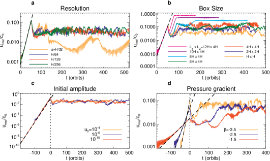
Figure 2.— Convergence study of the saturated state of the overstability. a, the box size ($H{\times}H$), initial amplitude ($u_{\rm rms}/c=10^{-3}$) and pressure gradient ($\xi=-3.5$) were kept fixed, while the resolution was changed. Saturation occurs at 64 points per scale height. b, The resolution is fixed at $\Delta=H/64$, and the box size changed. There is no convergence with box size (see fig 3 and discussion in the text). c, resolution $\Delta=H/64$, box size $H{\times}H$, and varying initial amplitude. d., varying the pressure gradient, resolution $\Delta=H/64$, box size 2H. Amplitude converges in both latter cases. The linear growth rate (black dashed line) is very well reproduced in all cases.

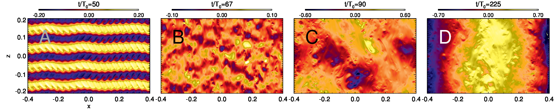
Figure 3.— Spectral description of the $8H{\times}4H$ simulation (cyan line in fig 2, upper right). The rms velocity is shown in the upper left panel, with four representative points marked, and the velocity shown, in the xz plane, in each of these points (lower panels). The points are: $A$, onset of saturation; $B$, the local minimum; $C$, second saturated state; $D$, state after the last bifurcation. The spectral power in the first 5 large-scale modes in $x$ and $z$ is shown in the upper middle and right panels, respectively. Point $A$ corresponds to Kelvin-Helmholtz instability breaking up the original $k_{z}/k_{z0}=4$ channel mode, as nonzero $k_{x}$ and $k_{z}$ modes are excited. The local minimum $B$ corresponds to the point when power is equally distributed among the non-zero $k_{z}$ modes. The saturated state $C$ corresponds to dominance of the $k_{z}=1$ mode, with a mixed $k_{x}=1$ mode (both clear in the lower “C” panel). The last bifurcation corresponds to the $k_{z}=0$ mode taking over, and a large scale $k_{x}=1$ dominating the box.

In the above equations, $\partial_{\hat{t}}=\partial_{t}+\varOmega\partial_{\phi}$, $\partial_{\hat{\phi}}=r^{-1}\ \partial_{\phi}$, ${\boldsymbol{\nabla}}\cdot{{\boldsymbol{u}}^{\prime}}=\partial_{r}u_{r}^{\prime}+u_{r}^{\prime}/r+\partial_{\hat{\phi}}u_{\phi}^{\prime}+\partial_{z}u_{z}^{\prime}$, and the thermal relaxation term was linearized

$$\frac{\delta T}{T}=\frac{\delta p}{p}-\frac{\delta\rho}{\rho},$$

as per the equation of state, $p=c_{v}(\gamma-1)\rho T$. Next we use the short-wave approximation, $m\ll k_{r}r,k_{z}z$, and expand the perturbations in Fourier modes, $\exp(-i\omega t+ik_{r}r+im\phi+ik_{z}z)$. Eqs. (4)–(8) then become

$$-i\bar{\omega}\rho^{\prime}+u_{r}^{\prime}\partial_{r}\rho_{0}+\rho_{0}ik_{r}u_{r}^{\prime}+\rho_{0}ik_{z}u_{z}^{\prime} = 0$$ (9)

$$-i\bar{\omega}u_{r}^{\prime}-2\varOmega u_{\phi}^{\prime}+ik_{r}\rho_{0}^{-1}p^{\prime}-\frac{\rho^{\prime}}{\rho_{0}^{2}}\partial_{r}p_{0} = 0$$ (10)

$$-i\bar{\omega}u_{\phi}^{\prime}+\varOmega(2-q)u_{r}^{\prime} = 0$$ (11)

$$-i\bar{\omega}u_{z}^{\prime}+ik_{z}\rho_{0}^{-1}p^{\prime} = 0$$ (12)

$$-i\bar{\omega}p^{\prime}+u_{r}^{\prime}\partial_{r}p_{0}+\rho_{0}c^{2}ik_{r}u_{r}^{\prime}+\rho_{0}c^{2}ik_{z}u_{z}^{\prime}$$

$$+\frac{p^{\prime}}{\tau}-\frac{c^{2}\rho^{\prime}}{\gamma\tau} = 0$$ (13)

where $\bar{\omega}=\omega-m\varOmega$, and we have also substituted $p_{0}=\rho_{0}c^{2}/\gamma$. The system is $\boldsymbol{\mathrm{M}}\cdot{\boldsymbol{\upsilon}}=0$, where ${\boldsymbol{\upsilon}}=[\rho^{\prime},u_{r}^{\prime},u_{\phi}^{\prime},u_{z}^{\prime},p^{\prime}]^{T}$, and the coefficient matrix is

$$\boldsymbol{\mathrm{M}}=\left[\begin{array}[]{ccccc}-i\bar{\omega}&\rho_{0}(ik_{r}+\nicefrac{{A}}{{c}})&0&\rho_{0}ik_{z}&0\\ -\nicefrac{{Bc}}{{\rho_{0}}}&-i\bar{\omega}&-2\varOmega&0&\nicefrac{{ik_{r}}}{{\rho_{0}}}\\ 0&\varOmega(2-q)&-i\bar{\omega}&0&0\\ 0&0&0&-i\bar{\omega}&\nicefrac{{ik_{z}}}{{\rho_{0}}}\\ -\nicefrac{{c^{2}}}{{\gamma\tau}}&\rho_{0}c^{2}(ik_{r}+\nicefrac{{B}}{{c}})&0&\rho_{0}c^{2}ik_{z}&-i\bar{\omega}+\nicefrac{{1}}{{\tau}}\\ \end{array}\right].$$ (14)

We have substituted

$$A = {\color[rgb]{1,1,1}\gamma^{-1}}c\ \partial_{r}\ln\rho,$$ (15)

$$B = \gamma^{-1}c\ \partial_{r}\ln p,$$ (16)

so both $A$ and $B$ have dimension of frequency. In particular, $AB=1/\rho^{2}\partial_{r}\rho\partial_{r}p$, and $B^{2}=(\gamma\rho p)^{-1}(\partial_{r}p)^{2}$, so $N^{2}=AB-B^{2}$ is the square of the Brunt-Väisälä frequency. The full dispersion relation ${\rm det}\boldsymbol{\mathrm{M}}=0$ is

$$\bar{\omega}^{5}+\bar{\omega}^{4}\ i\tau^{-1}-\bar{\omega}^{3}\ (AB+c^{2}k^{2}+\kappa^{2})$$ (17)

$$+ \bar{\omega}^{2}\ \tau^{-1}\left[k_{r}c(B-A\gamma^{-1})-i(AB+c^{2}k^{2}\gamma^{-1}+\kappa^{2})\right]$$

$$+ \bar{\omega}\ c^{2}k_{z}^{2}(\kappa^{2}+N^{2})+\frac{ic^{2}\kappa^{2}k_{z}^{2}}{\gamma\tau}=0,$$

where $\kappa^{2}=2(2-q)\varOmega^{2}$ is the square of the epicyclic frequency. We consider now some limits of Eq. (17).

3. Anelastic limit

In the anelastic limit, $c=\infty$, Eq. (17) reduces to

$$\bar{\omega}^{3}k^{2}-\bar{\omega}^{2}\ \tau^{-1}\left[k_{r}(b-a/\gamma)-ik^{2}\gamma^{-1}\right]$$

$$-\bar{\omega}\ k_{z}^{2}(\kappa^{2}+N^{2})-\frac{i\kappa^{2}k_{z}^{2}}{\gamma\tau} = 0,$$ (18)

where $b=B/c=\gamma^{-1}\partial_{r}\ln p$ and $a=A/c=\partial_{r}\ln\rho$. These terms are proportional to $1/r$, so they are small and can be dropped. The dispersion relation is thus

$$\bar{\omega}^{3}+i\varsigma\bar{\omega}^{2}-\bar{\omega}\mu^{2}(\kappa^{2}+N^{2})-i\varsigma\kappa^{2}\mu^{2}=0,$$ (19)

where we have also substituted $\varsigma=1/\gamma\tau$ and $\mu^{2}=k_{z}^{2}/k^{2}$.

3.1. Adiabatic

For adiabatic flow, $\tau=\infty$, Eq. (19) reduces to

$$\bar{\omega}^{2}=\mu^{2}\left(\kappa^{2}+N^{2}\right)$$ (20)

For $k_{r}=0$ (in-plane incompressible motion), we retrieve $\bar{\omega}^{2}=\kappa^{2}+N^{2}$, the Solberg-Hoiland criterion.

3.2. Finite $\tau$, $k_{r}=0$

For pure in-plane incompressible motions ($k_{r}=0$), Eq. (19) reduces to

$$\bar{\omega}^{3}+\bar{\omega}^{2}i\varsigma-\bar{\omega}(\kappa^{2}+N^{2})-i\varsigma\kappa^{2}=0,$$ (21)

which is the same as derived by KH14 (their eq. 18), using other assumptions.

3.3. Finite $\tau$, $k_{r}\neq 0$

Substituting $\bar{\omega}=s+i\sigma$, growing solutions correspond to real positive $\sigma$. The dispersion relation, real and imaginary, that need to vanish independently, are:

$$s^{2}=\mu^{2}(N^{2}+\kappa^{2})+3\sigma^{2}+2\sigma\varsigma;$$ (22)

$$\sigma^{3}+\sigma^{2}\varsigma-\sigma[3s^{2}-\mu^{2}(N^{2}+\kappa^{2})]-\varsigma(s^{2}-\mu^{2}\kappa^{2})=0.$$ (23)

Substituting Eq. (22) into Eq. (23), we get

$$2\sigma(2\sigma+\varsigma)^{2}+2\sigma\mu^{2}(\kappa^{2}+N^{2})+\mu^{2}\varsigma N^{2}=0.$$ (24)

As we expect the growth to be small (to be checked a posteriori), we take the limit $\sigma\ll\varsigma$, leading to

$$\sigma=-\frac{1}{2}\left[\frac{\mu^{2}\varsigma N^{2}}{\varsigma^{2}+\mu^{2}(\kappa^{2}+N^{2})}\right].$$ (25)

This function has no extrema for finite $\mu$. For $\varsigma$, however, there is a maximum at $\varsigma^{2}|_{{}_{d_{t}\sigma=0}}=\varsigma_{\rm max}^{2}=\mu^{2}(\kappa^{2}+N^{2})$, that is, maximum growth occurs for

$$\tau_{\rm max}=\frac{1}{\gamma}\left|\frac{k}{k_{z}}\right|\frac{1}{\sqrt{\kappa^{2}+N^{2}}}$$ (26)

for which the growth rate is $\sigma_{\max}=-\mu^{2}N^{2}/(4\varsigma_{\rm max})$, i.e.

$$\sigma_{\rm max}=-\frac{1}{4}\left|\frac{k_{z}}{k}\right|\frac{N^{2}}{\sqrt{\kappa^{2}+N^{2}}}$$ (27)

3.3.1 Keplerian disks

Recalling the definition of the Brunt-Väisälä frequency

$$N^{2}\equiv\frac{1}{\rho}\frac{dp}{dr}\left(\frac{1}{\rho}\frac{d\rho}{dr}-\frac{1}{\gamma p}\frac{dp}{dr}\right),$$ (28)

we can write it in terms of the power-law indices of the density and temperature gradients, $\alpha=\partial\ln\rho/\partial\ln r$, $\beta=\partial\ln T/\partial\ln r$, and $\xi=\alpha+\beta=\partial\ln p/\partial\ln r$, resulting in

$$N^{2}=\frac{\varOmega^{2}h^{2}}{\gamma}\left(\alpha\xi-\frac{1}{\gamma}\xi^{2}\right),$$ (29)

where $h=H/r$ is the aspect ratio and $H=c/\varOmega$ is the scale height. So, for Keplerian disks, $\kappa=\varOmega$ and $|N^{2}|\sim\varOmega^{2}\mathcal{O}(h^{2})$. It results from this that $\tau_{\rm max}$ is of order $1/\varOmega$, while the associated growth rate is of order $\sigma_{\rm max}=\varOmega\mathcal{O}(h^{2})$, validating the assumption that $\sigma\ll\varsigma$.

Notice that for $k_{r}\gg k_{z}$, that is, $\mu^{2}\rightarrow 0$, the dispersion relation (Eq. 24) becomes

$$\sigma(2\sigma+\varsigma)^{2}=0,$$ (30)

for which the roots are $\sigma=0$, and $\sigma=-\varsigma/2$, that is, no growth, and damped perturbations. For channel modes ($k_{r}=0$) in Keplerian disks ($\kappa=\varOmega\gg|N|$), we find

$$\tau_{\rm max} = {\color[rgb]{1,1,1}+}\frac{1}{\gamma\varOmega};$$ (31)

$$\sigma_{\rm max} = -\frac{N^{2}}{4\varOmega}.$$ (32)

We plot in 1 the unstable range as a function of the density and temperature power law indices.

3.4. The unstable mode

To understand the most unstable mode, we check the eigenvector ${\boldsymbol{\upsilon}}_{\rm max}$ corresponding to this root, for which the eigenvalue is

$$\lambda=i\omega_{\rm max}=i\varOmega-\sigma_{\rm max},$$ (33)

and the system is $\boldsymbol{\mathrm{R}}\cdot{\boldsymbol{\upsilon}}_{\rm max}=\lambda{\boldsymbol{\upsilon}}_{\rm max}$, where

$$\boldsymbol{\mathrm{R}}=\left[\begin{array}[]{ccccc}0&\rho_{0}\nicefrac{{A}}{{c}}&0&\rho_{0}ik_{z}&0\\ -\nicefrac{{Bc}}{{\rho_{0}}}&0&-2\varOmega&0&0\\ 0&\varOmega/2&0&0&0\\ 0&0&0&0&\nicefrac{{ik_{z}}}{{\rho_{0}}}\\ -c^{2}\varOmega&\rho_{0}Bc&0&\rho_{0}c^{2}ik_{z}&\gamma\varOmega\\ \end{array}\right].$$ (34)

The 4th line is $ik_{z}/\rho_{0}u_{z}^{\prime}=i\varOmega u_{z}^{\prime}-\sigma_{\rm max}u_{z}^{\prime}$, which is only satisfied for the trivial solution $u_{z}^{\prime}$=0. The reduced system becomes

$$\rho^{\prime} = \lambda^{-1}\rho_{0}a\ u_{r}^{\prime};$$ (35)

$$u_{\phi}^{\prime} = \lambda^{-1}\varOmega/2\ u_{r}^{\prime};$$ (36)

$$p^{\prime} = (\lambda-\gamma\varOmega)^{-1}\left(\rho_{0}cBu_{r}^{\prime}-c^{2}\varOmega\rho^{\prime}\right).$$ (37)

The solution is

$$\ln\rho^{\prime} = -\frac{\sigma+i\varOmega}{\varOmega}au_{r}^{\prime};$$ (38)

$$u_{\phi}^{\prime} = -\frac{\sigma+i\varOmega}{2\varOmega}u_{r}^{\prime};$$ (39)

$$\ln p^{\prime} = -\gamma\left(\frac{\sigma}{\varOmega}a+b\right)\left[\frac{\sigma+\varOmega\gamma+i\varOmega}{(\sigma+\gamma\varOmega)^{2}+\varOmega^{2}}\right]u_{r}^{\prime}.$$ (40)

Since $\sigma\ll\varOmega$, the pressure perturbation is

$$\ln p^{\prime}=-\frac{\gamma(\gamma+i)}{\varOmega(\gamma+1)}bu_{r}^{\prime}.$$ (41)

And, because $a$ and $b$ are or order $\nicefrac{{1}}{{r}}$, $\ln\rho^{\prime}$ and $\ln p^{\prime}$ are vanishingly small. That the pressure variation does not play a major role in the instability justifies (now a posteriori) the $p^{\prime}=0$ approximation of KH14. The eigenvector is simply

$${\boldsymbol{\upsilon}}_{\rm max}=\left[0,1,-\frac{1}{2}\left(\frac{\sigma}{\varOmega}+i\right),0,0\right]^{T},$$ (42)

i.e., an overstable epicycle.

Figure 4.— Nonlinear evolution of the buoyant overstability in three dimensions. With the linear overstability raising the amplitude of the initial fluctuations to nonlinear levels, the saturated state is expected to be similar to that of the SBI. In the lower left panels we show the averaged vertical vorticity; the lower right shows the vorticity in the 3D flow. Indeed, we see that large-scale self-sustained anticyclonic vortices develop in the saturated state. The upper left panel shows the radial velocity rms and vertical enstrophy (red and black line, respectively.) The upper right panel shows the level of Reynolds stress, saturating at $\alpha\approx 10^{-3}$.

4. Numerical simulations

We now turn to numerical simulations to check the evolution of the instability. We use the shearing box model of Lyra & Klahr (2011), that includes the linearized pressure gradient. We do so in order to benefit from shear-periodic boundaries, in contrast to the simulations in the appendix of KH14, that are affected by radial boundaries. The reader is referred to Lyra & Klahr (2011) for the equations of motion, properties and caveats of the approximation. In particular, the density gradient is zero, and we drop the $x$-dependent term in the pdV work to keep shear-periodicity (see appendix A of Lyra & Klahr (2011).

We solve the evolution equations with the Pencil Code (Brandenburg & Dobler, 2002) which integrates the PDEs with sixth order spatial derivatives, and a third order Runge-Kutta time integrator. Sixth-order hyper-dissipation terms are added to the evolution equations, to provide extra dissipation near the grid scale, explained in Lyra et al. (2008a). They are needed because the high-order scheme of the Pencil Code has little overall numerical dissipation (McNally et al., 2012).

We run a suite of 2D axisymmetric models ($x$ and $z$) to understand the linear evolution and saturation properties of the instability. The sound speed is $c$=0.1, and the adiabatic index is $\gamma=1.4$. The cooling time is $\tau_{\rm max}=\nicefrac{{1}}{{\gamma\varOmega}}$. Our units are $\varOmega=c_{p}=\rho_{0}=1$.

We initialize the simulations with the eigenvector corresponding to the epicycle oscillation, $u_{y}=-iu_{x}/2$. Because for $k_{x}=0$ the growth rate does not depend on $k_{z}$, we arbitrarily choose $\lambda_{z}=H$ for the channel mode. The initial condition therefore is

$$u_{x} = u_{0}\sin\left(\frac{2\pi}{H}z\right);$$ (43)

$$u_{y} = \frac{u_{0}}{2}\cos\left(\frac{2\pi}{H}z\right).$$ (44)

The fiducial model has resolution $\Delta{x}=\Delta{z}=H/64$, box size $L_{x}\times L_{z}=2H\times 2H$, temperature gradient $\beta=-3.5$, and initial amplitude $u_{0}/c=10^{-3}$. We vary these quantities to check convergence at saturation. The evolution of the 2D axisymmetric box seeded with the channel mode is shown in the panels of 2. The linear phase matches the analytical prediction (dashed black line) for all models ran.

Figure 2a shows the dependency on resolution. Convergence is achieved for 64 grid points per scale height. There is also convergence for initial amplitude of perturbation, as seen in 2c. The linear phase is identical in the three cases examined ($u_{0}=10^{-4},10^{-6}$, and $10^{-10}$). In this figure we set $t=0$ as the time that saturation is achieved, to better compare the nonlinear evolution. In 2d we check how the instability depends on the pressure gradient. Again, the linear phase is reproduced for the different values of the Brunt-Väisälä frequency, and the amplitudes at saturation are similar, within a factor 2–3. Difference in seen when we test the dependency on box size (2b). The amplitude seemed to saturate at $4H{\times}4H$ (red line), since the model with $L_{x}=6H$ (green line) shows a similar amplitude. However, the model with $L_{x}=8H$ (cyan line) shows a bifurcation at $\approx$150 orbits. Models with larger radial range ($L_{x}=10$ and $L_{x}=12$, purple and magenta lines, respectively) show no convergence, even as the velocity dispersion increasingly approaches the sound speed.

Interesting features are seen in this simulation, that help understand the behavior of the system. We plot in 3 the time evolution of the power in the first 5 large scale modes, in both $x$ (upper middle panel) and $z$ (upper left panel). The upper left panel shows the rms of the radial velocity. Four special/representative instants are labeled, and the $u_{x}$ field for these respective instants are shown in the lower panels.

The first instant, $A$, corresponds to the first “saturation” seen at 50 orbits. The power spectrum shows that the clean initial channel mode ($k_{z}/k_{z0}$=4, $k_{x}/k_{x0}$=0) persisted until this time, after which it saturates, exciting $k_{x}\neq 0$ modes and other $k_{z}$ modes. Instant $B$, at 67 orbits, corresponds to the local minimum in rms velocity. The power spectrum shows that this happens when the $k_{z}/k_{z0}$=1 mode becomes dominant. Subsequently, this mode keeps growing, at the same rate as the initial $k_{z}/k_{z0}$=4 mode. This is because the growth rate is independent of $k_{z}$ for $k_{x}=0$, which at that time has similar power as the higher $k_{x}$ modes. From time $t$=90 (instant $C$) to 160 orbits the system settles into a steady state, with a dominant $k_{z}/k_{z0}$=1 mode, and mixed $k_{x}/k_{x0}$=0 and $k_{x}/k_{x0}$=1. Another bifurcation happens when the $k_{z}=0$ mode overtakes the $k_{z}/k_{z0}$=1 mode. Simultaneously, it prompts $k_{x}/k_{x0}$=1 to dominate over $k_{x}=0$. The final state (labeled $D$) is thus vertically symmetric, with a box-wide radial wavelength.

This explains why we do not find convergence while increasing box vertical range from $L_{z}$=$H$ to $2H$ to $4H$. In these boxes, because we kept the seed mode at $k_{z}=2\pi/H$, we initialized the instability with the $k_{z}/k_{z0}$=1, 2, and 4 mode, respectively. In the last two simulations, the $k_{z}/k_{z0}$=1 mode was growing, with less power, but eventually catching up as the seed mode saturates. Convergence with radial box size is never achieved in the 2D runs because the $k_{x}/k_{x0}=1$ mode comes to dominate, no matter how wide we make the box. The simulations with radial box size $L_{x}=10H$ and $L_{x}=12H$ show the same pattern, albeit with no intermediate phase of dominance of a $k_{z}/k_{z0}$=1 mode.

4.1. 3D instability: growth of large-scale vortices

Next we turn to the 3D evolution of the instability. We set a box of size $4H\times 16H\times 2H$, with resolution $256\times 256\times 128$ in $x$, $y$, and $z$, respectively. The cells thus have aspect ratio $1\times 4\times 1$ (we have checked in Lyra & Klahr 2011 that unit aspect ratio in $x$ and $y$ gave the same results for the twodimensional SBI).

With the azimuthal direction present, vertical vorticity (in-plane circulation) can evolve unabridged. We show in 4 (left panel) the evolution of the rms velocity (red line) and enstrophy (black line). When the initial $k_{z}$ mode saturates (at 50 orbits, as in the 2D meridional models of fig 3), a sharp rise in enstrophy occurs. The situation is now very similar to the SBI, with high-amplitude perturbations ($u_{\rm rms}\approx 0.1c_{s}$), thermal relaxation, and an entropy gradient. The nonlinear saturation state of this buoyant overstability should thus proceed very similarly to the evolution of the SBI. Indeed, as the lower panels of 4 show, the saturated state develops into a large scale vortex. The amount of angular momentum transport (4, upper right) is at the $\alpha\approx 10^{-3}$ level, again, the typical level of the SBI. It seems conclusive that the saturated state of the buoyant overstability is the SBI.

5. Conclusions

We conclude that indeed there is a linear overstability in the region of the parameter space of negative $N^{2}$, finite cooling time $\tau$, and non-zero $k_{z}$ perturbation. The approximation $\delta p=0$ done by KH14 is justified as $\delta p=0$ (and $\delta\rho$) in the eigenvector of the most unstable modes is vanishingly small in comparison to the velocity amplitude (Eq. 42).

Modeling the system numerically, we reproduce the linear growth rate in all cases. In the twodimensional meridional simulations, we find convergence in the saturated state with resolution, but not with box size, since a large-scale $k_{x}/k_{x0}=1$ radial mode dominates the box. However, in three dimensions this mode does not show up, as it gets sheared away.

We also show that the SBI is indeed the saturated state of the overstability. Saturation leads to a fast burst of enstrophy in the box, and a large-scale vortex develops in the course of the next $\approx$100 orbits after the convective overstability has built the finite amplitude perturbations. The amount of angular momentum transport achieved is of the order of $\alpha\approx 10^{-3}$, as in compressible SBI models.

It remains to be shown if these processes (both SBI and convective overstability) operate in global models, i.e., how they respond to boundary conditions and curvature terms. The relation between this overstability and the Goldreich-Schubert-Fricke instability (Goldreich et al., 1967; Fricke, 1968; Nelson et al., 2013) should also be the subject of future work.

References

- Andrews et al (2009) Andrews, S. M., Wilner, D. J., Hughes, A. M., Qi, C., & Dullemond, C. P. 2009, ApJ, 700, 1502
- Balbus & Hawley (1991) Balbus, S. A. & Hawley, J. F. 1991, ApJ, 376, 214
- Barge & Sommeria (1995) Barge, P. & Sommeria, J. 1995, A&A, 295L, 1
- Blaes & Balbus (1994) Blaes, O. M. & Balbus, S. A. 1994, ApJ, 421, 163
- Brandenburg & Dobler (2002) Brandenburg, A. & Dobler, W. 2002, Comp. Phys. Comm., 147, 471
- Fricke (1968) Fricke K., 1968, Z. Astrophys., 68, 317
- Gammie (1996) Gammie, C. F., 1996, ApJ, 457, 355
- Goldreich et al. (1967) Goldreich P., Schubert G., 1967, ApJ, 150, 571
- Heinemann & Papaloizou (2012) Heinemann, T. & Papaloizou, J. C. B. 2012, MNRAS, 419, 1085
- Heinemann & Papaloizou (2009a) Heinemann, T. & Papaloizou, J. C. B. 2009, MNRAS, 397, 52
- Heinemann & Papaloizou (2009b) Heinemann, T. & Papaloizou, J. C. B. 2009, MNRAS, 397, 64
- Johnson & Gammie (2005) Johnson, B.M., & Gammie, C.F. 2005, ApJ, 635, 149
- Klahr & Hubbard (2014) Klahr, H., & Hubbard, A. 2014, ApJ, accepted.
- Klahr & Bodenheimer (2003) Klahr, H. & Bodenheimer, P. 2003, ApJ, 582, 869
- Klahr (2004) Klahr, H. 2004, ApJ, 606, 1070
- Klahr & Bodenheimer (2006) Klahr, H., Bodenheimer P., 2006, ApJ, 639, 432
- Lesur & Papaloizou (2010) Lesur, G. & Papaloizou, J.C.B. 2010, A&A, 513, 60
- Lyra & Klahr (2011) Lyra, W. & Klahr, H. 2011, A&A, 527A, 138
- Lyra et al. (2008a) Lyra, W., Johansen, A., Klahr, H., & Piskunov, N. 2008a, A&A, 479, 883
- Lyra et al. (2008b) Lyra, W., Johansen, A., Klahr, H., & Piskunov, N. 2008b, A&A, 491, L41
- Lyra et al. (2009) Lyra, W., Johansen, A., Zsom, A., Klahr, H., Piskunov, N. 2009b, A&A, 497, 869
- McNally et al. (2012) McNally, M., Lyra, W., & Passy, J.-C. 2012, ApJS, 201, 18.
- Nelson et al. (2013) Nelson, R. P., Gressel, O., Umurhan, O. M. 2013, MNRAS 435, 2610
- Petersen et al. (2007a) Petersen, M. R., Julien, K., Stewart, G. R. 2007a, ApJ, 658, 1236
- Petersen et al. (2007b) Petersen, M. R., Stewart, G. R., Julien, K. 2007b, ApJ, 658, 1252
- Raettig et al. (2013) Raettig, N., Lyra, W., & Klahr, H. 2013, ApJ, 765, 115
- Shakura & Sunyaev (1973) Shakura, N. I. & Sunyaev, R. A. 1973, A&A, 24, 337
- Turner & Drake (2009) Turner, N.J. & Drake, J.F. 2009, ApJ, 703, 2152