Abstract

High-dimensional feature selection arises in many areas of modern science. For example, in genomic research we want to find the genes that can be used to separate tissues of different classes (e.g. cancer and normal) from tens of thousands of genes that are active (expressed) in certain tissue cells. To this end, we wish to fit regression and classification models with a large number of features (also called variables, predictors). In the past decade, penalized likelihood methods for fitting regression models based on hyper-LASSO penalization have received increasing attention in the literature. However, fully Bayesian methods that use Markov chain Monte Carlo (MCMC) are still in lack of development in the literature. In this paper we introduce an MCMC (fully Bayesian) method for learning severely multi-modal posteriors of logistic regression models based on hyper-LASSO priors (non-convex penalties). Our MCMC algorithm uses Hamiltonian Monte Carlo in a restricted Gibbs sampling framework; we call our method Bayesian logistic regression with hyper-LASSO (BLRHL) priors. We have used simulation studies and real data analysis to demonstrate the superior performance of hyper-LASSO priors, and to investigate the issues of choosing heaviness and scale of hyper-LASSO priors.

Key phrases: high-dimensional, feature selection, non-convex penalties, horseshoe, heavy-tailed prior, hyper-LASSO priors, MCMC, Hamiltonian Monte Carlo, Gibbs sampling, fully Bayesian.

1 Introduction

The accelerated development of many high-throughput biotechnologies has made it affordable to collect measurements of high-dimensional molecular changes in cells, such as expressions of genes. These gene expressions are referred to as features generally in this paper, and are often called signatures in life sciences literature. Scientists are interested in selecting features related to a categorical response variable, such as cancer onset or progression. Identifying the most relevant genes for a disease from a large number of candidates is still a tremendous challenge to date; an analogy is that we are looking for a few “needles” (useful features) from a huge “haystack” (unrelated features).

The most widely used methods in today’s practice are univariate methods that measure the strength of the relationship between each gene and the class label, e.g. $t$ or $F$ tests, or model-based inference methods where independence is assumed for genes within classes, e.g. DLDA (Dudoit et al., 2002), and PAM (Tibshirani et al., 2002). A major issue with univariate methods is that they ignore the correlations between genes which are prevalent in gene expression data due to gene co-regulation, see Ma et al. (2007), Clarke et al. (2008) and Tolosi and Lengauer (2011a) for real examples. One consequence of this ignorance is that many redundant differentiated genes are included, while useful but weakly differentiated genes may be omitted.

Methods of fitting classification/regression models which attempt to capture the conditional distribution of class label (response) given features can take correlations among features into account. However, when the number of observations is not much larger than the number of features, maximizing likelihood of a classification model will overfit the data, with noise rather than signal being captured. Therefore, when the number of features is greater than the number of observations, we need to shrink the coefficients toward 0 to avoid overfitting. The most widely used method to achieve this is LASSO (Tibshirani, 1996), which uses a convex $L_{1}$ penalty (or Laplace prior in Bayesian inference); however, Laplace prior cannot effectively distinguish the “needles” and “hay” due to its light tails. Considering the super-sparsity of important features related to a response, many researchers have proposed to fit classification or regression models using continuous non-convex penalty functions. This approach, which has been given the names hyper-LASSO or global-local penalities, has been widely recognized for its ability to shrink the coefficients of unrelated features (noise) more aggressively to 0 than LASSO while retaining the significantly large coefficients (signal). In other words, non-convex penalties provide a sharper separation of signal from noise. Such non-convex penalties include (but are not limited to): a $t$ distribution with a small degree of freedom (Gelman et al., 2008; Yi and Ma, 2012), SCAD (Fan and Li, 2001), horseshoe (Gelman, 2006; Carvalho et al., 2009, 2010; Polson and Scott, 2012c; van der Pas et al., 2014), MCP (Zhang, 2010), NEG (Griffin and Brown, 2011), adaptive LASSO (Zou, 2006), generalized double-pareto (Armagan et al., 2010), Dirichlet-Laplace and Dirichlet-Gaussian (Bhattacharya et al., 2012), among others. For reviews of non-convex penalty functions, see Kyung et al. (2010); Polson and Scott (2010, 2012a) and Polson and Scott (2012b); Breheny and Huang (2011) and Wang et al. (2014) study the computational and convergence properties of optimization algorithms with non-convex penalization.

Besides sparsity of signal, high-dimensional features often have a grouping structure or high correlation; this often has a biological basis, for example a group of genes may relate to the same molecular pathway, are in close proximity in the genome sequence, or share a similar methylation profile (Clarke et al., 2008; Tolosi and Lengauer, 2011b). For such datasets, a non-convex penalty will make a selection within a group of highly correlated features; this will either split important features into different modes of penalized likelihood, or suppress less important features in favour of more important features. The within-group selection is indeed a desired property if our goal is to select a sparse subset of features; however, note that this within-group selection does not mean that we will lose other features within a group that are also related to the response because other features can still be identified from the group representatives using the correlation structure. On the other hand, the within-group selection results in a very large number of modes in the posterior (for example, two groups of 100 features can make $100^{2}$ subsets containing one from each group). Because of this, optimization algorithms encounter great difficulty in reaching a global or good mode because in the non-convex region, solution paths are discontinuous and erratic. Although superior properties of non-convex penalties (compared to LASSO) have been theoretically proved in statistics literature, many researchers and practitioners are still reluctant to embrace these methods due to their lack of convexity, because non-convex objective functions are difficult to optimize and often produce unstable solutions (Breheny and Huang, 2011).

The fully Bayesian approach—using Markov chain Monte Carlo (MCMC) methods to explore the multi-modal posterior—is a valuable alternative for non-convex learning, because a well-designed MCMC algorithm can travel across many modes. To the best of our knowledge there have been only a few reports in the literature discussing fully Bayesian (MCMC) methods for exploring regression posteriors based on hyper-LASSO priors; relevant articles include Yi and Ma (2012), Piironen and Vehtari (2016), Nalenz and Villani (2017) and possibly others. In this paper we introduce an MCMC (fully Bayesian) method for learning severely multi-modal posteriors of logistic regression models based on hyper-LASSO priors (non-convex penalties). Our MCMC algorithm uses Hamiltonian Monte Carlo (Neal, 2010) in a restricted Gibbs sampling framework; this method substantially shortens the time it takes to sample high-dimensional but sparse regression coefficients. The focus of this paper is placed on demonstrating the superior performance of hyper-LASSO priors, and investigating issues related to choosing the heaviness and scale of hyper-LASSO priors. Our empirical results show the following two properties of hyper-LASSO inference: first, the choice of degrees of freedom that control tail heaviness should be appropriate; Cauchy appears optimal, which confirms the superior performance of horseshoe and NEG penalties in penalized likelihood methods. Second, due to the “flatness” in the tails of Cauchy, the shrinkage of large coefficients is very small (i.e., small bias); more importantly, the shrinkage is very robust to the scale, which is a distinctive property of Cauchy priors compared to Laplace and Gaussian priors.

This article will be structured as follows. In Section 2, we first discuss some properties of hyper-LASSO priors using comparisons to Laplace and Gaussian priors. In Section 3, we describe BLRHL in technical details. In Section 4 we use simulated datasets to test our method and investigate the issue of choosing heaviness and scale. In Section 5, we report the results of our analysis by applying our methods to a real microarray dataset related to prostate cancer with $p=6033$. The article is concluded in Section 6 with discussions of future work.

2 Properties of Hyper-LASSO Priors

We first consider the simple logistic regression model for binary class labels in order to examine two important properties of hyper-LASSO priors. Suppose we have collected data of features and responses (class labels) on $n$ training cases. For a case indexed by $i$, we denote its class label by $y_{i}$ (which can take integers $1\mbox{ and }2$), and denote the $p$ features associated with it by the row vector $\mbox{\boldmath$x$}_{i,1:p}$. The logistic regression model for the data is:

$$P(y_{i}=k+1|\mbox{\boldmath$x$}_{i,1:p},\mbox{\boldmath$\beta$}_{0:p}) = \dfrac{I(k=0)+I(k=1)\exp\left(\beta_{0}+\mbox{\boldmath$x$}_{i,1:p}\mbox{\boldmath$\beta$}_{1:p}\right)}{1+\exp\left(\beta_{0}+\mbox{\boldmath$x$}_{i,1:p}\mbox{\boldmath$\beta$}_{1:p}\right)},$$ (1)

for $k=0\mbox{ and }1$, $i=1,\ldots,n$, where $\mbox{\boldmath$\beta$}_{1:p}$ is a column vector of regression coefficients and $I(\cdot)$ is the indicator function which is equal to 1 if the condition in bracket is true, 0 otherwise. We will assume that all features are commensurable and we will select features by looking at the values of $\mbox{\boldmath$\beta$}_{1:p}$. We will consider how to infer $\mbox{\boldmath$\beta$}_{1:p}$ from the training data.

We consider scale-mixture-normal (SMN) distributions as priors for $\mbox{\boldmath$\beta$}_{1:p}$. The simplest choice for a prior is a $t$ distribution with $\alpha$ degrees of freedom and scale $\sqrt{w}$, which can be expressed with two-level conditional distributions: $\beta_{j}|\sigma_{j}^{2}\sim N(0,\sigma_{j}^{2}),\sigma_{j}^{2}\sim\mbox{IG}(\alpha/2,\alpha w/2)$, where $\mbox{IG}(a,b)$ stands for Inverse-Gamma distribution, the distribution of the inverse of a Gamma random variable with shape parameter $a$ and rate parameter $b$. In terms of a random number generator, the products of two independent random variables has a $t$-distribution with scale $\sqrt{w}$: $N(0,1)\times\sqrt{\mbox{IG}(\alpha/2,\alpha/2)}\times\sqrt{w}$. Similarly, $N(0,1)\times\sqrt{\exp(1)}\times\sqrt{w}$ has a Laplace distribution, where $\sqrt{w}$ is the scale and $\exp(1)$ is the standard exponential random variable. Note that a Laplace distribution parametrized by $\lambda$ with PDF $(\lambda/2)e^{-\lambda|\beta_{j}|}$ has the scale $\sqrt{w}=\sqrt{2}/\lambda$. Recently, some other penalties with SMN interpretation such as Horseshoe (Carvalho et al., 2010) and Normal-Exp-Gamma (NEG) (Griffin and Brown, 2011) have been shown to be superior than LASSO in high-dimensional regression problems. In the original Horseshoe prior, a positive half Cauchy prior is assigned to $\sigma_{j}$. Here we naturally generalize half Cauchy to half t for uniformity of notations for all the priors considered in this article, and call the prior generalized horseshoe (GHS). In Table 1, we describe them using their random number generators. The detailed descriptions of GHS and NEG are given in Section 3.1 (Equations (12) and (13)).

Table 1: 4 scale-mixture-normal distributions.

Name	Random Numbers Generator
$t$	$N(0,1)\times\sqrt{\mbox{IG}(\alpha/2,\alpha/2)}\times\sqrt{w}$
GHS	$N(0,1)\times|N(0,1)|\times\sqrt{\mbox{IG}(\alpha/2,\alpha/2)}\times\sqrt{w}$
NEG	$N(0,1)\times\sqrt{\exp(1)}\times\sqrt{\mbox{IG}(\alpha/2,\alpha/2)}\times\sqrt{w}$
Laplace	$N(0,1)\times\sqrt{\exp(1)}\times\sqrt{w}$

Figure 1: Geometric illustrations of the properties of $t$ penalty in MAP inference.

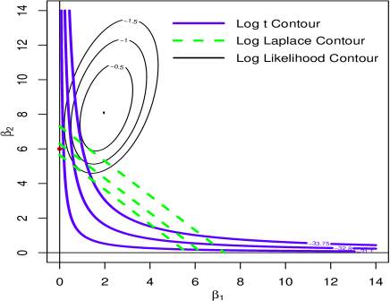
(a) Distinguishing Needles from hay

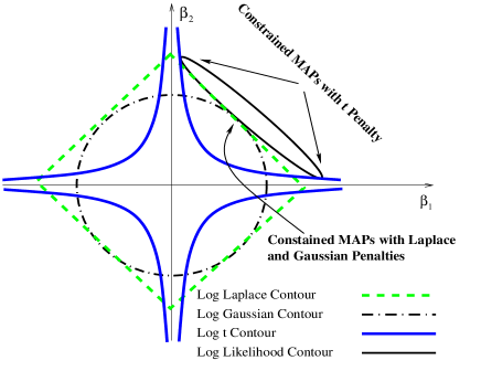
(b) Dividing Redundant Correlated Features

The ability of moderately hyper-LASSO priors to better separate “needles” from “hay” can be explained by looking at the “path” of constrained MAPs (maximizer of posterior) — the MAP with the log likelihood constrained to a particular value (i.e. on a contour). A constrained MAP can be found by shrinking the contour lines of log priors toward the origin until the two lines are tangent. Figure 1a shows three such constrained MAPs for a $t$ prior with df = 0.5 and $\sqrt{w}=e^{-10}$, and three for a Laplace prior based on a dataset generated with true coefficients $\beta_{1}=0,\beta_{2}=6,\beta_{0}=0$. The (unconstrained) MAP can then be found from the “path” containing these constrained MAPs. Because the contour lines of the log $t$ prior indent into the origin, the path of constrained MAPs based on the $t$ prior is flatter (with respect to x-axis) than the path based on Laplace; starting from the MLEs, the path based on the $t$ prior goes to a point at which $\beta_{1}$ is very close to 0 (but not exact 0), and $\beta_{2}$ is close to its true value (6), whereas, the path based on Laplace goes to the origin. Therefore we see that the $t$ prior can shrink small “hay” without much punishment to large “needles”.

From looking at constrained MAPs, we also find that hyper-LASSO penalties can automatically divide a group of correlated features into different posterior local modes. Figure 1b shows a conceptual illustration. When two features are highly correlated, a contour line of log likelihood is negatively correlated as shown in Figure 1b. With a $t$ penalty, the constrained MAPs are at the two ends of the contour of log likelihood, each of which uses only one of them to explain the class label without underestimating the importance of each of them. Therefore, the coefficients of highly correlated features are divided into different modes, each using only one of them. When the predictive abilities of the correlated features are different, the t prior can also make selections among a group of highly correlated features automatically. The selection within groups is necessary in high-dimensional problems in which a large group of correlated features often exists. By contrast, with Laplace and Gaussian penalties, the constrained MAPs are in the middle of the contour, favoring using all features with coefficients of smaller absolute values to explain the class label. When the group of correlated features is large, they may underestimate the absolute values of all of them, and hence, miss all of them, see a detailed discussion by Tolosi and Lengauer (2011a).

Figure 1b is also helpful for seeing that the primary computational difficulty of using hyper-LASSO priors in classification and regression problems is the presence of many local modes in the posterior distribution. An optimization algorithm can easily get trapped in a minor local mode arbitrarily depending on the initial values, so the algorithm becomes unstable and some sophisticated methods for choosing the initial values are required, see Griffin and Brown (2011).

3 Bayesian Logistic Regression with Hyper-LASSO Priors

We will now describe our method, BLRHL, including some technical details. Throughout this article, we will denote matrices with bold-faced letters, with row indexes displayed in the first subscript and column indices in the second. We denote real-valued vectors with bold-faced letters too, but with only a set of indices in subscript. The indices of matrices and vectors are denoted by $i\!:\!j$ — integers from $i$ to $j$, or a single integer for a row or column.

3.1 Multinomial Logistic Regression with Hyper-LASSO Priors

Suppose we have collected data of features and responses (class labels) on $n$ training cases. For a case indexed by $i$, we denote its class label by $y_{i}$, which can take integers $1,\ldots,C$, and denote $p$ features associated with it by a row vector $\mbox{\boldmath$x$}_{i,1:p}$. The hierarchical Bayesian multinomial logistic regression model used by us is described as follows:

$$P(y_{i}=c|\mbox{\boldmath$x$}_{i,1:p},\mbox{\boldmath$\beta$}_{0:p,1:C}) = \dfrac{\exp\left(\beta_{0,c}+\mbox{\boldmath$x$}_{i,1:p}\mbox{\boldmath$\beta$}_{1:p,c}\right)}{\sum_{c=1}^{C}\exp\left(\beta_{0,c}+\mbox{\boldmath$x$}_{i,1:p}\mbox{\boldmath$\beta$}_{1:p,c}\right)},\mbox{for }c=1,\ldots,C,$$ (2)

$$\mbox{\boldmath$\beta$}_{j,1:C}|\sigma_{j}^{2} \sim N\ (0,\sigma_{j}^{2}),\ \mbox{for }j=0,\ldots,p,$$ (3)

$$\sigma_{j}^{2} \sim \mbox{IG}\ (\alpha/2,w\alpha/2),\mbox{for }j=1,\ldots,p$$ (4)

where $\mbox{\boldmath$\beta$}_{0:p,1:C}$ are regression coefficients, and other variables are hyperparameters which are introduced to define the prior for $\mbox{\boldmath$\beta$}_{1:p,1:C}$ (and for convenience in MCMC sampling).

In this hierarchy, $\sigma_{j}^{2}$ indicates the importance of $j$th feature — the feature with larger $\sigma_{j}^{2}$ is more useful for predicting $y$, provided that all features are commensurable (which can be enforced by standardization). Note that we fix $\sigma_{0}^{2}$, not controlled by $w$, because we believe that the variability of intercepts is quite different from the variability of $\mbox{\boldmath$\beta$}_{j,1:C}$ for features. With $\mbox{\boldmath$\sigma$}^{2}_{1:p}$ marginalized with respect to IG prior (4), Equations (3) and (4) assign $\mbox{\boldmath$\beta$}_{j,1:C}$ ($j>0$) a $C$-dimensional $t$ prior with $\alpha$ degrees of freedom and $I_{C}\times\sqrt{w}$ as its covariance, whose PDF can be found from Kotz and Nadarajah (2004).

An important issue in multinomial logistic regression models is that the coefficients $\mbox{\boldmath$\beta$}_{j,1:C}$ are non-identifiable — if we add a constant to all $\mbox{\boldmath$\beta$}_{j,1:C}$, the conditional distribution of $y$ given $x$ in (2) is exactly the same. Therefore, the data can identify only the differences of $\mbox{\boldmath$\beta$}_{j,1:C}$ to a “baseline” class, say class 1, denoted by $\delta_{j,k}=\beta_{j,k+1}-\beta_{j,1}$, for $k=1,\ldots,C-1$. To avoid the non-identifiability problem, the coefficient for a baseline class, say $\beta_{j,1}$, is often fixed at 0, and $\mbox{\boldmath$\beta$}_{j,2:C}$ is assigned with a prior as in (3). However, such a prior is asymmetric for all classes: the prior variance of $\beta_{j,c}-\beta_{j,c^{\prime}}$ ($c,c^{\prime}\not=1$) double that of $\beta_{j,c}-\beta_{j,1}$. This implication may not be justified for practical problems. In addition, the feature selection can vary with the choice of baseline class.

We can use symmetric and identifiable parameters in multinomial logistic regression by transferring the symmetric prior for $\beta$’s to the identifiable parameters $\delta$’s. The identifiable parameters for model (2) are defined as:

$$\mbox{\boldmath$\delta$}_{j,k} = \mbox{\boldmath$\beta$}_{j,k+1}-\mbox{\boldmath$\beta$}_{j,1},\ \ \mbox{for }k=1,\ldots,\,\,K,\ \ j=0,\ldots,p,$$ (5)

where $K=C-1$. Note that $\delta_{j,k}$ is the coefficient associated with feature $j$ ($j=0$ representing intercept) and $y=k+1$. With $\delta_{j,k}$’s, the model (2) is now written as:

$$P(y_{i}=k+1|\mbox{\boldmath$x$}_{i,1:p},\mbox{\boldmath$\delta$}_{0:p,1:K}) = \dfrac{I(k=0)+I(k>0)\exp\left(\delta_{0k}+\mbox{\boldmath$x$}_{i,1:p}\mbox{\boldmath$\delta$}_{1:p,k}\right)}{1+\sum_{k=1}^{K}\exp\left(\delta_{0k}+\mbox{\boldmath$x$}_{i,1:p}\mbox{\boldmath$\delta$}_{1:p,k}\right)},$$ (6)

for $k=0,\ldots,K$, and $i=1,\ldots,n$.

We can transfer the symmetric prior for $\mbox{\boldmath$\beta$}_{j,1:C}$ to $\mbox{\boldmath$\delta$}_{j,1:K}$ rather than assigning independent priors for $\mbox{\boldmath$\delta$}_{j,1:K}$. Applying the standard transformation results for multivariate normal, the transformed parameters $\mbox{\boldmath$\delta$}_{j,1:K}$ are distributed with a joint multivariate Gaussian distribution:

$$\mbox{\boldmath$\delta$}_{j,1:K}|\sigma_{j}^{2}\sim N_{K}(\mbox{\boldmath$0$},(I_{K}+J_{K})\sigma_{j}^{2}),\mbox{for }j=0,\ldots,p,$$ (7)

where $I_{K}$ is a $K\!\times\!K$ identity matrix and $J_{K}$ is a $K\!\times\!K$ matrix with all elements 1. More explicitly, the joint PDF for (7) is given as follows:

$$P(\mbox{\boldmath$\delta$}_{j,1:K}|\sigma_{j}^{2}) = (2\pi\sigma_{j}^{2})^{-K/2}\exp\left(-\dfrac{V(\mbox{\boldmath$\delta$}_{j,1:K})}{2\sigma_{j}^{2}}\right)\times|I_{K}+J_{K}|^{-1/2},\mbox{where,}$$ (8)

$$V(\mbox{\boldmath$\delta$}_{j,1:K}) = \sum_{k=1}^{K}\delta_{jk}^{2}-\left(\sum_{k=1}^{K}\delta_{jk}\right)^{2}\Big{/}C.$$ (9)

Note that for $C=2$, (7) is just a univariate normal for $\delta_{j,1}$ with variance $2\sigma_{j}^{2}$.

We see that $V(\mbox{\boldmath$\delta$}_{j,1:K})$ in (9) is the sum of squared differences of $(\mbox{\boldmath$0$},\delta_{j,1},\ldots,\delta_{j,K})$ from its mean $(0+\sum_{k=1}^{K}\delta_{jk})/C$. $V(\mbox{\boldmath$\delta$}_{j,1:K})$ is exactly the same as the sum of squared differences of $\mbox{\boldmath$\beta$}_{j,1:C}$ to its mean, that is,

$$V(\mbox{\boldmath$\delta$}_{j,1:K})=\sum_{c=1}^{C}(\beta_{j,c}-\bar{\beta}_{j})^{2},\mbox{where }\bar{\beta}_{j}=(1/C)\sum_{c=1}^{C}\beta_{j,c},\mbox{ for }j=0,\ldots,p.$$ (10)

For feature selection, it is more straightforward to look at the standard deviation of $\mbox{\boldmath$\beta$}_{j,1:C}$, which is defined as a function of $\mbox{\boldmath$\delta$}_{j,1:K}$:

$$\mbox{SDB}(\mbox{\boldmath$\delta$}_{j,1:K})=\sqrt{V(\mbox{\boldmath$\delta$}_{j,1:K})/C},\mbox{for }j=0,\ldots,p$$ (11)

Note that when $C=2$, SDB$(\mbox{\boldmath$\delta$}_{j,1})=|\delta_{j,1}/2|$.

3.2 Horseshoe and NEG Priors

As alternatives to the Inverse-Gamma distribution in (4), other priors for $\sigma^{2}_{j}$ have been proposed in the recent literature for regression problems with the goal of shrinking $\mbox{\boldmath$\sigma$}_{j}^{2}$ associated with weak signal more towards 0. For example, Carvalho et al. (2010) proposed a horseshoe prior for coefficients by assigning a half (positive) Cauchy distribution for $\mbox{\boldmath$\sigma$}_{1:p}$. For uniformity of notation, we describe the half-Cauchy distribution using a half-t distribution with various degrees of freedom for $\sigma_{j}$, inducing the following prior for $\sigma_{j}^{2}$:

$$P_{ghs}(\sigma_{j}^{2})=\dfrac{\Gamma((\alpha+1)/2)}{\Gamma(\alpha/2)\sqrt{\alpha\pi}\sqrt{w}}\left(\dfrac{1}{1+\sigma_{j}^{2}/(\alpha w)}\right)^{\frac{\alpha+1}{2}}\,\dfrac{1}{(\sigma_{j}^{2})^{1/2}},\ \ \mbox{for }\sigma_{j}^{2}>0.$$ (12)

Griffin and Brown (2011) proposes using an NEG prior for coefficients by assigning an exp-gamma prior for $\sigma^{2}_{1:p}$: $\sigma_{j}^{2}|\psi_{j}\sim\exp(\frac{1}{\psi_{j}}),\psi_{j}\sim\mbox{IG}(\alpha/2,\alpha w/2)$, where $\psi_{j}$ is the mean parameter of exp distribution. We can marginalize $\psi_{j}$ and obtain a closed-form PDF for $\sigma_{j}^{2}$:

$$P_{neg}(\sigma_{j}^{2})=\dfrac{\kappa}{\lambda}\left(\dfrac{1}{1+\sigma_{j}^{2}/\lambda}\right)^{\alpha/2+1},\ \ \mbox{for }\sigma_{j}^{2}>0$$ (13)

where $\kappa=\alpha/2$ and $\lambda=\alpha w/2$ for notational simplicity. We will call (12) and (13) the GHS and NEG priors for $\sigma_{j}^{2}$. Note that these names are also used for the priors of the coefficients $\mbox{\boldmath$\delta$}_{j,1:K}$ when $\sigma_{j}$ integrated out. The PDFs of GHS and NEG priors for $\sigma_{j}^{2}$ do not converge to $0$ as $\sigma_{j}^{2}$ goes to $0$ (as the IG prior does); therefore it is possible that regression coefficients are better shrunken towards $0$ without punishing large signals. This property is indeed desired, and may be beneficial. However, our numerical experiments show that using these two priors over a $t$ prior makes little difference in MCMC inference. Additionally, adaptive rejection sampling (Gilks and Wild, 1992) (or other sampling methods) for the posteriors of $\sigma_{j}^{2}$ given $\mbox{\boldmath$\beta$}_{j,1:C}$ based on GHS and NEG priors is needed in Gibbs sampling. By contrast, direct sampling for $\sigma_{j}$ is available if IG is used. This additional sampling could significantly increase the total MCMC sampling time when $p$ is large.

Choosing the scale $\sqrt{w}$ is an important issue for any inference with shrinkage. However, when $\alpha=1$, we recommend to fix $w$ around a reasonable value, e.g. $\log(w)=-10$. Most random numbers generated by $t$/GHS/NEG distributions with this setting are very small, but contain a fairly large portion of values between 0 and 2, which can model a wide range of problems. Our following empirical results will show that when $\alpha=1$, the fitting results are not sensitive to the choice of small $w$. When $\alpha>1$, it is better to treat the scale as a hyperparameter assigned with a prior; this is because the results are sensitive to $\sqrt{w}$. In our implementation, we assign a vague normal prior for $\log(w)$.

3.3 Gibbs Sampling Procedure

We use a Gibbs sampling procedure to sample the full posterior distribution of BLRHL model. The full posterior distribution is written as:

$$P(\mbox{\boldmath$\delta$}_{0:p,1:K},\mbox{\boldmath$\sigma$}_{1:p}^{2}|\mbox{\boldmath$D$})\propto L(\mbox{\boldmath$\delta$}_{0:p,1:K})\times P(\mbox{\boldmath$\delta$}_{0:p,1:K}|\mbox{\boldmath$\sigma$}_{0:p}^{2})\times P\left(\mbox{\boldmath$\sigma$}_{1:p}^{2}\,|\,\alpha/2,\alpha\,w/2\right),$$ (14)

where $D$ represents the data $y_{i},\mbox{\boldmath$x$}_{i,1:p}$ for $i=1,\ldots,p$ and other fixed values in BLRHL models — $\alpha,\sigma_{0}^{2}$; $L$ is the likelihood function: $L(\mbox{\boldmath$\delta$}_{0:p,1:K})=\prod_{i=1}^{n}P(y_{i}|\mbox{\boldmath$x$}_{i,1:p},\mbox{\boldmath$\delta$}_{0:p,1:K});$ the last two parts are the PDFs of priors specified by (7), and one of the priors given in (4), (12), or (13). We sample the full posterior in (14) by sampling the conditional distribution of $\mbox{\boldmath$\sigma$}_{1:p}^{2}$ and $\mbox{\boldmath$\delta$}_{0:p,1:K}$ given each other alternately for a number of iterations. If IG prior (4) is used, the Gibbs sampling procedure involves alternating the following two steps:

• Given $\mbox{\boldmath$\sigma$}_{1:p}^{2}$ fixed, update $\mbox{\boldmath$\delta$}_{0:p,1:K}$ jointly with a Hamiltonian Monte Carlo transformation that leaves invariant the following distribution:

  $$P(\mbox{\boldmath$\delta$}_{0:p,1:K}|\mbox{\boldmath$\sigma$}_{0:p}^{2},\mbox{\boldmath$D$})\propto L(\mbox{\boldmath$\delta$}_{0:p,1:K})\times P(\mbox{\boldmath$\delta$}_{0:p,1:K}|\mbox{\boldmath$\sigma$}_{0:p}^{2}).$$ (15)

• Given value of $\mbox{\boldmath$\delta$}_{1:p,1:K}$ from Step 1, update $\mbox{\boldmath$\sigma$}_{1:p}^{2}$ by sampling from

  $$\sigma_{j}^{2}|\mbox{\boldmath$\delta$}_{j,1:K} \sim \mbox{IG}\left(\sigma_{j}^{2}\,\Big{|}\,\frac{\alpha+K}{2},\frac{\alpha w+V(\mbox{\boldmath$\delta$}_{j,1:K})}{2}\right),\mbox{for }j=1,\ldots,p$$ (16)

Note that in Step 2, $\sigma^{2}_{0}$ is opted out of the updating process as it is fixed at a large value. The sampling for (16) in Step 2 is straightforward; when Horseshoe and NEG priors are used, the sampling method for Step 1 can be the same, but we have to use the posterior of $\sigma_{j}^{2}$ given $\mbox{\boldmath$\delta$}_{j,1:K}$ differently in Step 2. When we use GHS prior (12) for $\sigma_{j}^{2}$, the conditional posterior of $\sigma^{2}_{j}$ given $\mbox{\boldmath$\delta$}_{j:1:K}$ [instead of Equation (16)] is:

$$P_{ghs}(\sigma_{j}^{2}|\mbox{\boldmath$\delta$}_{j,1:K})\propto\dfrac{1}{(\sigma_{j}^{2})^{K/2}}\,\exp\left(-\dfrac{V(\mbox{\boldmath$\delta$}_{j,1:K})}{2\sigma_{j}^{2}}\right)\times\left(\dfrac{1}{1+\sigma_{j}^{2}/(\alpha w)}\right)^{\frac{\alpha+1}{2}}\,\dfrac{1}{(\sigma_{j}^{2})^{1/2}}.$$ (17)

The induced conditional distribution for $\xi_{j}=\log(\sigma^{2}_{j})$ from the above distribution is log-concave and can be sampled with ARS (Gilks and Wild, 1992). When we use an NEG prior (13) for $\sigma_{j}^{2}$, the conditional posterior of $\sigma^{2}_{j}$ given $\mbox{\boldmath$\delta$}_{j,1:K}$ [instead of Equation (16)] is

$$P_{neg}(\sigma_{j}^{2}|\mbox{\boldmath$\delta$}_{j,1:K})\propto\dfrac{1}{(\sigma_{j}^{2})^{K/2}}\,\exp\left(-\dfrac{V(\mbox{\boldmath$\delta$}_{j,1:K})}{2\sigma_{j}^{2}}\right)\times\left(\dfrac{1}{1+\sigma_{j}^{2}/\lambda}\right)^{\alpha/2+1}.$$ (18)

The induced posterior of the log transformation $\xi_{j}=\log(\sigma_{j}^{2})$ from the above distribution is log-concave and can be sampled with ARS.

The key component in the above procedure is the use of Hamiltonian Monte Carlo (HMC) for updating high-dimensional $\mbox{\boldmath$\delta$}_{0:p,1:K}$. In Section A.2 we give a concise description of HMC; this method can greatly suppress the random walk due to correlation (which is common in logistic regression posteriors; see our real data examples) with a long leapfrog trajectory (Neal, 2010). The major problem of sampling from posteriors based on hyper-LASSO priors is the existence of many local modes due to feature redundancy. Applying HMC in the above Gibbs sampling framework can travel across the modes fairly well for the following reason. When both $\sigma^{2}_{j}$ for two correlated features are large, the joint conditional distribution of their coefficients given $\sigma_{j}^{2}$ in Step 1 is highly correlated, probably close to their likelihood function as shown in Figure 1b. Because a fairly long HMC trajectory has a much greater chance than ordinary MCMC methods to move from one end of the contour to the other end, the Markov chain can travel from one mode to another. For high-dimensional problems with very large $p$, such as thousands, Step 1 is computationally intensive as it involves updating $p*K$ coefficients in each step. This challenge can be relieved greatly by an important trick that we call “restricted Gibbs sampling”, where only the coefficients with $\sigma_{j}^{2}$ greater than a certain threshold are updated in Step 1. The details of this trick are given in Section A. A list of notations for the settings of BLRHL is given in Section B.

3.4 Feature Importance Measures from Markov chain Samples

With posterior samples of $\mbox{\boldmath$\delta$}_{1:p,1:K}$, we recommend using means over iterations to estimate the coefficients (these estimates are denoted by $\hat{\delta}_{j,1:K}$). We then compute SDB($\hat{\mbox{\boldmath$\delta$}}_{j,1:K})$ using formula (11) to obtain an importance measure for feature $j$; these features can then be ranked by SDB($\hat{\mbox{\boldmath$\delta$}}_{j,1:K})$. As we have discussed in Section 2, the Markov chain sample pool is a mixture of subpools from different modes, each corresponding to a succinct feature subset. Thus, the mean over the Markov chain is a summary of the importance of the feature, not an estimate of the true coefficient. However, this method omits some useful features that appear with low frequency in Markov chain samples. In the context of high-dimensional problems, there are often a large number of such correlated features, therefore, discriminating them according to their predictive ability is desired. The ranking by means can omit many correlated features with weaker predictive ability as well as those totally useless, hence pinning down a very small subset of highly relevant features.

4 Simulation Studies

4.1 Comparing Scaling Effects in LASSO and Hyper-LASSO

We generated a dataset of $n=1100$ cases (of which 100 were used for fitting models and the other 1000 were used to look at predictive performance) and $p=200$ features, where the response $y_{i}$ is equally likely to be 1 and 2. Given $y_{i}$, 200 features are generated from the following Gaussian models:

$$x_{1}|y=c = \mu_{c}+z_{1}+\epsilon_{1},$$ (19)

$$x_{2}|y=c = 2z_{1}+z_{2}+\epsilon_{2},$$ (20)

$$x_{j}|y=c = \epsilon_{j},\mbox{ for }j=3,\ldots,200$$ (21)

where $\mu_{1}=0,\mu_{2}=2$ and $z_{1},z_{2},\epsilon_{j}$ are all distributed as $N(0,1)$. In this model, only the first feature is differentiated across two classes, and the 2nd is non-differentiated but correlated with the 1st; therefore only the first two features are useful for predicting the response $y$. Using Bayes rule, we can find the conditional distribution of $y$ given $x$; this distribution is a logistic regression model with true coefficients $\mbox{\boldmath$\delta$}_{0:2,1}=(0,2.60,-1.22)$ and others equal to $0$. The relationship between $y$ and $x$ is simple, but the signals are placed among the other 198 unrelated features. Figure 2 shows the scatterplots of the 2nd and 3rd features to the 1st with shapes representing the two classes.

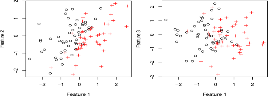
Figure 2: Scatterplots of the first three features from a simulated dataset used in Section 4.1.

We ran BLRHL that uses a t prior with $\alpha=1$ and MCMC settings as follows: $n_{1}=50K,\ell_{1}=5,n_{2}=100K,l_{2}=50,\epsilon=0.3,\zeta=0$, and 100 different $\log(w)$ spaced evenly from $-24$ to $-8$. The meanings of these setting parameters are listed in Section B. For each choice of scale, we estimated the coefficients using means of Markov chain samples. These results allow us to draw the solution paths (Figure LABEL:fig:p200pathes) of all the coefficients against the log of the scale and compare the path given by LASSO (using R package glmnet). We can see that BLRHL gives much more distinctive estimates of the two non-zero coefficients from those of the other 198 useless features than LASSO. Due to the inclusion of many useless features, LASSO cannot identify the second feature distinctively. From comparing these paths, we also see that the estimates by BLRHL are very stable for the choices of $w$ in a very wide range. There is an upward bias in the mean estimates when $\sqrt{w}$ is large; this is because the marginal posterior distributions of the two coefficients for two correlated features are skewed to large absolute values. This bias, however, does not affect the predictive performance and feature selection.

Figure LABEL:fig:p200predpath shows the predictive performance of BLRHL and LASSO measured by AMLP — the average minus log predictive probabilities at the true labels. The AMLP paths are shown in Figure LABEL:fig:p200predpath. We see that BLRHL predicts better than LASSO; more importantly, the predictive performance of BLRHL is very stable for a wide range of $\sqrt{w}$. By contrast, LASSO is very sensitive to the choice of $\sqrt{w}$.

Figure 3: Comparison of coefficient estimates and AMLPs against log scale for the study in Section 4.1. The numbers on the top of LABEL:fig:p200pathes show the number of coefficients with absolute values not smaller than 0.1 times the maximum value in all coefficients.

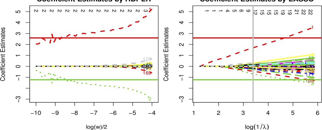
(a)

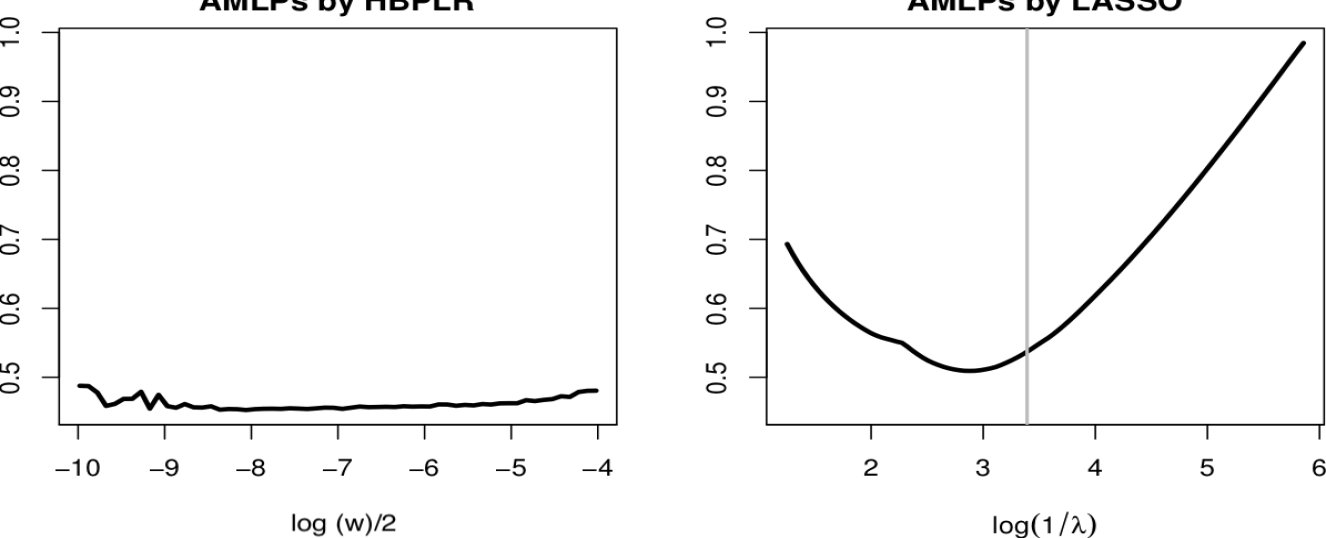
(b)

4.2 Investigating the Choice of Heaviness ($\alpha$)

We generated 50 datasets ($n=2100$ cases, $100$ of which was used for training, while the other 2000 were used to test predictions) as follows. The number of classes $C$ is set to 3, and class labels are equally likely drawn from 1, 2, and 3. The first two features were generated in a similar way as the $x_{1}$ and $x_{2}$ of the dataset used in Section 4.1, with an addition of class $3$ having $0$ for means. We add another group of features ($x_{3}-x_{10}$) that are highly correlated within groups but are independent of $x_{1}$ and $x_{2}$, and have mean equal to 2 in class 3. More specifically, values of these 10 features for each case were generated as follows:
$\displaystyle x_{1}|y=c$ $\displaystyle=$ $\displaystyle\mu_{c,1}+z_{1}+0.5\epsilon_{1},$ $\displaystyle x_{2}|y=c$ $\displaystyle=$ $\displaystyle\mu_{c,2}+2z_{1}+z_{2}+0.5\epsilon_{2},$ $\displaystyle x_{j}|y=c$ $\displaystyle=$ $\displaystyle\mu_{c,j}+z_{3}+0.5\epsilon_{j},\ \mbox{for }j=3,\ldots,10,$

$$\mbox{where }(\mu_{c,j})_{3\times 10}=\left(\begin{array}[]{ccccc}0&0&0&\ldots&0\\ 2&0&0&\ldots&0\\ 0&0&2&\ldots&2\end{array}\right),$$

and $z_{j}$ and $\epsilon_{j}$ are independently generated from $N(0,1)$. In addition to these 10 features, we also attached 1990 features simply drawn from N(0,1), which we will call absolute “hay”. In this model, $x_{1}$ is differentiated with a different mean in class 2 from classes 1 and 3. $x_{2}$ is non-differentiated, but correlated with $x_{1}$ and therefore is useful, as shown by Figure 2. $x_{3}-x_{10}$ are all differentiated, with different means in class 3 from classes 1 and 2. However $x_{3}-x_{10}$, which have the same class means and are related to a common factor $z_{3}$, are highly correlated and redundant for predicting $y$; we will refer to this group as “correlated features”.

We ran BLRHL using t priors with 4 choices of $\alpha$: 0.2, 0.5, 1, 4, 10; the setting for $\log(w)$ varies slightly for different $\alpha$. When $\alpha=1$, we chose two values of $\log(w)$: -20 and -10. When $\alpha=4$ and 10, we chose to treat $\log(w)$ as a hyperparameter assigned with a normal prior with variance 100 (this is because for large $\alpha$, the results for feature selection and prediction are sensitive to the choices of scale and we therefore show the results with $\log(w)$ chosen automatically during MCMC simulation). The values of $\log(w)$ for $\alpha=0.2/0.5$ are -40/-20 respectively. For setting MCMC, when $\alpha=1$, we chose $n_{1}=50K,\ell_{1}=10,n_{2}=500K,\ell_{2}=50,\epsilon=0.3,\zeta=0.05$. The details of these setting parameters can be found in Appendix B. In particular we have run MCMC for various choices of $\zeta$ in restricted Gibbs sampling for a given dataset; the results are fairly stable. When $\alpha$ equals to 0.2/0.5/4/10 (other than 1), we set a larger $n_{2}=1M$ for the longer chain, with the other settings being the same as the $\alpha=1$ case. We ran BLRHL using GHS and NEG priors with settings $\alpha=1$ and $\log(w)=-10$, and the same other settings for running BLRHL using a t prior with $\alpha=1$. We ran LASSO with $\lambda$ chosen by cross-validated AMLP.

Figure 4: SDBs given by BLRHL methods and LASSO on a synthetic dataset with $p=2000$ features. The red numbers show the indices of top features with relative SDB greater than 0.1, except for (4b) which shows indices of features with relative SDB greater than 0.5 (to avoid showing too many indices). The horizontal lines indicate the values equal to 0.1 and 0.01 times the maximum SDB. The x-axis is in log-scale in order to better look at signal features.

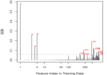
(a) SDBs of LASSO

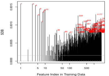
(b) SDBs of BLRHL with $t(\mbox{df}=10)$

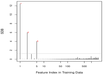
(c) SDBs of BLRHL with $t(\mbox{df}=1,\log(w)=-10)$

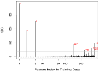
(d) SDBs of BLRHL with $t(\mbox{df}=0.2,\log(w)=-40.0)$

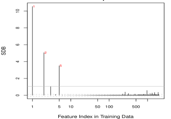
(e) SDBs of BLRHL with $\mbox{NEG}(\mbox{df}=1,\log(w)=-10)$

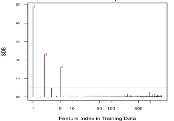
(f) SDBs of BLRHL with $\mbox{GHS}(\mbox{df}=1,\log(w)=-10)$

We first look at the coefficient shrinkage effects of hyper-LASSO priors with different $\alpha$ and LASSO. Figures 4 show the SDBs of all 2000 features from the dataset. From Figure 4, we see that BLRHL methods using t/GHS/NEG priors with $\alpha=1$ perform feature selection very well. First, they can distinctively separate the absolute “hay” from other useful features. Second, they do not miss the 2nd feature which is useful but has weaker relevance. Third, they rank highly one feature ($x_{5}$) from the 8 correlated features, recognize another feature $x_{3}$ as useful too, and suppress others. By contrast, when $\alpha$ is large (e.g. 10), we see that the LASSO and BLRHL methods: 1) cannot separate the absolute “hay” distinctively from the few “needles”; 2) miss $x_{2}$ for this dataset (and very often for other datasets), which we think is because they include too much “hay” and overfit the data, making $x_{2}$ harder to identify; 3) tend to include many of the correlated features into their unique mode without clear discrimination for importance. BLRHL with very small $\alpha=0.2$ (very heavy tails) can do feature selection well, but their overly flat tails allow the “needles” to go to very large values (such as thousands, see Figure 4d), resulting in very poor prediction in some cases. To summarize the performance of feature selection, we cut SDBs by 0.1 times the maximum SDB (i.e., by thresholding relative SDBs with 0.1). Table 2 shows the averages of numbers of retained features in each of the 4 different groups. BLRHL with 10 degrees of freedom selects significantly more noise features; this is because the SDBs of all features are very close due to the light tail (as shown by Figure 4b). Table 2 confirms the above observations about the effects of priors with different heaviness in coefficient shrinkage. The choice of 0.1 as a threshold is an ad-hoc choice; the comparison of feature selection performance between different priors is very similar for different thresholds used to cut the SDBs — Section 4.3 presents the feature selection results against a set of choice of thresholds ranging from 0.01 to 0.2 using 500 datasets.

Table 2: Means of numbers of retained features by thresholding relative SDBs with 0.1 in different groups in 50 datasets. Numbers in brackets show the standard deviations of the 50 numbers.

	Groups of Features
Methods	$x_{1}$	$x_{2}$	$x_{3}-x_{10}$	$x_{11}-x_{2000}$
LASSO	1	0.34	2.72 (1.18)	6.92 (4.97)
BLRHL with t (df=10)	0.96	0.66	7.42 (1.86)	1354 (580)
BLRHL with t (df=4)	1	0.36	1.26 (0.53)	0.00 (0.00)
BLRHL with t (df=1,$\log(w)=-20$)	1	0.94	1.14 (0.35)	0.16 (0.37)
BLRHL with t (df=1,$\log(w)=-10$)	1	0.96	1.10 (0.30)	0.32 (0.55)
BLRHL with GHS (df=1,$\log(w)=-10$)	1	1.00	1.14 (0.35)	0.30 (0.51)
BLRHL with NEG (df=1,$\log(w)=-10$)	1	1.00	1.06 (0.24)	0.28 (0.50)
BLRHL with t (df=0.5,$\log(w)=-20$)	1	0.98	1.16 (0.37)	1.14 (0.97)
BLRHL with t (df=0.2,$\log(w)=-40$)	1	0.72	1.36 (0.60)	5.74 (3.12)

Figure 5 shows boxplots of the 50 AMLPs for each method on 2000 test cases. From these plots, we see that BLRHL (using t/GHS/NEG priors) with $\alpha=1$ gives substantially better predictions for most of the datasets than the other choices of $\alpha$ (as well as LASSO). LASSO and BLRHL with very large and very small $\alpha$ do not predict well. Note that the AMLPs of all runs with $\alpha=0.2$ are infinity; these are not shown in Figure 5. Therefore, the choice of $\alpha$ is critical for BLRHL to work well for high-dimensional classification, and $\alpha=1$ is recommended based on our investigation in these simulated datasets with super-sparse signals.

Figure 5: Boxplots of AMLPs for 2000 test cases using BLRHL with various priors, and LASSO. “df” in the plot represents the choice of $\alpha$ for BLRHL priors.

4.3 Evaluation of BLRHL with 500 Simulated Datasets

We generated 500 datasets (in the same way as described in Section 4.2) to evaluate BLRHL more intensively. We apply BLRHL to these datasets using $t$/GHS/NEG priors with $\alpha=1,\log(w)=-10$ (the optimal choice from the previous investigation), and the same other MCMC settings and compared them to LASSO.

For each dataset, we perform feature selection by cutting the relative SDBs produced by each method for each dataset using 15 values evenly spaced between 0.01 and 0.2. At each threshold, we calculate the number of retained features, false positive false rate (FPR), sensitivity (proportion of useful features included), and false discovery rate (FDR). FDR is defined as the proportion of unrelated features within retained features. In calculating sensitivity, we treat the features in group 3 (i.e., $x_{3}$ to $x_{10}$) as a single useful feature. We average the previous four measures over 500 datasets, with results shown in Figure 6. Clearly, we see that BLRHL methods retain much smaller feature subsets with the same threshold compared to LASSO. We also see that BLRHL has higher sensitivities, lower FPRs, and lower FDRs than LASSO. The high FPRs and FDRs of LASSO result from the inclusion of many unrelated features. Additionally, Figure 6 indicates that horseshoe and NEG priors have slightly lower FDRs than the $t$ prior.

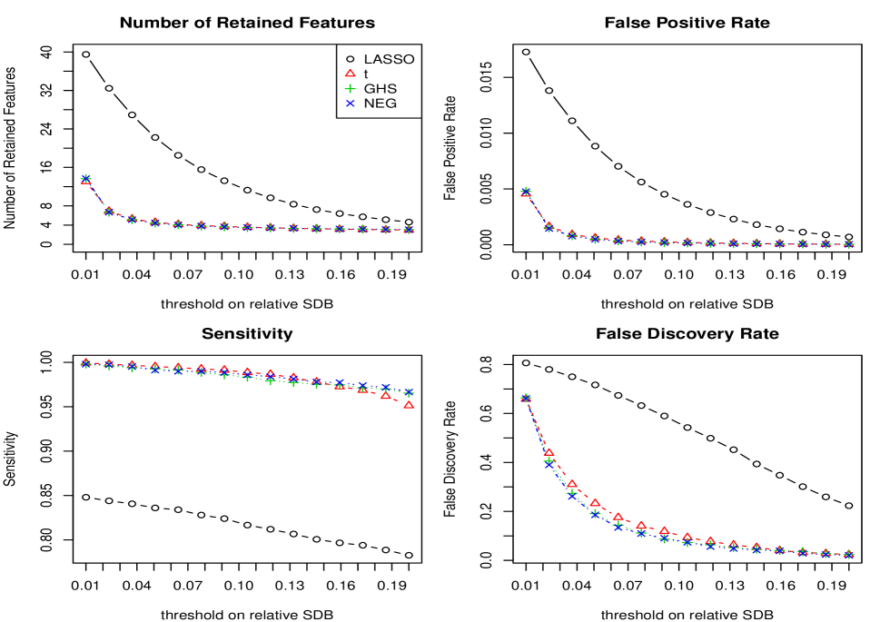
Figure 6: Comparison of feature selection with 500 datasets

To compare predictive performance, we collect the AMLPs over 500 datasets for each method. The comparative boxplots of the AMLPs for the four methods is shown in Figure 7a. We see that BLRHL based on different priors with the same $\alpha=1$ achieves significantly lower AMLPs than LASSO and performs very similarly with each other. In order to account for the different predictive difficulties in the 500 datasets, we calculated the percentage of AMLP reduction of each BLRHL method relative to the AMLP of LASSO for each dataset (shown in Figure 7b). From this Figure we see that the predictive accuracies of the BLRHL methods are about 30% higher than LASSO for the majority of these 500 datasets.

Figure 7: Comparison of predictive performance with 500 datasets. (a) shows the AMLP boxplots for each method; the top line shows the expected AMLP ($\log(3)$) when one makes random prediction. (b) shows the box plots of percentages of AMLP reductions in comparing BLRHL to the LASSO.

(a) AMLPs

(b) Percentages of AMLP Reduction

5 Application to a Prostate Microarray Dataset

We applied BLRHL to a real microarray gene expression data that is related to prostate cancer; this dataset has expression profiles for 6033 genes from 50 normal and 52 cancerous tissues, and was originally reported by Singh et al. (2002). We analyzed a dataset downloaded from the website http://stat.ethz.ch/~dettling/bagboost.html for Dettling (2004), which contains more descriptions about this dataset. To improve the visualization of our results, we re-ordered the features by their F-statistics on the whole dataset; therefore the indices of the genes discussed below are also the ranks of features according to their F-statistics. We ran BLRHL using t/GHS/NEG priors and LASSO with $\lambda$ chosen with cross-validation in training cases. Before fitting with BLRHL, we standardized the features solely with training data (LASSO does such standardization as well). We ran BLRHL with the following settings for each of the 6033 genes: $\alpha=1,\log(w)=-10,n_{1}=100K,\ell_{1}=10,n_{2}=1M,\ell_{2}=50,\epsilon=0.3,\zeta=0.05$. Each Markov chain took about 10 hours if a t prior was used, and about 33 hours if GHS/NEG priors were used.

We use leave-one-out cross-validation (LOOCV) to obtain the predictive probabilities for each of the methods considered here. One advantage of LOOCV is that the number of training cases is only one less than the sample size in the whole dataset; therefore LOOCV predictive measures are believed to be the closest to the out-of-sample predictions based on the whole dataset. Figure 8d shows the SDBs of BLRHL and LASSO when the 2nd case was left out as a test case and the remaining cases were used as training. The 2nd case was chosen to present in this article without any particular reason, as the results are similar for each case left out. P-values given by the F-statistic are calculated for all 102 cases. Figure 8d shows the results of rerunning BLRHL using a t prior on only the top 50 genes selected using the run with all 6033 genes. The results for BLRHL using the Horseshoe and NEG priors are nearly the same as using the $t$ prior; for this reason they are not shown here. These plots show that BLRHL methods distinctively select fewer than 10 genes by thresholding relative SDBs with 0.01. The F-statistic ranks more than 1000 genes with p-values smaller than 0.01; these genes are actually highly correlated and contain redundant information, therefore they are omitted by BLRHL. We note that, except for gene 1, all other top genes selected by BLRHL have very low F-statistic ranks (e.g. genes 369, 977 and 2866 — recall that the index is just the F-statistic rank). We see that LASSO gives many non-zero but small SDBs greater than the value of 0.01 times the maximum SDB, hence LASSO includes many more genes than BLRHL. However, we notice that LASSO omits gene 977, which is ranked the 3rd by BLRHL (later we will use cross-validation to show that this gene is indeed important).

Figure 8: Gene selection results on prostate data using different methods. For LASSO and BLRHL, the red numbers under points show the indices of ranked genes by their F-statistic, and the horizontal lines indicate the values equal to 0.1 and 0.01 times the maximum SDB. The red numbers show indices of genes selected by thresholding relative SDBs with 0.01. For p-values, the lines indicates -log(0.05) and -log(0.01). The x-axis is in log-scale to better highlight the top genes as selected by the F-statistic rank.

(a) -log(p-values) given by F-statistic

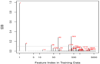
(b) SDBs of LASSO

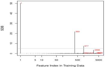
(c) SDBs of BLRHL with $t(\mbox{df}=1,\log(w)=-10)$

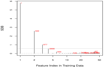
(d) SDBs from rerunning BLRHL for top 50 Genes

Table 3 shows LOOCV predictive performances measured by AMLP and error rate. In this table we have also included the results of six other methods reported by Dettling (2004). We see that BLRHL methods are substantially better than many other methods; compared to LASSO, BLRt gains 47% reduction in AMLP.

Table 3: Comparison of LOOCV predictive performances of BLRHL and others. BLRt, BLRghs and BLRneg are BLRHL using t, GHS and NEG priors respectively.

Methods	BLRt	BLRghs	BLRneg	LASSO	Bagboost	PAM	DLDA	SVM	RanFor	kNN
AMLP	.156	.158	.152	.274	-	-	-	-	-	-
ER (%)	6.86	7.84	7.84	10.8	7.53	16.5	14.2	7.88	9.00	10.59

Figure 9 shows the scatterplots of log predictive probabilities at the true class labels for BLRHL and LASSO. The difference in AMLPs between BLRHL (using a t prior) and LASSO is statistically significant, with a p-value of $4.6\times 10^{-4}$ calculated using a paired one-sided t test. The performances of BLRHL using t/GHS/NEG priors are nearly the same, as shown by Figure 9b.

Figure 9: Comparisons of log predictive probabilities at true class labels.

(a) BLRHL vs LASSO

(b) $t$ vs NEG

To assess the gene selection results of BLRHL, Figure 10c shows some scatterplots of the top ranking genes (1,369,977,2866). From these plots we see that genes 369, 977, and 2866 are weakly differentiated across two classes but are useful because they are correlated with the most differentiated gene 1. Gene 2866 is ranked lower because it is correlated with gene 977 as shown by Figure 10b. Figure 10c show that the combination of genes 1, 369 and 977 provides a clear separation for the normal and cancerous tissues.

Figure 10: Scatterplots of some top genes selected by BLRHL. The two red numbers or + in 10c label the two cases misclassified in LOOCV.

(a)

(b)

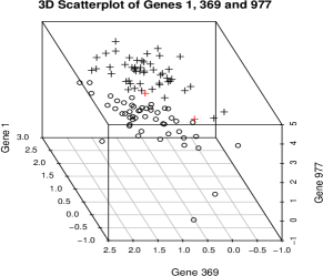
(c)

We further compare the top 3 genes found by BLRHL with other small gene subsets by looking at their LOOCV predictive power. We reran BLRHL (using t priors with $\alpha=1$) on the dataset containing only genes of a fixed subset (in LOOCV fashion) in order to obtain the predictive power of the given gene subset; these results are shown in Table 4. The subset of genes 1, 369 and 977 is substantially better than other subsets in separating the two classes; this is confirmed by the 3D scatterplots (Figure 10c) of the top 3 genes. We think that the subset of genes 1, 369, and 977 is worthy of further biological investigations. From Table 4, we also see that gene 977 (which is omitted by LASSO) is indeed useful because the subset of genes 1, 369 and 977 has significantly better predictive power than the subset containing only genes 1 and 369; the AMLP is reduced from 0.232 to 0.05 after including gene 977, with a reduction percentage of $78\%$. By contrast, the third gene selected by LASSO (gene 83) does not reduce AMLP as much as gene 977.

Table 4: LOOCV predictive performances of various gene subsets.

Gene subset	1, 369, 977	1, 369	1, 2, 3	1, 369, 83
Selected by	BLRHL	BLRHL and LASSO	F-Statistic	LASSO
AMLP	.050	.232	.240	.163
ER (%)	1.96	8.82	9.80	7.84

6 Conclusions and Discussions

In this article we have introduced an MCMC (fully Bayesian) method for learning severely multi-modal posteriors of logistic regression models based on hyper-LASSO priors (non-convex penalties). With empirical studies, we have shown that our MCMC algorithm can effectively explore the multi-modal posterior, and hence achieves superior out-of-sample predictive performance and desired hyper-LASSO sparsity for feature selection. Our empirical studies have also demonstrated two important facts about the choice of heaviness and scale of hyper-LASSO priors for logistic regression in datasets with super-sparse signals. First, the choice of the degrees of freedom that control tail heaviness should be appropriate; priors with tail heaviness similar to Cauchy appear optimal. Second, due to the “flatness” in the tails of Cauchy, the shrinkage of large coefficients is very small (i.e. small bias); more importantly, the shrinkage is very robust to the choice of scale, which is a distinctive property of Cauchy priors (compared to Laplace and Gaussian priors). In particular, the choice of $-10$ used in this article for the log scale of Cauchy is expected to work well for a wide range of problems with features standardized to have a standard deviation close to 1, e.g. binary indicator variables derived from categorical variables.

In light of the fact that the posterior distributions based on hyper-LASSO priors are severely multi-modal, summarizing the feature importance by averaging the coefficients over all modes may not the best choice. In particular, when there is a large group of highly correlated features, many features in the group will be selected when using the means of coefficients. A more sophisticated method for interpreting the fitting results is to use a clustering algorithm to divide the whole Markov chain samples into subpools, look at the subpools separately, and then deliver a list of succinct feature subsets. If one can split Markov chain iterations as this, it will then be better to use the median to obtain an importance index, as it can better shrink the coefficients of totally useless features towards $0$ and correct for the skewness of the posterior. This will demand further development of methods for interpreting the MCMC samples from a multi-modal posterior. Another very interesting method is to find a feature subset from the MCMC samples that have the best matching (not the best training predictive power) to the full MCMC samples using the so-called reference/projection approach (Goutis and Robert, 1998; Dupuis and Robert, 2003; Piironen and Vehtari, 2017).

Appendices

Appendix A Computational Method for BLRHL

This section is a continued discussion from Section 3.3 about our computational method.

A.1 Initial Values for Gibbs Sampling

The initial values for $\delta_{0:p,1:K}$ are coefficients of the Bayes discriminant rule based on Gaussian distributions whose mean vectors are estimated by the medians of Markov chain samples produced by the method described in Li (2012) and whose covariance matrix is estimated by an equally weighted average of the sample covariance and the identity matrix.

A.2 Updating $\delta_{0:p,1:K}$ with Hamiltonian Monte Carlo

Suppose that we want to sample from a $d$-dimensional distribution with PDF proportional to $\exp(-U(\mbox{\boldmath$q$}))$ , or construct a transformation leaving it invariant. For our problem, $U(\mbox{\boldmath$q$})$ is the minus log of the posterior distribution of $\mbox{\boldmath$q$}=\mbox{\boldmath$\delta$}_{0:p,1:K}$ (i.e. the minus log of (15)).

We will augment $q$ with a set of auxiliary variables $p$ that are independently distributed with $N(0,1)$ and are independent of $q$. For this purpose we will randomly draw a $p$ independently from $N(0,1)$. In physics, $p$ is interpreted as momentum’s of particles. Next we will transform $(\mbox{\boldmath$q$},\mbox{\boldmath$p$})$ in a way that leaves invariant $\exp(H(\mbox{\boldmath$q$},\mbox{\boldmath$p$}))$ — the joint distribution of $(\mbox{\boldmath$q$},\mbox{\boldmath$p$})$, where $H(\mbox{\boldmath$q$},\mbox{\boldmath$p$})$ is often called Hamiltonian, which is given by:

$$H(\mbox{\boldmath$q$},\mbox{\boldmath$p$})=U(\mbox{\boldmath$q$})+K(\mbox{\boldmath$p$})=U(\mbox{\boldmath$q$})+\frac{1}{2}\sum_{i=1}^{d}p_{i}^{2}.$$

At the end of this transformation, we will discard $q$, obtaining a new $p$ that is still distributed with $\exp(-U(\mbox{\boldmath$p$}))$.

The method for transforming $(\mbox{\boldmath$q$},\mbox{\boldmath$p$})$ is inspired by Hamiltonian dynamics, in which $(\mbox{\boldmath$q$},\mbox{\boldmath$p$})$ moves along a continuous time $\tau$ according to the following differential equations:

$$\frac{dq_{i}(\tau)}{d\tau} = \frac{\partial H}{\partial p_{i}}\ \ \ =\ \ \ \frac{\partial K}{\partial p_{i}}\ \ \ =\ \ \ p_{i}$$

$$\frac{dp_{i}(\tau)}{d\tau} = -\frac{\partial H}{\partial q_{i}}\ \ \ =\ \ \ -\frac{\partial U}{\partial q_{i}}$$

It can be shown that this Hamiltonian dynamic keeps $H$ unchanged and preserves volume (see details from Neal (2010)). These are the crucial properties of Hamiltonian dynamics that make it a good proposal distribution for Metropolis sampling.

In computer implementation, Hamiltonian dynamics must be approximated by discretized time, using small stepsize $\epsilon$. Leapfrog transformation is one of such methods, which is shown to be better than several other alternatives. One leapfrog transformation with stepsize $\epsilon_{i}$ is described as follows:

One Leapfrog Transformation

$$p_{i} \leftarrow p_{i}-(\epsilon_{i}/2)\ \frac{\partial U}{\partial q_{i}}(q_{i}),$$

$$q_{i} \leftarrow q_{i}+\epsilon_{i}\ p_{i},$$

$$p_{i} \leftarrow p_{i}-(\epsilon_{i}/2)\ \frac{\partial U}{\partial q_{i}}(q_{i}).$$

Note that we apply leapfrog transformations independently to each pair $(q_{i},p_{i})$ using different stepsizes. By applying a series of leapfrog transformations, we deterministically transform $(q_{i},p_{i})$ to a new state, denoted by $(q_{i}^{*},p_{i}^{*})$, for $i=1,\ldots,d$. This transformation has the following properties:

• The value of $H$ is nearly unchanged if $\epsilon_{i}$ is small enough. This is because each leapfrog transformation is a good approximation to Hamiltonian dynamics.

• Reversibility: following the same series of leapfrog transformations, $(q_{i}^{*},-p_{i}^{*})$ will be transformed back to $(q_{i},-p_{i})$. We therefore add a negation ahead of these leapfrog transformations to form an exactly “reversible” transformation between $(q_{i},-p_{i})$ and $(q_{i}^{*},p_{i}^{*})$.

• Volume preservation: the Jacobian of this transformation is 1.

A series of leapfrog transformations cannot leave $H$ exactly unchanged, but we will use it only as a proposal distribution in Metropolis sampling. That is, at the end of the leapfrog transformations, $(\mbox{\boldmath$q$}^{*},\mbox{\boldmath$p$}^{*})$ will be accepted or rejected randomly according to Metropolis acceptance probability. As a summary, the algorithm of Hamiltonian Monte Carlo is presented completely below:

 Hamiltonian Monte Carlo (HMC) with Leapfrog Transformations

Starting from current state $q$, update it with the following steps:

Step 1: Draw elements of $-\mbox{\boldmath$p$}$ independently from $N(0,1)$

Step 2: Transform $(\mbox{\boldmath$q$},-\mbox{\boldmath$p$})$ with the following two steps:

(a) Negate $-\mbox{\boldmath$p$}$ to $p$.

(b) Apply the leapfrog transformation $\ell$ times to transform $(\mbox{\boldmath$q$},\mbox{\boldmath$p$})$ to a new state $(\mbox{\boldmath$q$}^{*},\mbox{\boldmath$p$}^{*})$. A trajectory connecting the states along these $\ell$ transformations is called the leapfrog trajectory with length $\ell$.

Step 3: Decide whether or not to accept $(\mbox{\boldmath$q$}^{*},\mbox{\boldmath$p$}^{*})$ with a probability given by:

$$\min\left(1,\ \ \exp\left(-\Big{[}H(\mbox{\boldmath$q$}^{*},\mbox{\boldmath$p$}^{*})-H(\mbox{\boldmath$q$},-\mbox{\boldmath$p$})\Big{]}\ \right)\ \right).$$ (22)

If the result is a rejection, set $(\mbox{\boldmath$q$}^{*},\mbox{\boldmath$p$}^{*})=(\mbox{\boldmath$q$},-\mbox{\boldmath$p$})$.

At last, retaining $\mbox{\boldmath$q$}^{*}$, with $\mbox{\boldmath$p$}^{*}$ discarded.

To implement HMC, we need to choose appropriate stepsizes $\epsilon_{i}$ and $\ell$ — the length of the leapfrog trajectory; these stepsizes determine how well the leapfrog transformation can approximate Hamiltonian dynamics. If $\epsilon_{i}$ is too large, the leapfrog transformation may diverge, resulting in a very high rejection rate and very poor performance; otherwise, it may move too slowly, even though there is a very low rejection rate. An ad-hoc choice is a value close to the reciprocal of the square root of the 2nd-order partial derivative of $U$ with respect to $q_{i}$, which automatically accounts for the width of the posterior distribution of $q_{i}$. We therefore adjust the reciprocals by an adjustment factor $\epsilon$ (which usually should be between 0.1 and 0.5, called the HMC stepsize adjustment. The exact value of the adjustment factor can be chosen empirically such that the HMC rejection rate is less than but close to $0.2$; this is because there is often a critical point beyond which the Hamiltonian diverges. A value slightly smaller than this critical point often works the best; according to our experiences, a value close to $0.25$ often works well. A good thing about this choice is that it is independent of the choice of $\ell$ — the length of the leapfrog trajectory, because the value of the Hamiltonian (actually the whole leapfrog trajectory) changes nearly cyclically as long as it doesn’t diverge.

After we determine the stepsize adjustment $\epsilon$, we will determine the length of the leapfrog trajectory $\ell$. The fact is that the appropriate values of $\ell$ are different in two phases. In the initial phase, a small value $\ell_{1}$ should be used such that Gibbs sampling quickly dissipates the value of $U$ and more frequently updates the hyperparameter $w$. The exact choice of $\ell$ for the initial phase can be made empirically by looking at how fast Gibbs sampling converges with different values of $\ell$. For our problem, $\ell_{1}=10$ or 5 seems to work well. Another reason for the initial phase is that a very long trajectory starting from the initial value has very high chance of being rejected. After running the initial phase for a while, we need to choose a larger value (denoted by $\ell_{2}$) to suppress random walk; this phase is called the sampling phase. The advantage of using HMC instead of other samplers is that HMC can keep moving in the direction determined by the gradients of $U$ without random walk. We therefore should choose fairly large $\ell$ (at least larger than 1; when $\ell=1$, HMC is equivalent to the Langevin Metropolis-Hasting method) such that the leapfrog transformation can reach a distant point from the starting one. However, if $\ell$ is excessively large, the leapfrog transformation will reverse the direction and move back to the region near the starting point. The choice of $\ell$ for this phase can be made empirically by looking at the curve of the distance of $q$ from the origin along a very long trajectory, which changes cyclically. We will choose the largest $\ell$ such that leapfrog transformation can move in a direction, i.e. the distance of $q$ changes monotonically. From our experiences, $\ell_{2}=50$ or 100 works well for many problems.

To apply HMC to sample (15), we need to compute the 1st-order partial derivatives of $-\log(P(\mbox{\boldmath$\delta$}_{0:p,1:K}|\mbox{\boldmath$\sigma$}_{0:p}^{2}))$ with respect to $\delta_{jk}$ for $j=0,\ldots,p,k=1,\ldots,K$, which is equal to the sum of the following two partial derivatives of $L$ and minus log prior:

$$-\dfrac{\partial\log(L(\mbox{\boldmath$\delta$}_{0:p,1:K}))}{\partial\delta_{jk}} = \sum_{i=1}^{n}x_{ij}(P(y_{i}=k+1|x_{ij},\mbox{\boldmath$\delta$}_{0:p,1:K}))-I(y_{i}=k+1)),$$ (23)

$$-\dfrac{\partial\log(P(\mbox{\boldmath$\delta$}_{0:p,1:K}|\mbox{\boldmath$\sigma$}^{2}_{0:p}))}{\partial\delta_{jk}} = \left(\delta_{jk}-\sum_{k=1}^{K}\delta_{jk}/C\right)\Big{/}\sigma_{j}^{2}.$$ (24)

An ad-hoc choice of the stepsizes $\epsilon_{jk}$ is a value close to the reciprocal of the 2nd-order derivatives of $U$. We also use an estimate of the 2nd-order derivatives of $U$, which should be independent of current values of $\mbox{\boldmath$\delta$}_{0:p,1:K}$ but could be dependent on $\mbox{\boldmath$\sigma$}_{0:p}^{2}$. They are the sum of the following two values:

$$-\dfrac{\partial^{2}\log(L(\mbox{\boldmath$\delta$}_{0:p,1:K}))}{\partial^{2}\delta_{jk}} \approx \sum_{i=1}^{n}x_{ij}^{2}/4,$$

$$-\dfrac{\partial^{2}\log(P(\mbox{\boldmath$\delta$}_{0:p,1:K}|\mbox{\boldmath$\sigma$}_{0:p}^{2}))}{\partial^{2}\delta_{jk}} = \frac{C-1}{C}\frac{1}{\sigma_{j}^{2}}.$$

A.3 Restricted Gibbs Sampling

When $p$ is large, the dominating computing in applying HMC is obtaining values of the linear functions $\delta_{0,k}+\mbox{\boldmath$x$}_{i,1:p}\mbox{\boldmath$\delta$}_{1:p,k}$ for $i=1,\ldots,n$ and $k=1,\ldots,K$, with which we can compute the log likelihood and its partial derivatives with respect to $\mbox{\boldmath$\delta$}_{0:p,1:K}$ very easily.

A belief in high-dimensional classification is that most features are irrelevant and therefore most coefficients concentrate very close to 0 in a local mode of the posterior; it is therefore useless to update them very often. A useful computational trick for reducing computation time is that, for each iteration of Gibbs sampling, we update only those features with $\sigma_{j}$ greater than a small threshold $\zeta$ without much loss of efficiency. However, even a fairly small $\zeta$ can cut off many coefficients from being updated. The consequence of this is that the computation time for each iteration of Gibbs sampling is reduced substantially, since we can reuse from the last iteration the sum of a large number of $x_{i,j}\delta_{j,c}$ related to those small coefficients, which are to be fixed. We call this trick restricted Gibbs sampling. We want to point out that this method can be justified with Markov chain theory, therefore our computation using this trick is still an exact Markov chain simulation. The essential effect of this trick is updating those important features more often than a large number of coefficients for irrelevant features. However, note that when $\zeta$ is chosen to be very large, only a few (say ones) coefficients are updated using HMC, and we therefore lose the ability of HMC in suppressing random walk. The consequence of this is that the Markov chain may have more difficulty travelling across the modes, as travelling from one mode to another requires a very small coefficient to be updated to a large one. Further research is needed to find the optimal choice of $\zeta$. The implementation used in our examples chose $\zeta=0.05$ when $\alpha$ is set to $1$, for which about $10\%$ of coefficients are updated in each iteration.

Appendix B Notations of Prior and MCMC Settings in BLRHL

First, one needs to choose the prior type from t, ghs, and neg. For each choice of prior type, one needs to set these parameters for the prior and MCMC computation:

• $\alpha$, $\log(w)$: degree freedom (df) and log square scale of t/ghs/neg prior.

• $n_{1},\ell_{1}$: number of Gibbs sampling iterations and length of trajectory in initial phase.

• $n_{2},\ell_{2}$: number of Gibbs sampling iterations and length of trajectory in sampling phase.

• $\zeta$: the coefficients with $\sigma_{j}$ smaller than $\zeta$ are fixed in current HMC updating.

• $\epsilon$: stepsize adjustment multiplied to the 2nd order partial derivatives of log posterior.

• the prior variances $\sigma_{0}^{2}$ for the intercepts are always set to 2000.

Appendix C R Code

An R package under development with manual and a demonstration R file using the example described in Section 4.2 and 4.3 are available from the publisher’s and the first author’s website.

References

- Armagan et al. (2010) Armagan, A., Dunson, D., and Lee, J. (2010), “Bayesian generalized double Pareto shrinkage,” Biometrika.
- Bhattacharya et al. (2012) Bhattacharya, A., Pati, D., Pillai, N. S., and Dunson, D. B. (2012), “Bayesian shrinkage,” arXiv preprint arXiv:1212.6088.
- Breheny and Huang (2011) Breheny, P. and Huang, J. (2011), “Coordinate Descent Algorithms For Nonconvex Penalized Regression, With Applications To Biological Feature Selection,” The annals of applied statistics, 5, 232–253, PMID: 22081779 PMCID: PMC3212875.
- Carvalho et al. (2009) Carvalho, C. M., Polson, N. G., and Scott, J. G. (2009), “Handling sparsity via the horseshoe,” Journal of Machine Learning Research, 5.
- Carvalho et al. (2010) — (2010), “The horseshoe estimator for sparse signals,” Biometrika, 97, 465.
- Clarke et al. (2008) Clarke, R., Ressom, H. W., Wang, A., Xuan, J., Liu, M. C., Gehan, E. A., and Wang, Y. (2008), “The properties of high-dimensional data spaces: implications for exploring gene and protein expression data,” Nat. Rev. Cancer, 8, 37–49.
- Dettling (2004) Dettling, M. (2004), “BagBoosting for tumor classification with gene expression data,” Bioinformatics, 20, 3583–3593.
- Dudoit et al. (2002) Dudoit, S., Fridlyand, J., and Speed, T. P. (2002), “Comparison of discrimination methods for the classification of tumors using gene expression data,” Journal of the American Statistical Association, 97, 77–87.
- Dupuis and Robert (2003) Dupuis, J. A. and Robert, C. P. (2003), “Variable selection in qualitative models via an entropic explanatory power,” Journal of Statistical Planning and Inference, 111, 77–94.
- Fan and Li (2001) Fan, J. and Li, R. (2001), “Variable Selection via Nonconcave Penalized Likelihood and its Oracle Properties,” Journal of the American Statistical Association, 96, 1348–1360.
- Gelman (2006) Gelman, A. (2006), “Prior distributions for variance parameters in hierarchical models,” Bayesian analysis, 1, 515–533.
- Gelman et al. (2008) Gelman, A., Jakulin, A., Pittau, M. G., and Su, Y. (2008), “A weakly informative default prior distribution for logistic and other regression models,” The Annals of Applied Statistics, 2, 1360–1383.
- Gilks and Wild (1992) Gilks, W. R. and Wild, P. (1992), “Adaptive rejection sampling for Gibbs sampling,” Applied Statistics, 41, 337–348.
- Goutis and Robert (1998) Goutis, C. and Robert, C. P. (1998), “Model choice in generalised linear models: A Bayesian approach via Kullback-Leibler projections,” Biometrika, 85, 29–37.
- Griffin and Brown (2011) Griffin, J. E. and Brown, P. J. (2011), “Bayesian Hyper-Lassos with Non-Convex Penalization,” Australian & New Zealand Journal of Statistics, 53, 423–442.
- Kotz and Nadarajah (2004) Kotz, S. and Nadarajah, S. (2004), Multivariate t distributions and their applications, Cambridge Univ Pr.
- Kyung et al. (2010) Kyung, M., Gill, J., Ghosh, M., and Casella, G. (2010), “Penalized regression, standard errors, and bayesian lassos,” Bayesian Analysis, 5, 369–412.
- Li (2012) Li, L. (2012), “Bias-Corrected Hierarchical Bayesian Classification With a Selected Subset of High-Dimensional Features,” Journal of the American Statistical Association, 107, 120–134.
- Ma et al. (2007) Ma, S., Song, X., and Huang, J. (2007), “Supervised group Lasso with applications to microarray data analysis,” BMC Bioinformatics, 8, 60.
- Nalenz and Villani (2017) Nalenz, M. and Villani, M. (2017), “Tree Ensembles with Rule Structured Horseshoe Regularization,” arXiv:1702.05008 [stat], arXiv: 1702.05008.
- Neal (2010) Neal, R. M. (2010), “MCMC using Hamiltonian dynamics,” in Handbook of Markov Chain Monte Carlo (eds S. Brooks, A. Gelman, G. Jones, XL Meng). Chapman and Hall/CRC Press.
- Piironen and Vehtari (2016) Piironen, J. and Vehtari, A. (2016), “On the Hyperprior Choice for the Global Shrinkage Parameter in the Horseshoe Prior,” arXiv:1610.05559 [stat], arXiv: 1610.05559.
- Piironen and Vehtari (2017) — (2017), “Comparison of Bayesian predictive methods for model selection,” Statistics and Computing, 27, 711–735.
- Polson and Scott (2010) Polson, N. G. and Scott, J. G. (2010), “Shrink globally, act locally: Sparse Bayesian regularization and prediction,” Bayesian Statistics, 9, 501–538.
- Polson and Scott (2012a) — (2012a), “Good, great, or lucky? Screening for firms with sustained superior performance using heavy-tailed priors,” The Annals of Applied Statistics, 6, 161–185.
- Polson and Scott (2012b) — (2012b), “Local shrinkage rules, Levy processes and regularized regression,” Journal of the Royal Statistical Society: Series B (Statistical Methodology), 74, 287–311.
- Polson and Scott (2012c) — (2012c), “On the half-Cauchy prior for a global scale parameter,” Bayesian Analysis, 7, 887–902.
- Singh et al. (2002) Singh, D., Febbo, P. G., Ross, K., Jackson, D. G., Manola, J., Ladd, C., Tamayo, P., Renshaw, A. A., D’Amico, A. V., Richie, J. P., and Others (2002), “Gene expression correlates of clinical prostate cancer behavior,” Cancer cell, 1, 203–209.
- Tibshirani (1996) Tibshirani, R. (1996), “Regression Shrinkage and Selection via the Lasso,” Journal of the Royal Statistical Society: Series B (Methodological), 58, 267–288.
- Tibshirani et al. (2002) Tibshirani, R., Hastie, T., Narasimhan, B., and Chu, G. (2002), “Diagnosis of multiple cancer types by shrunken centroids of gene expression,” Proceedings of the National Academy of Sciences, 99, 6567.
- Tolosi and Lengauer (2011a) Tolosi, L. and Lengauer, T. (2011a), “Classification with correlated features: unreliability of feature ranking and solution,” Bioinformatics, 27, 1986–1994.
- Tolosi and Lengauer (2011b) — (2011b), “Classification with correlated features: unreliability of feature ranking and solutions,” Bioinformatics, 27, 1986–1994.
- van der Pas et al. (2014) van der Pas, S. L., Kleijn, B. J. K., and van der Vaart, A. W. (2014), “The Horseshoe Estimator: Posterior Concentration around Nearly Black Vectors,” arXiv:1404.0202 [math, stat].
- Wang et al. (2014) Wang, Z., Liu, H., and Zhang, T. (2014), “Optimal computational and statistical rates of convergence for sparse nonconvex learning problems,” Annals of statistics, 42, 2164.
- Yi and Ma (2012) Yi, N. and Ma, S. (2012), “Hierarchical Shrinkage Priors and Model Fitting for High-dimensional Generalized Linear Models,” Statistical applications in genetics and molecular biology, 11, PMID: 23192052 PMCID: PMC3658361.
- Zhang (2010) Zhang, C. (2010), “Nearly unbiased variable selection under minimax concave penalty,” The Annals of Statistics, 38, 894–942, MR: MR2604701 Zbl: 05686523.
- Zou (2006) Zou, H. (2006), “The Adaptive Lasso and Its Oracle Properties,” Journal of the American Statistical Association, 101, 1418–1429.