Pták’s nondiscrete induction and its application to matrix iterations

Abstract

Vlastimil Pták’s method of nondiscrete induction is based on the idea that in the analysis of iterative processes one should aim at rates of convergence as functions rather than just numbers, because functions may give convergence estimates that are tight throughout the iteration rather than just asymptotically. In this paper we motivate and prove a theorem on nondiscrete induction originally due to Potra and Pták, and we apply it to the Newton iterations for computing the matrix polar decomposition and the matrix square root. Our goal is to illustrate the application of the method of nondiscrete induction in the finite dimensional numerical linear algebra context. We show the sharpness of the resulting convergence estimate analytically for the polar decomposition iteration and for special cases of the square root iteration, as well as on some numerical examples for the square root iteration. We also discuss some of the method’s limitations and possible extensions.

1 Introduction

In the late 1960s, Vlastimil Pták (1925–1999) derived the method of nondiscrete induction. This method for estimating the convergence of iterative processes was originally motivated by a quantitative refinement Pták had found for the closed graph theorem from functional analysis in 1966 [10]. He published about 15 papers on the method, five of them jointly with Potra in the 1980s, and the work on the method culminated with their 1984 joint monograph [9]. For historical remarks on the development of the method see [9, Preface] or [14, pp. 67–68]. Pták described the general motivation for the method of nondiscrete induction in his paper “What should be a rate of convergence?”, published in 1977 [13]:

It seems therefore reasonable to look for another method of estimating the convergence of iterative processes, one which would satisfy the following requirements.

• It should relate quantities which may be measured or estimated during the actual process.

• It should describe accurately in particular the initial stage of the process, not only its asymptotic behaviour since, after all, we are interested in keeping the number of steps necessary to obtain a good estimate as low as possible.

This seems to be almost too much to ask for. Yet, for some iterations the method of nondiscrete induction indeed leads to analytical convergence estimates which satisfy the above requirements. The essential idea, as we will describe in more detail below, is that in the method of nondiscrete induction the rate of convergence of an iterative process is considered a function rather than just a number. Pták derived convergence results satisfying the above requirements for a handful of examples including Newton’s method [11] (this work was refined in [8]), and an iteration for solving a certain eigenvalue problem [12]. For these examples it was shown that the convergence estimates resulting from the method of nondiscrete induction are indeed optimal in the sense that in certain cases they are attained in every step of the iteration. In addition to the original papers, comprehensive statements of such sharpness results are given in the book of Potra and Pták; see, e.g., [9, Proposition 5.10] for Newton’s method and [9, Proposition 7.5] for the eigenvalue iteration.

Despite these strong theoretical results, it appears that the method of nondiscrete induction never became widely known. Even in the literature on Newton methods for nonlinear problems it is often mentioned only marginally (if at all); see, e.g., Deuflhard’s monograph [2, p. 49]. Part of the reason for this neglect of the method may be the lack of numerically computed examples in the original publications.

The goals of this paper are: (1) to motivate and prove a theorem on nondiscrete induction due to Potra and Pták that is directly applicable in the analysis of iterative processes, (2) to explain on two examples (namely the Newton iterations for the matrix polar decomposition and the matrix square root) how the method of nondiscrete induction can be applied to matrix iterations in numerical linear algebra, and (3) to demonstrate the method’s effectiveness as well as discuss some of its weaknesses in the numerical linear algebra context. It must be stressed upfront, that most theoretical results in Sections 3 and 4 also could be derived using the general theory of Newton’s method for nonlinear operators in Banach spaces as described in [9, Chapters 2 and 5] and in the related papers of Potra and Pták, in particular [8, 11]. The strategy in this paper is, however, to apply the method of nondiscrete induction without any functional analytic framework and differentiability assumptions directly to the given algebraic matrix iterations.

The paper is organized as follows. In Section 2 we describe the method of nondiscrete induction and derive the theorem of Potra and Pták. We then apply this theorem in analysis the Newton iterations for computing the matrix polar decomposition (Section 3) and the matrix square root (Section 4). For both iterations we prove convergence results and illustrate them numerically. In Section 5 we give concluding remarks and an outlook to further work.

2 The method of nondiscrete induction

In most of the publications on the method of nondiscrete induction, Pták formulated the method based on his “Induction Theorem”, which is an inclusion result for certain subsets of a metric space; see, e.g., [11, p. 280], [12, p. 225], [13, p. 282], [14, p. 52], or the book of Potra and Pták [9, Proposition 1.7]. Instead of the original Induction Theorem we will in this paper use a result that was stated and proven by Potra and Pták as a “particular case of the Induction Theorem” in [9, Proposition 1.9]; also cf. [8, p. 66]. Unlike the Induction Theorem, this result is formulated directly in terms of an iterative algorithm, and therefore it is easier to apply in our context. In order to fully explain the result and its consequences for the analysis of iterative algorithms we will below give a motivation of the required concepts as well as a complete proof of the assertion without referring to the Induction Theorem.

Let $(E,d)$ be a complete metric space, where $d(x,y)$ denotes the distance between $x,y\in E$. Consider a mapping $G\,:\,D(G)\rightarrow E$, where $D(G)\subseteq E$ denotes the domain of definition of $G$, i.e., the subset of all $x\in E$ for which $G(x)\in E$ is well defined. For each $x_{0}\in D(G)$ we may then consider the iterative algorithm $(G,x_{0})$ with iterates given by

$$x_{k+1}=G(x_{k}),\quad k=0,1,2,\dots\,.$$ (1)

If all iterates are well defined, i.e., $G(x_{k})\in D(G)$ for all $k\geq 0$, then the iterative algorithm $(G,x_{0})$ is called meaningful.

It is clear from (1) that a (meaningful) iterative algorithm can converge to some $x_{*}\in E$ only when the distances between $x_{k}$ and $x_{k+1}=G(x_{k})$ decrease to zero for $k\rightarrow\infty$. This requirement, and the rate by which the convergence to zero occurs, are formalized in the method of nondiscrete induction by means of a (nondiscrete) family of subsets $Z(t)\subseteq D(G)$ that depend on a positive real parameter $t$. The key idea is that for each $t\in(0,\tau)$, where possibly $\tau=\infty$, the set $Z(t)$ should contain all elements $x\in D(G)$ for which the distance between $x$ and $G(x)$ is at most $t$, i.e. $d(x,G(x))\leq t$, and then to analyze what happens with the elements of $Z(t)$ under one application of the mapping $G$. This means that the method compares the values

$$d(x,G(x))\quad\mbox{and}\quad d(G(x),G(G(x))).$$

Hopefully, the new distance $d(G(x),G(G(x)))$ is (much) smaller than the previous distance $d(x,G(x))$. Using the family of sets this can formally be written as

$$G(x)\in Z(\omega(t)),$$

where $\omega$ should be a (positive) “small function” of $t$ that needs to be determined. This function is called the rate of convergence of the iterative algorithm. Since in the limit the distances between the iterates should approach zero, the limiting point(s) $x_{*}$ of the algorithm are contained in the limit set $Z(0)$, which is not to be constructed explicitly but is defined as

$$Z(0)\equiv\lim_{t\rightarrow 0}Z(t)=\bigcap_{0<t<\tau}\,\bigl{(}\overline{\bigcup_{s\leq t}Z(s)}\bigr{)}\;\subseteq\;\overline{D(G)},$$ (2)

where $\overline{S}$ denotes the closure of the set $S$. Note that the set $Z(0)$ possibly is not a subset of $D(G)$.

We need the following formal definition of a rate of convergence.

Definition 1.

Let $T=(0,\tau)$ be a given real interval, where possibly $\tau=\infty$. Let $\omega\,:\,T\rightarrow T$ be a function and denote by $\omega^{(k)}$ its $k$th iterate, i.e., $\omega^{(0)}(t)=t$ and $\omega^{(k)}(t)=\omega(\omega^{(k-1)}(t))$ for $k\geq 1$. The function $\omega$ is called a rate of convergence on $T$ when the corresponding series

$$\sigma(t)\equiv t+\omega(t)+\omega^{(2)}(t)+\dots=\sum_{k=0}^{\infty}\omega^{(k)}(t)$$ (3)

converges for all $t\in T$.

The reason for the convergence of the series $\sigma$ in (3) will become apparent in the proof of the following result of Potra and Pták, cf. [9, Proposition 1.9].

Theorem 2.

Let $(E,d)$ be a complete metric space, let $G\,:\,D(G)\rightarrow E$ be a given mapping, and let $x_{0}\in D(G)$. If there exist a rate of convergence $\omega$ on a real interval $T=(0,\tau)$, with the corresponding function $\sigma$ as in (3), and a family of sets $Z(t)\subseteq D(G)$ for all $t\in T$, such that

• $x_{0}\in Z(t_{0})$ for some $t_{0}\in T$,

• $d(x,G(x))\leq t$ and $G(x)\in Z(\omega(t))$ for each $t\in T$ and $x\in Z(t)$,

then:

1. $(G,x_{0})$ is a meaningful iterative algorithm and the sequence $\{x_{k}\}$ of its iterates converges to a point $x_{*}\in Z(0)\subseteq\overline{D(G)}$. (In particular, $Z(0)\neq\emptyset$.)

2. The following relations are satisfied for all $k\geq 0$:
   a) $x_{k}\in Z(\omega^{(k)}(t_{0}))$,
   b) $d(x_{k},x_{k+1})\leq\omega^{(k)}(t_{0})$,
   c) $d(x_{k},x_{*})\leq\sigma(\omega^{(k)}(t_{0}))$.
   The right hand side of the bound in (2.c) is a strictly monotonically decreasing function of $k$. Moreover, if equality holds in (2.c) for some $k_{0}\geq 0$, then equality holds for all $k\geq k_{0}$.

Proof.

Since $x_{0}\in Z(t_{0})\subseteq D(G)$, we know that $x_{1}=G(x_{0})$ exists. Now (ii) implies that

$$x_{1}\in Z(\omega(t_{0}))\quad\mbox{and}\quad d(x_{0},x_{1})\leq t_{0}.$$

We can apply the same reasoning to $x_{1}\in Z(\omega(t_{0}))\subseteq D(G)$, which yields the existence of $x_{2}=G(x_{1})$ with

$$x_{2}\in Z(\omega^{(2)}(t_{0}))\quad\mbox{and}\quad d(x_{1},x_{2})\leq\omega(t_{0}).$$

Continuing in this way we obtain a sequence of well defined iterates $x_{k+1}=G(x_{k})\in D(G)$ with

$$x_{k}\in Z(\omega^{(k)}(t_{0}))\quad\mbox{and}\quad d(x_{k},x_{k+1})\leq\omega^{(k)}(t_{0}),\quad k\geq 0.$$

This shows items (2.a) and (2.b).

Next observe that, for all $k\geq 0$ and $m\geq 1$,

$$d(x_{k},x_{k+m}) \leq d(x_{k},x_{k+1})+\dots+d(x_{k+m-1},x_{k+m})$$

$$\leq \omega^{(k)}(t_{0})+\dots+\omega^{(k+m-1)}(t_{0}),$$

where we have used (2.b). Convergence of the series $\sigma(t)$ for all $t\in T$ implies that the sequence $\{x_{k}\}\subset D(G)$ is a Cauchy sequence, which by completeness of the space converges to a well defined limit point $x_{*}$. From $x_{k}\in Z(\omega^{(k)}(t_{0}))$ and $\omega^{(k)}(t_{0})\rightarrow 0$ for $k\rightarrow\infty$, we obtain $x_{*}\in Z(0)\subseteq\overline{D(G)}$. Hence we have shown (1).

For all $k\geq 0$ and $m\geq 1$,

$$d(x_{k},x_{*}) \leq d(x_{k},x_{k+1})+\dots+d(x_{k+m-1},x_{k+m})+d(x_{k+m},x_{*})$$

$$\leq \omega^{(k)}(t_{0})+\dots+\omega^{(k+m-1)}(t_{0})+d(x_{k+m},x_{*})$$

$$= d(x_{k+m},x_{*})+\sigma_{m-1}(\omega^{(k)}(t_{0})),\quad\mbox{where}\;\;\sigma_{m-1}(t)\equiv\sum_{j=0}^{m-1}\omega^{(j)}(t).$$

Taking the limit $m\rightarrow\infty$ shows that $d(x_{k},x_{*})\leq\sigma(\omega^{(k)})(t_{0})$, which proves (2.c).

Since $\omega:T\rightarrow T$ and $t_{0}\in T$, we have $\omega^{(k)}(t_{0})>0$ for all $k\geq 0$, and thus

$$\sigma(\omega^{(k+1)}(t_{0}))=\sum_{j=k+1}^{\infty}\omega^{(j)}(t_{0})=\left(\sum_{j=k}^{\infty}\omega^{(j)}(t_{0})\right)-\omega^{(k)}(t_{0})<\sigma(\omega^{(k)}(t_{0})).$$

For the proof of the last assertion about the equality in (2.c) we refer to the proof of [9, Proposition 1.11]. (In that proof it should read “If (10) is verified” instead of “If (9) is verified”.) ∎

From the formulation of Theorem 2 it becomes apparent why Pták considered his method a “continuous analogue” of the classical mathematical induction; also cf. his own explanation in [12, p. 225–226]: In condition (i) we require the existence of at least one set $Z(t_{0})$ that contains the initial value $x_{0}$. This corresponds to the base step in the classical mathematical induction. Condition (ii) then considers what happens with the elements of the set $Z(t)$ under one application of the mapping $G$. This corresponds to the inductive step.

In the classical theory of iterative processes, an iteration $x_{k+1}=G(x_{k})$ is called convergent of order $p\geq 1$ when there exist a constant $c>0$ and a positive integer $k_{0}$, such that

$$d(x_{*},x_{k+1})\,\leq\,c\,d(x_{*},x_{k})^{p}\quad\mbox{for all $k\geq k_{0}$.}$$ (4)

In particular, $p=1$ and $p=2$ give “linear” and ”quadratic” convergence, respectively, where in the first case we require that $c\in(0,1)$. As Pták pointed out, e.g., in [13, 14], such classical bounds compare quantities that are not available at any finite step of the process, simply because $x_{*}$ is unknown. In addition, since $p$ is the same fixed number for all $k\geq k_{0}$ and $k_{0}$ often is large, such bounds in many cases cannot give a good description of the initial stages of the iteration; cf. the quote from [13] given in the Introduction above. Item (2.c) in Theorem 2, on the other hand, gives an a priori bound on the error norm in each step $k\geq 0$ of the iterative algorithm. Moreover, since the convergence rate is a function (rather than just a number), there appears to be a better chance that the bound is tight throughout the iteration.

Finally, we note that from the statement of Theorem 2 it is clear that if $x_{*}\in D(G)$ and $G$ is continuous at $x_{*}$, then $x_{*}=G(x_{*})$, i.e., $x_{*}$ is a fixed point of $G$. In contrast to classical fixed point results, however, Theorem 2 contains no explicit continuity assumption on $G$. As shown in [9, pp. 10–12] (see also [12, Section 3]), the Banach fixed point theorem, which assumes Lipschitz continuity of $G$, can be easily derived as a corollary of Theorem 2.

3 Application to the Newton iteration for the matrix polar decomposition

Let $A\in{\mathbb{C}}^{n\times n}$ be nonsingular, and let $A=W\Sigma V^{*}$ be a singular value decomposition with $\Sigma={\rm diag}(\sigma_{1},\dots,\sigma_{n})$, $\sigma_{j}>0$ for $j=1,\dots,n$, and with unitary matrices $W,V\in{\mathbb{C}}^{n\times n}$. The factorization

$$A=UH,\quad\mbox{where}\quad U\equiv WV^{*},\quad H\equiv V\Sigma V^{*}$$

is called a polar decomposition of $A$. Here $U$ is unitary and $H$ is Hermitian positive definite. The theory of the matrix polar decomposition and many algorithms for computing this decomposition are described in Higham’s monograph on matrix functions [5, Chapter 8].

One of the algorithms for computing the matrix polar decomposition is Newton’s iteration [5, Equation (8.17)]:

$$X_{0}=A.$$ (5)

$$X_{k+1}=\frac{1}{2}(X_{k}+X_{k}^{-*}),\quad k=0,1,2,\dots\,.$$ (6)

This iteration can be derived by applying Newton’s method to the matrix equation $X^{*}X-I=0$; cf. [5, Problem 8.18]. As shown in [5, Theorem 8.12], its iterates $X_{k}$ converge to the unitary polar factor $U$, and they satisfy the convergence bound

$$\|U-X_{k+1}\|\leq\frac{1}{2}\,\|X_{k}^{-1}\|\,\|U-X_{k}\|^{2},\quad k=0,1,2,\dots\,,$$

where $\|\cdot\|$ denotes any unitarily invariant and submultiplicative matrix norm. This is a bound of the form (4) that shows quadratic convergence of the iteration (5)–(6). The derivation of this bound as well as further a posteriori convergence bounds for this iteration in terms of the singular values of $A$ can also be found in [3, Theorem 3.1].

3.1 A convergence theorem for the iteration (5)–(6)

We will now analyze the algebraic matrix iteration (5)–(6) using Theorem 2. In the notation of the theorem we consider $E={\mathbb{C}}^{n\times n}$ and we write the distance between $X,Y\in E$ as $\|X-Y\|$, where $\|\cdot\|$ denotes the spectral norm. We also consider the mapping $G\,:\,D(G)\rightarrow E$ defined by

$$G(X)\equiv\frac{1}{2}(X+X^{-*});\quad\mbox{cf. (\ref{eqn:polar2}).}$$

We need to determine $D(G)$ and define the sets $Z(t)\subseteq D(G)$ for some interval $T=(0,\tau)$ on which the nondiscrete induction is based. The value of $\tau$ is not specified yet; it will be determined when the rate of convergence has been found.

Obviously, $D(G)$ is equal to the set of the invertible matrices in ${\mathbb{C}}^{n\times n}$, and hence every $X\in Z(t)$ must be invertible. We also require that every $X\in Z(t)$ satisfies $\|X-G(X)\|\leq t$; cf. the motivation of Theorem 2 and the first assumption in (ii) of the theorem. Moreover, for $X_{0}=A=W\Sigma V^{*}$ we get $X_{1}=G(X_{0})=\frac{1}{2}W(\Sigma+\Sigma^{-1})V^{*}$. Inductively we see that every $X_{k}$ that can possibly occur in the iteration (5)–(6) is of the form $X_{k}=WSV^{*}$ for some diagonal matrix $S$ with real and positive diagonal elements. For the given matrix $A$ and each $t\in T$ we therefore define

$$Z(t)\equiv\bigl{\{}X\in{\mathbb{C}}^{n\times n} | \;X=WSV^{*},\;\;S={\mathop{\operator@font diag}\nolimits}(s_{1},\dots,s_{n}),\;\;s_{j}>0,\;\;j=1,\dots,n,$$

$$\;\|X-G(X)\|\leq t\bigr{\}}.$$

In particular, $Z(t)\subset D(G)$.

Now let $X\in Z(t)$, so that $X=WSV^{*}$ for some $S={\mathop{\operator@font diag}\nolimits}(s_{1},\dots,s_{n})$ with $s_{j}>0$ for $j=1,\dots,n$. Then $\widehat{X}\equiv G(X)=\frac{1}{2}W(S+S^{-1})V^{*}$, and

$$X-\widehat{X}=\frac{1}{2}W(S-S^{-1})V^{*},$$

$$\|X-\widehat{X}\|=\max_{1\leq j\leq n}f(s_{j}),\quad\mbox{where}\quad f(s)\equiv\frac{1}{2}\,|s-s^{-1}|.$$ (7)

From (7) we see that in the limit $t\rightarrow 0$ we obtain $Z(0)=\{WV^{*}\}$, i.e., the limiting set $Z(0)$ consists only of the unitary polar factor of $A$.

In order to determine a rate of convergence we compute

$$\widehat{X}-G(\widehat{X}) = \frac{1}{2}\widehat{X}^{-*}(\widehat{X}^{*}\widehat{X}-I)=W(S+S^{-1})^{-1}\,\frac{1}{4}\,(S-S^{-1})^{2}W^{*},$$ (8)

and hence

$$\|\widehat{X}-G(\widehat{X})\| = \max_{1\leq j\leq n}g(s_{j}),\quad\mbox{where}$$ (9)

$$g(s) \equiv \frac{\frac{1}{4}(s-s^{-1})^{2}}{s+s^{-1}}=\frac{f^{2}(s)}{2(f^{2}(s)+1)^{1/2}}.$$ (10)

Here we have used the definition of $f(s)$ from (7) and that $(s+s^{-1})^{2}=4(f^{2}(s)+1)$. Note that $g(1)=f(1)=0$ and $g(s)<f(s)$ for all positive $s\neq 1$.

Lemma 3.

The maxima in (7) and (9) are attained at the same point $s_{i}$.

Proof.

Without loss of generality we can assume that $0<s_{1}\leq s_{2}\leq\cdots\leq s_{n}$. Elementary computations show that

$$f^{\prime}(s)<0 0<s<1\;\; \;\;f^{\prime}(s)>0 s>1$$ for and for ,

$$g^{\prime}(s)<0 0<s<1\;\; \;\;g^{\prime}(s)>0 s>1$$ for and for ,

i.e., both $f$ and $g$ are strictly monotonically decreasing for $0<s<1$ and strictly monotonically increasing for $s>1$. This means that

$$\max_{1\leq j\leq n}f(s_{j})=\max\{f(s_{1}),f(s_{n})\}\quad\mbox{and}\quad\max_{1\leq j\leq n}g(s_{j})=\max\{g(s_{1}),g(s_{n})\}.$$

If $0<s_{1}\leq s_{n}\leq 1$ resp. $1\leq s_{1}\leq s_{n}$, then obviously the maximum for both functions is attained at $s_{1}$ resp. $s_{n}$. In the remaining case $0<s_{1}<1<s_{n}$ we will use that $f(s)=f(s^{-1})$ and $g(s)=g(s^{-1})$ for all $s>0$, which can be easily shown. Suppose that the maximum in (7) is attained at $s_{n}$, i.e., $f(s_{1})\leq f(s_{n})$. Then also $f(s_{1}^{-1})\leq f(s_{n})$, and thus we must have $s_{1}^{-1}\leq s_{n}$ because of the (strict) monotonicity of $f$ for $s>1$. But since $g$ is also (strictly) monotonically increasing for $s>1$, we get $g(s_{1})=g(s_{1}^{-1})\leq g(s_{n})$. An analogous argument applies when the maximum in (7) is attained at $s_{1}$. ∎

For $X=WSV^{*}\in Z(t)$ there exist an index $i$ and a real number $\widetilde{t}>0$ such that

$$\|X-\widehat{X}\|=\max_{1\leq j\leq n}f(s_{j})=f(s_{i})=\widetilde{t}\leq t.$$

The previous lemma then implies

$$\|\widehat{X}-G(\widehat{X})\| = \max_{1\leq j\leq n}g(s_{j})=g(s_{i})=\frac{f^{2}(s_{i})}{2(f^{2}(s_{i})+1)^{1/2}}=\frac{\widetilde{t}^{2}}{2(\widetilde{t}^{2}+1)^{1/2}}$$ (11)

$$\leq \frac{t^{2}}{2(t^{2}+1)^{1/2}}\equiv\omega(t),$$ (12)

where we have used that the function $\omega$ introduced in (12) is (strictly) monotonically increasing for $t\in T\equiv(0,\infty)$. Pták showed in [11] (also cf. [8, 13] or [9, Example 1.4]) that $\omega$ is a rate of convergence on $T$ in the sense of Definition 1 with the corresponding series $\sigma$ given by

$$\sigma(t)=t-1+(t^{2}+1)^{1/2}.$$ (13)

He pointed out in [13] that $\omega(t)\approx t/2$ for large $t$, and $\omega(t)\approx t^{2}/2$ for small $t$. Thus, the rate of convergence $\omega$ can describe both a linear and a quadratic phase of the convergence; cf. the numerical examples in Section 3.2.

We have shown above that $X\in Z(t)$ implies $G(X)\in Z(\omega(t))$ for $\omega$ defined in (12), and hence we have satisfied condition (ii) in Theorem 2. In order to satisfy condition (i) we simply set $t_{0}\equiv\|A-G(A)\|$, then $A\in Z(t_{0})$ is guaranteed (recall that $X_{0}=A$). Theorem 2 now gives the following result.

Theorem 4.

Let $A=W\Sigma V^{*}\in{\mathbb{C}}^{n\times n}$ with $\Sigma={\mathop{\operator@font diag}\nolimits}(\sigma_{1},\dots,\sigma_{n})$, $\sigma_{j}>0$ for $j=1,\dots,n$, and unitary matrices $W,V\in{\mathbb{C}}^{n\times n}$. Then the iterative algorithm (5)–(6) is meaningful and its sequence of iterates $\{X_{k}\}$ converges to the unitary polar factor $U=WV^{*}$ of $A$. Moreover, with $t_{0}\equiv\frac{1}{2}\max_{1\leq j\leq n}|\sigma_{j}-\sigma_{j}^{-1}|$, and $\omega$ resp. $\sigma$ defined as in (12) resp. (13), we have

$$\|U-X_{k}\|\leq\sigma(\omega^{(k)}(t_{0})),\quad k=0,1,2,\dots\,.$$ (14)

The inequality (14) is an equality for all $k\geq 1$.

Proof.

It remains to show that (14) is an equality for all $k\geq 1$. According to the last part of Theorem 2 it suffices to show that $\|U-X_{1}\|=\sigma(\omega(t_{0}))$. With $X_{0}=A=W\Sigma V^{*}$ we get $X_{1}=\frac{1}{2}W(\Sigma+\Sigma^{-1})V^{*}$, so that

$$\|U-X_{1}\| = \left\|I-\frac{1}{2}(\Sigma+\Sigma^{-1})\right\|=\max_{1\leq j\leq n}\,\left|1-\frac{1}{2}(\sigma_{j}+\sigma_{j}^{-1})\right|$$

$$= \max_{1\leq j\leq n}\,\frac{1}{2}(\sigma_{j}+\sigma_{j}^{-1})-1=\max_{1\leq j\leq n}\,\left(\frac{1}{4}(\sigma_{j}-\sigma_{j}^{-1})^{2}+1\right)^{1/2}-1$$

$$= (t_{0}^{2}+1)^{1/2}-1=\sigma(t_{0})-t_{0}=\sigma(\omega(t_{0})).$$

(Recall that $\sigma(t)-t=\sigma(\omega(t))$ for all $t\in T$ by definition of the series $\sigma$.) ∎

The fact that (14) is an equality for all $k\geq 1$ clearly demonstrates the advantage of using functions rather than just numbers for describing the convergence of iterative algorithms. The equality could be expected when considering that Potra and Pták showed that the convergence estimates obtained by the method of nondiscrete induction applied to Newton’s method for nonlinear operators in Banach spaces are sharp for special cases of scalar functions; see, e.g., [9, Proposition 5.10]. One can interpret the iteration (5)–(6) in terms of $n$ uncoupled scalar iterations, and can then derive Theorem 4 using results in [9, Chapter 5] or the original papers [8, 12].

3.2 Numerical examples

We will illustrate the convergence of the iteration (5)–(6) and the bound (14) on four examples. All experiments shown in this paper were computed in MATLAB. For numerical purposes we first computed a singular value decomposition $A=W\Sigma V^{*}$ using MATLAB’s command svd and then applied (5)–(6) with $X_{0}=\Sigma$. The error in every step $k\geq 0$, given by $\|I-X_{k}\|$, is shown by the solid lines in Figures 1 and 2. The pluses ($+$) in these figures indicate the corresponding values of the right hand side of (14). It should be stressed that the right hand side of (14) is a simple scalar function that only depends on the value $t_{0}$. This function may also be computed by the more explicit expressions given in [8] or [9, Chapter 5].

We present numerical results for four different matrices:

Moler matrix. Generated using MATLAB’s command gallery(’moler’,16), this is a $16\times 16$ symmetric positive definite matrix with 15 eigenvalues between $2$ and $88$, and one small eigenvalue of order $10^{-9}$. For this matrix $t_{0}=2.3861e+08$; the numerical results are shown in the left part of Figure 1.

Fiedler matrix. Generated using gallery(’fiedler’,88), this is a $88\times 88$ symmetric indefinite matrix with 87 negative eigenvalues and 1 positive eigenvalue. For this matrix $t_{0}=1.3450e+03$; the numerical results are shown in the right part of Figure 1.

Jordan blocks matrix. The $100\times 100$ matrix ${\rm diag}(J_{50}(1.5),J_{50}(2.5))$, where $J_{n}(\lambda)$ is an $n\times n$ Jordan block with eigenvalue $\lambda$. For this matrix $t_{0}=1.6064$; the numerical results are shown in the left part of Figure 2.

Frank matrix. Generated using gallery(’frank’,12), this is a $12\times 12$ nonnormal matrix with ill-conditioned real eigenvalues; the condition number of its eigenvector matrix computed in MATLAB is $1.22e+8$. For this matrix $t_{0}=4.4698e+07$; the numerical results are shown in the right part of Figure 2.

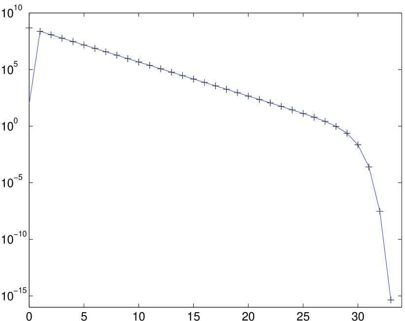
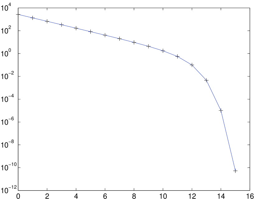
Fig. 1: $\|I-X_{k}\|$ (solid) and $\sigma(\omega^{(k)}(t_{0}))$ (pluses) for the Moler matrix (left) and the Fielder matrix (right).

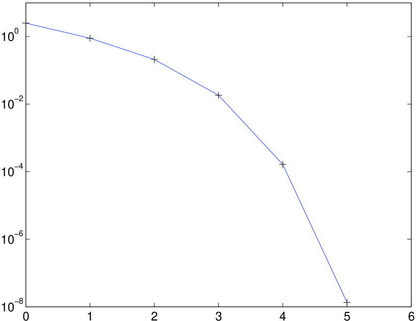
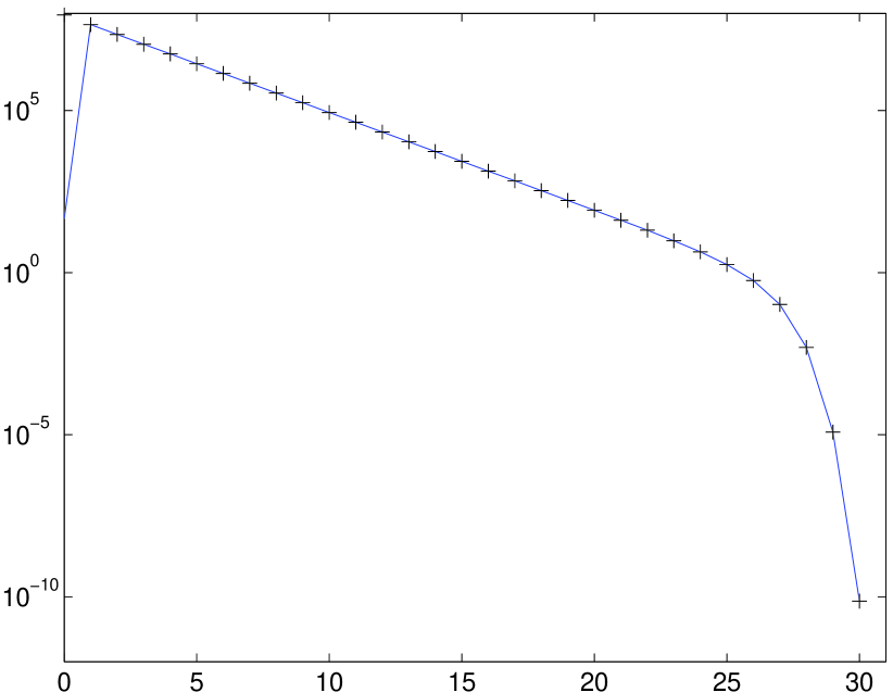
Fig. 2: $\|I-X_{k}\|$ (solid) and $\sigma(\omega^{(k)}(t_{0}))$ (pluses) for the Jordan blocks matrix (left) and the Frank matrix (right).

In the examples we observe the typical behavior of Newton’s method: An initial phase of linear convergence being followed by a phase of quadratic convergence in which the error is reduced very quickly. While the convergence bound (14) is an equality for all $k\geq 1$, it may happen that $\|I-X_{0}\|\ll\sigma(t_{0})$ as well as $\|I-X_{0}\|\ll\|I-X_{1}\|$; see the results for the Moler matrix and the Frank matrix. As shown in Theorem 2, the error is guaranteed to decrease strictly monotonically after the first step. In practice the iteration can be scaled for stability as well as for accelerating the convergence; see [1, 3] or [5, Section 8.6] for details. We give some brief comments on scaled iterations in Section 5.

4 Application to the Newton iteration for the matrix square root

Let $A\in{\mathbb{C}}^{n\times n}$ be a given, possibly singular, matrix. Any matrix $X\in{\mathbb{C}}^{n\times n}$ that satisfies $X^{2}=A$ is called a square root of $A$. For the theory of matrix square roots and many algorithms for computing them we refer to [5, Chapter 6].

One of the algorithms for computing matrix square roots is Newton’s iteration; cf. [5, Equation (6.12)]:

$$X_{0} A$$ is invertible and commutes with . (15)

$$X_{k+1}=\frac{1}{2}(X_{k}+X_{k}^{-1}A),\quad k=0,1,2,\dots\,.$$ (16)

Similar to the Newton iteration for the matrix polar decomposition, the iteration (15)–(16) can be derived by applying Newton’s method to a matrix equation, here $X^{2}-A=0$; see [5, pp. 139–140] for details. As shown in [5, Theorem 6.9], the iterates $X_{k}$ converge (under some natural assumptions) to the principal square root $A^{1/2}$, and they satisfy the convergence bound

$$\|A^{1/2}-X_{k+1}\|\leq\frac{1}{2}\,\|X_{k}^{-1}\|\,\|A^{1/2}-X_{k}\|^{2},$$

where $\|\cdot\|$ denotes any submultiplicative matrix norm. This is a bound of the classical form (4) that shows quadratic convergence.

4.1 A convergence theorem for the iteration (15)–(16)

The approach for analyzing the iteration (15)–(16) using Theorem 2 contains some differences in comparison with the one for the matrix polar decomposition. These differences will be pointed out in the derivation. Ultimately they will lead to a convergence result giving formally the same bound as in Theorem 4 (with the appropriate modifications), but containing a strong assumption on the initial matrix $X_{0}$.

As in Section 3 we consider $E={\mathbb{C}}^{n\times n}$ and the spectral norm $\|\cdot\|$. Now the mapping $G\,:\,D(G)\rightarrow E$ is defined by

$$G(X)\equiv\frac{1}{2}(X+X^{-1}A);\quad\mbox{cf. (\ref{eqn:newton2}).}$$

We need to determine $D(G)$ and define the sets $Z(t)\subseteq D(G)$ for some interval $T=(0,\tau)$, where we will again specify $\tau=\infty$ in the end.

Clearly, $D(G)$ is equal to the set of the invertible matrices in ${\mathbb{C}}^{n\times n}$, so that each $X\in Z(t)$ must be invertible. The first major difference in comparison to the iteration for the polar decomposition, where the iterates converge to a unitary matrix, is that in case of (15)–(16) the conditioning of the iterates may deteriorate during the process. In fact, when $A$ is (close to) singular, any of its square roots will be (close to) singular as well. As originally suggested by Pták in [11, 12] (also cf. [9, pp. 20–22]), such deterioration may be dealt with by requiring that each $X\in Z(t)$ satisfies

$$\sigma_{\min}(X)\geq h(t),$$

where $h$ is some positive function on $T$ that will be specified below. Further requirements for each $X\in Z(t)$ are that $X$ commutes with $A$ (cf. (15)) and that $\|X-G(X)\|\leq t$, which is the first condition in (ii) of Theorem 2. We thus define for the given matrix $A\in{\mathbb{C}}^{n\times n}$ and $t\in T=(0,\tau)$ the set

$$Z(t)\equiv\left\{X\in{\mathbb{C}}^{n\times n}\,|\,AX=XA,\;\;\sigma_{\min}(X)\geq h(t),\;\;\|X-G(X)\|\leq t\right\}\;\subset\;D(G).$$

Satisfying (i) and the second condition in (ii) of Theorem 2 will now prove the convergence of Newton’s method (15)–(16) to a matrix $X_{*}\in Z(0)$ with the error norm in each step of the iteration bounded as in (2.c) of Theorem 2. We will have a closer look at the set $Z(0)$ below.

For the second condition in (ii), let $t\in T$ and $X\in Z(t)$ be given. Since $X$ commutes with $A$, we see that the matrix $\widehat{X}\equiv G(X)$ commutes with $A$. We need to show that

$$\sigma_{\min}(\widehat{X})\geq h(\omega(t))\quad\mbox{and}\quad\|X-\widehat{X}\|\leq\omega(t)$$

for a positive function $h$ on $T$ and a rate of convergence $\omega$ on $T$. Using $\|X-\widehat{X}\|\leq t$ and $\sigma_{\min}(X)\geq h(t)$, we get

$$\sigma_{\min}(\widehat{X}) = \sigma_{\min}(X-(X-\widehat{X}))\geq\sigma_{\min}(X)-\|X-\widehat{X}\|\geq h(t)-t,$$

from which we obtain the condition

$$h(t)-t\geq h(\omega(t)).$$ (17)

Next, note that $\widehat{X}=G(X)$ can equivalently be written as $X^{2}-2X\widehat{X}+A=0.$ Using this and the fact that $X$ and $\widehat{X}$ commute, we get

$$\widehat{X}^{2}-A=\widehat{X}^{2}-A+(X^{2}-2X\widehat{X}+A)=(X-\widehat{X})^{2}.$$ (18)

Consequently,

$$\|\widehat{X}-G(\widehat{X})\| = \frac{1}{2}\|\widehat{X}^{-1}(A-\widehat{X}^{2})\|\leq\frac{1}{2}\|\widehat{X}^{-1}\|\,\|\widehat{X}^{2}-A\|=\frac{1}{2}\frac{\|(X-\widehat{X})^{2}\|}{\sigma_{\min}(\widehat{X})}$$

$$\leq \frac{1}{2}\frac{t^{2}}{h(t)-t},$$

which gives the condition

$$\frac{1}{2}\frac{t^{2}}{h(t)-t}\leq\omega(t).$$ (20)

The inequality in (4.1) represents the second major difference in the derivation compared to the matrix polar decomposition. In (4.1) we have used the submultiplicativity of the matrix norm, while in (8)–(10) no inequalities occur because the matrices are effectively diagonal when considered under the unitarily invariant norm. The absence of inequalities in the derivation ultimately led to a convergence bound in Theorem 4 that is attained in every step $k\geq 1$.

The two (sufficient) conditions (17) and (20) for $\widehat{X}\in Z(\omega(t))$ form a system of functional inequalities that was ingeniously solved by Pták in [11]. Here it suffices to say that for any $\gamma\geq 0$ the rate of convergence $\omega$ on $T\equiv(0,\infty)$ and the corresponding function $\sigma$ given by

$$\omega(t)\equiv\frac{1}{2}\,\frac{t^{2}}{(t^{2}+\gamma^{2})^{1/2}}\quad\mbox{and}\quad\sigma(t)\equiv t-\gamma+(t^{2}+\gamma^{2})^{1/2}$$ (21)

(i.e. (12) and (13) for $\gamma=1$) and the function

$$h(t)\equiv\gamma+\sigma(t),$$

which is positive on $T=(0,\infty)$, satisfy the conditions (17) and (20).

It remains to satisfy the condition (i) in Theorem 2, i.e., to show that for some $t_{0}>0$ there exists an $X_{0}\in Z(t_{0})$. This will determine the parameter $\gamma\geq 0$, which so far is not specified. We require that $X_{0}$ commutes with $A$, and that

$$\sigma_{\min}(X_{0})\geq h(t_{0})=t_{0}+(t_{0}^{2}+\gamma^{2})^{1/2}\quad\mbox{and}\quad\frac{1}{2}\|X_{0}^{-1}A-X_{0}\|\leq t_{0}.$$

If we define

$$t_{0}\equiv\frac{1}{2}\|X_{0}^{-1}A-X_{0}\|,$$

then the second inequality is automatically satisfied. Some simplifications of the first inequality lead to

$$\sigma_{\min}(X_{0})\,(\sigma_{\min}(X_{0})-2t_{0})\geq\gamma^{2}.$$

Hence we must have $\sigma_{\min}(X_{0})-2t_{0}\geq 0$, and

$$\gamma=\gamma_{0}\equiv\sigma_{\min}^{1/2}(X_{0})(\sigma_{\min}(X_{0})-2t_{0})^{1/2}$$ (22)

is a feasible choice of the parameter in order to satisfy all conditions. Theorem 2 now shows that under these conditions the iterative algorithm (15)–(16) is meaningful and converges to some $X_{*}\in Z(0)\subseteq\overline{D(G)}$.

Let us now consider the set $Z(0)$. First note that, for any $t>0$ and $X\in Z(t)$,

$$\|\widehat{X}^{2}-A\|\leq\|X-\widehat{X}\|^{2}\leq t^{2};$$

see (18). Taking the limit $t\rightarrow 0$ we see that each $X\in Z(0)$ must satisfy $X^{2}=A$. Moreover, each $X\in Z(0)$ commutes with $A$ and satisfies $\sigma_{\min}(X)\geq h(0)=\gamma_{0}$. If $\gamma_{0}>0$, then all matrices in the limiting set $Z(0)$ are invertible and $Z(0)\subset D(G)$. If $\gamma_{0}=0$, then a singular limiting matrix is possible and in this case $Z(0)$ is not a subset of $D(G)$. This will be discussed further below and numerically illustrated in the next section.

In summary, we have shown the following result.

Theorem 5.

Let $A\in{\mathbb{C}}^{n\times n}$ and let $X_{0}\in{\mathbb{C}}^{n\times n}$ be invertible and commute with $A$. If

$$\sigma_{\min}(X_{0})\geq\|X_{0}^{-1}A-X_{0}\|\equiv 2t_{0},$$ (23)

then the iterative algorithm (15)–(16) is meaningful and its sequence of iterates $\{X_{k}\}$ converges to a matrix $X_{*}\in{\mathbb{C}}^{n\times n}$ that commutes with $A$ and satisfies $X_{*}^{2}=A$. Moreover, with $\omega$ and $\sigma$ as in (21), where $\gamma=\gamma_{0}$ as in (22), we have

$$\|X_{*}-X_{k}\|\leq\sigma(\omega^{(k)}(t_{0})),\quad k=0,1,2,\dots\,.$$ (24)

If $\gamma_{0}>0$, then $X_{*}$ is invertible with $\sigma_{\min}(X_{*})\geq\gamma_{0}$.

We will now discuss the condition (23). First note that from

$$\|X_{0}^{-1}A-X_{0}\|\leq\|X_{0}^{-1}\|\,\|A-X_{0}^{2}\|=\sigma_{\min}^{-1}(X_{0})\,\|A-X_{0}^{2}\|$$

it follows that (23) is implied by $\sigma_{\min}^{2}(X_{0})\geq\|A-X_{0}^{2}\|$. It therefore appears that the condition is satisfied whenever $X_{0}$ commutes with $A$, is well conditioned and sufficiently close (in norm) to a square root of $A$. However, as we will see below, the condition (23) seriously limits the applicability of Theorem 5.

The fact that the initial matrix $X_{0}$ has to satisfy some conditions (unlike in the case of Theorem 4) is to be expected, since not every matrix $A$ has a square root; cf. [5, Section 1.5]. If an invertible matrix $X_{0}$ that commutes with $A$ and satisfies (23) can be found, then the convergence of the Newton iteration guarantees the existence of a square root of $A$. Pták referred to this as an iterative existence proof [12].

Now let $A\neq 0$ be real and symmetric with the real eigenvalues $\lambda_{1}\leq\cdots\leq\lambda_{n}$ and let $X_{0}=\alpha I$ for some real $\alpha\neq 0$. Then $X_{0}$ is invertible and commutes with $A$, and (23) becomes

$$\alpha^{2}\geq\|A-\alpha^{2}I\|=\max_{1\leq j\leq n}\,|\lambda_{j}-\alpha^{2}|=\max\,\{\,|\lambda_{1}-\alpha^{2}|,\,|\lambda_{n}-\alpha^{2}|\,\}.$$ (25)

This condition cannot be satisfied if $\lambda_{1}<0$. (Note that in this case the principal square root of $A$ does not exist [5, Theorem 1.29].) On the other hand, if $\lambda_{1}\geq 0$ and hence $A$ is positive semidefinite, then a simple computation shows that each matrix of the form

$$X_{0}=\alpha I\quad\mbox{with}\quad|\alpha|\geq\left(\frac{\lambda_{1}+\lambda_{n}}{2}\right)^{1/2}>0$$ (26)

satisfies (23) and thus the conditions of Theorem 5. If $\lambda_{1}=0$ and hence $A$ is singular, then for every $|\alpha|\geq(\lambda_{n}/2)^{1/2}$ equality holds in (25). We then get $\gamma_{0}=0$ in (22), and in this case the rate of convergence is

$$\omega(t)=\frac{t}{2},\quad\mbox{giving}\quad\omega^{(k)}(t)=\frac{t}{2^{k}}\quad\mbox{and}\quad\sigma(\omega^{(k)}(t))=\frac{t}{2^{k-1}}.$$ (27)

A numerical example with a real, symmetric and singular matrix is shown in the right part of Figure 3.

The following result shows that, despite the inequality in (4.1), the bound (24) is attained in every step for certain $A$ and $X_{0}$.

Corollary 6.

If $A\in{\mathbb{R}}^{n\times n}$ is symmetric with eigenvalues $0\leq\lambda_{1}\leq\cdots\leq\lambda_{n}$ and $X_{0}$ is as in (26), then the conditions of Theorem 5 are satisfied, the sequence of iterates $\{X_{k}\}$ of (15)–(16) converges to the principal square root $A^{1/2}$ of $A$, and the bound (24) is an equality in each step $k\geq 0$.

Proof.

We already know that $A$ and $X_{0}$ satisfy the conditions of Theorem 5. Let $A=Q\Lambda Q^{T}$ be an eigendecomposition of $A$ with $Q\in{\mathbb{R}}^{n\times n}$ orthogonal and $\Lambda={\rm diag}(\lambda_{1},\dots,\lambda_{n})$. Then $A^{1/2}=Q\Lambda^{1/2}Q^{T}$ with $\Lambda^{1/2}={\rm diag}(\lambda_{1}^{1/2},\dots,\lambda_{n}^{1/2})$ is the principal square root of $A$. It suffices to show that $\|A^{1/2}-X_{0}\|=\sigma(t_{0})$, then the result follows from the last part of Theorem 2.

Using $X_{0}=\alpha I$ and $|\alpha|\geq\left(\frac{\lambda_{1}+\lambda_{n}}{2}\right)^{1/2}>0$ we get

$$t_{0} = \frac{1}{2}\|\alpha^{-1}\Lambda-\alpha I\|=\frac{1}{2|\alpha|}\max_{1\leq j\leq n}\,|\lambda_{j}-\alpha^{2}|=\frac{\alpha^{2}-\lambda_{1}}{2|\alpha|},$$

$$\gamma_{0} = \sigma_{\min}(X_{0})^{1/2}\,(\sigma_{\min}(X_{0})-2t_{0})^{1/2}=(\alpha^{2}-2|\alpha|t_{0})^{1/2}=\lambda_{1}^{1/2},$$

and thus

$$\sigma(t_{0}) = t_{0}-\gamma_{0}+(t_{0}^{2}+\gamma_{0}^{2})^{1/2}=t_{0}-\gamma_{0}+(t_{0}^{2}+\alpha^{2}-2|\alpha|t_{0})^{1/2}=t_{0}-\gamma_{0}+(|\alpha|-t_{0})$$

$$= |\alpha|-\gamma_{0}=|\alpha|-\lambda_{1}^{1/2}=\max_{1\leq j\leq n}\,|\,|\alpha|-\lambda_{j}^{1/2}\,|=\|A^{1/2}-X_{0}\|,$$

where we have used that $|\alpha|\geq t_{0}$ and $|\alpha|\geq\left(\frac{\lambda_{1}+\lambda_{n}}{2}\right)^{1/2}>\frac{\lambda_{1}^{1/2}+\lambda_{n}^{1/2}}{2}$. ∎

Similar to Theorem 4, the sharpness result in the above corollary could also be derived using results of Potra and Pták (e.g., [9, Proposition 5.10]), when one interprets the iteration (15)–(16) for a real and symmetric positive semidefinite matrix $A$ and with $X_{0}=\alpha I$ in terms of $n$ uncoupled scalar iterations.

Finally, we note that for a real and symmetric positive definite matrix $A$ with eigenvalues $0<\lambda_{1}\leq\cdots\leq\lambda_{n}$ the condition (23) with $X_{0}=\alpha A$ and a real $\alpha\neq 0$ becomes

$$\lambda_{1}\geq\max_{1\leq j\leq n}\,|\lambda_{j}-\alpha^{-2}|=\max\,\{\,|\lambda_{1}-\alpha^{-2}|,\,|\lambda_{n}-\alpha^{-2}|\,\}.$$

An elementary computation shows that this condition cannot be satisfied for any real $\alpha\neq 0$ when $\lambda_{n}/\lambda_{1}>3$. If $1<\lambda_{n}/\lambda_{1}\leq 3$, then $\lambda_{n}=\mu\lambda_{1}$ for some $1<\mu\leq 3$, and $\alpha=(\delta\lambda_{1})^{-1/2}$ with $\mu-1\leq\delta\leq 2$ is a feasible choice. Obviously, the conditions on $A$ and $\alpha$ for the applicability of Theorem 5 are in this case much more restrictive than for initial matrices of the form $X_{0}=\alpha I$.

4.2 Numerical examples

We will now illustrate Theorem 5 on some numerical examples. As originally shown by Higham [4], the Newton iteration for the matrix square root in the form (15)–(16) is numerically unstable; see also [5, Section 6.4]. For our numerical experiments we have used the mathematically equivalent “IN iteration” (cf. [5, Equation (6.20)]), originally derived by Iannazzo [6]:

$$X_{0} A E_{0}=\frac{1}{2}(X_{0}^{-1}A-X_{0})$$ is invertible and commutes with , and . (28)

$$X_{k+1}=X_{k}+E_{k}\quad\mbox{and}\quad E_{k+1}=-\frac{1}{2}E_{k}X_{k+1}^{-1}E_{k},\quad k=0,1,2,\dots\,.$$ (29)

This variant is numerically stable and has a limiting accuracy on the order of the unit roundoff [5, Table 6.2]. In practice one uses scalings for accelerating the convergence [5, Section 6.5]; for brief comments on scalings see Section 5.

We use three initial matrices of the form

$$X_{0}=\alpha_{j}I\quad\mbox{with}\quad\alpha_{j}=2^{j}\left(\frac{\|A\|}{2}\right)^{1/2},\quad j=1,2,3.$$

This choice of $\alpha_{j}$ is motivated by the argument leading to (26), although this argument only applies to real symmetric matrices. We point out that for none of our example matrices $A$ an initial matrix of the form $X_{0}=\alpha_{j}A$ satisfies the condition (23), although the Newton method always converges when started with them (except for the singular matrix defined below, where $X_{0}=\alpha_{j}A$ cannot be used). This demonstrates the severe restriction of the condition (23) for the general applicability of Theorem 5.

For the given $X_{0}$ we first run the iteration (28)–(29) until it converges to a matrix $X_{*}$ that is an approximate square root of $A$. Typically in our examples $\|A-X_{*}^{2}\|\approx 10^{-14}$. We then run the iteration again and compute the error $\|X_{*}-X_{k}\|$ in each step $k\geq 0$. These errors are shown by the solid lines in Figures 3–5. The corresponding a priori values $\sigma(\omega^{(k)}(t_{0}))$ of the upper bound (24) are shown by the pluses $(+)$ in Figures 3–4.

We present numerical results for the Moler matrix (left part of Figure 3), the Jordan blocks matrix (left part of Figure 4) and the Frank matrix (Figure 5) as defined in Section 3.2. We do not use the symmetric indefinite Fiedler matrix from Section 3.2 since the Newton iteration (15)–(16) for this matrix does not converge when started with $X_{0}=\alpha_{j}I$. Instead, we present results for the following matrices:

Singular matrix. The $40\times 40$ diagonal matrix with eigenvalues $0,1,\dots,39$. The results for this matrix are shown in the right part of Figure 3.

Modified Jordan blocks matrix. The $100\times 100$ matrix ${\rm diag}(J_{50}(1.0),J_{50}(2.5))$, i.e., the previous Jordan blocks matrix with the eigenvalue 1.5 replaced by 1.0. The results for this matrix are shown in the right part of Figure 4.

For the Moler matrix and the singular matrix we have $\alpha_{j}\geq\left(\frac{\lambda_{1}+\lambda_{n}}{2}\right)^{1/2}$ for $j=1,2,3$. Hence the bound (24) is sharp by Corollary 6, which is illustrated by the numerical results. While for the Moler matrix we observe the typical behavior of Newton’s method, the convergence for the singular matrix is linear throughout, which is explained by (27). The bound (24) is very tight for the Jordan blocks matrix, but for the modified Jordan blocks matrix the actual convergence acceleration in the quadratic phase is larger than the one predicted by the bound.

Finally, for the Frank matrix none of the initial matrices $X_{0}=\alpha_{j}I$ with $\alpha_{j}=2^{j}\left(\|A\|/2\right)^{1/2}$ (here $\|A\|\approx 79.7$) satisfies the condition (23), and hence no convergence bound is given by Theorem 5. The constants in condition (23) have the following values:

$j$	$\sigma_{\min}(X_{0})$	$2t_{0}=\|X_{0}^{-1}A-X_{0}\|$
1	9.7710	10.1148
2	19.5420	19.7128
3	39.0839	39.1692

Although Theorem 5 is not applicable, the Newton iteration (eventually) converges, as shown in Figure 5. The figure also shows that the convergence is characterized by an initial phase of complete stagnation. It is a challenging task to determine a rate of convergence that can closely describe such behavior.

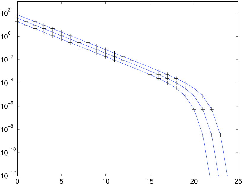
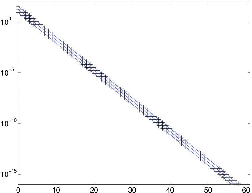
Fig. 3: $\|X_{*}-X_{k}\|$ (solid) and $\sigma(\omega^{(k)}(t_{0}))$ (pluses) for the Moler matrix (left) and the singular matrix (right).

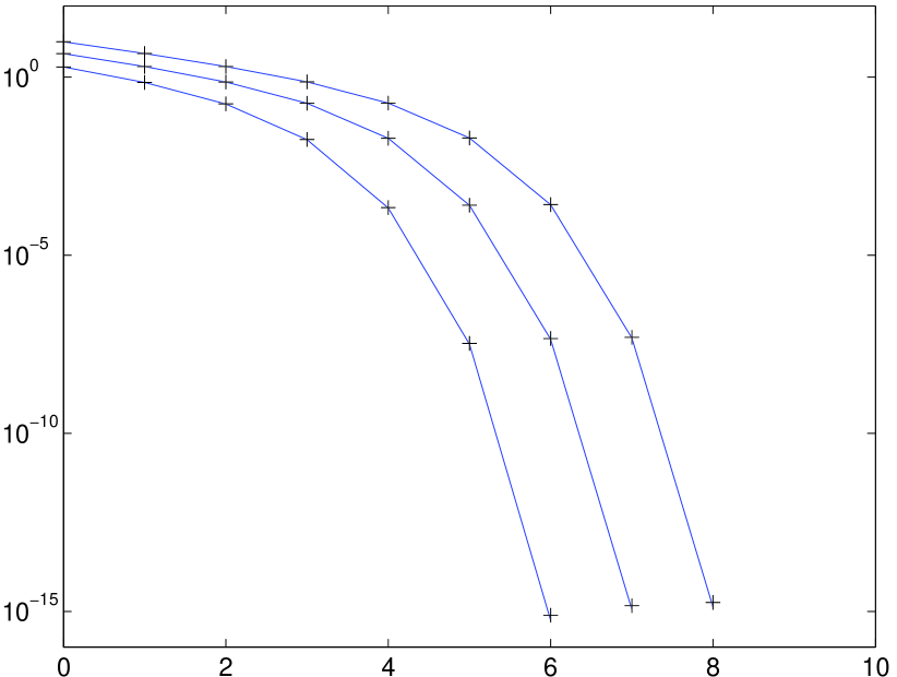
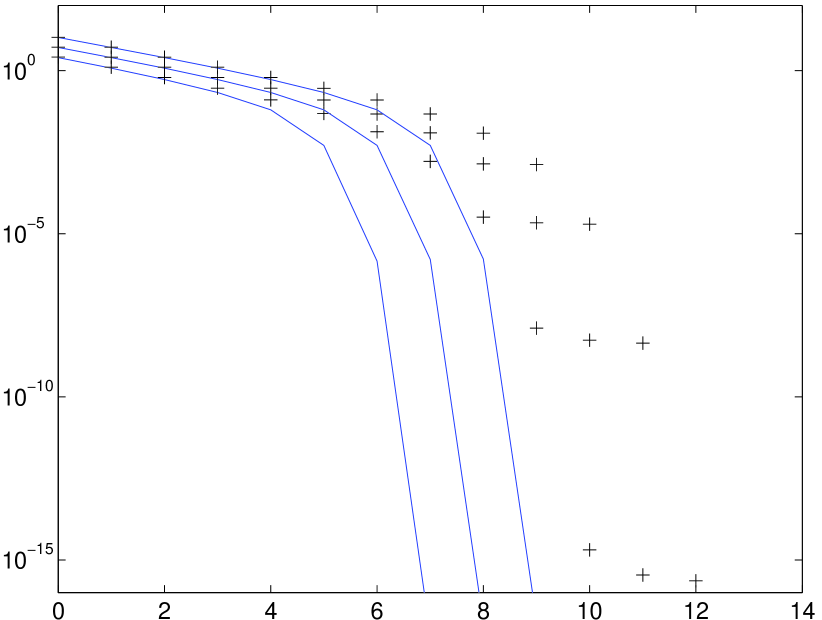
Fig. 4: $\|X_{*}-X_{k}\|$ (solid) and $\sigma(\omega^{(k)}(t_{0}))$ (pluses) for the Jordan blocks matrix (left) and the modified Jordan blocks matrix (right).

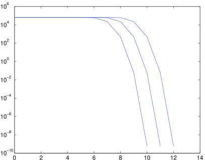
Fig. 5: $\|X_{*}-X_{k}\|$ (solid) for the Frank matrix.

5 Discussion and outlook

The main purpose of Pták’s method of nondiscrete induction is to derive error bounds for iterative processes that can be tight throughout the iteration. As demonstrated for the Newton iteration for the matrix polar decomposition and the matrix square root, the approach can indeed give very tight, even sharp bounds in practical applications. However, we have also seen that the approach has some limitations, in particular for (highly) nonnormal matrices. The results for the matrix square root iteration applied to the Frank matrix illustrate an observation we made: For a general nonnormal matrix it appears to be very difficult to determine (easily and a priori) an initial matrix $X_{0}$ that satisfies the assumptions of Theorem 5. The derivation of strategies for computing such $X_{0}$ is beyond the scope of this paper. We also did not analyze more closely the observations about the tightness of the bound (24) for the two Jordan blocks matrices. Such investigations are subject of future work. Note that the difficulty of nonormality does not appear in case of the Newton iteration for the matrix polar decomposition, since it effectively acts on diagonal matrices.

Convergence of an iteration means that a solution of a certain equation exists. In case of the Newton iteration for the matrix square root this equation is $X^{2}-A=0$ for the given (square) matrix $A$. Finding an initial matrix $X_{0}$ that satisfies the assumptions of Theorem 5 guarantees that the matrix $A$ has a square root (“iterative existence proof”). The fact that existence and convergence are studied and proven simultaneously may be one reason why the (sufficient) conditions in Theorem 5 are more restrictive than other types of conditions for convergence of the iteration under the assumption that a square root exists. From a practical point of view it would be of interest to obtain variants of Theorem 5 with weaker conditions on $X_{0}$.

As described in Section 2, an essential constructive idea in the method of nondiscrete induction is the comparison of consecutive iterates. The method therefore is suited best for iterations where a new iterate is generated using information only from the previous step, and Newton-type methods are ideal examples in this respect. Methods that generate new iterates based on information from several or all previous steps possibly can be analyzed using the concept of multidimensional rates of convergence described in [9, Chapter 3]. It also would be interesting to appropriately generalize the theory of Potra and Pták to scaled or, more generally, parameter-dependent iterations. As briefly mentioned in Sections 3.2 and 4.2, scalings are used in practice for numerical stability properties or for accelerating Newton-type matrix iterations. Including parameters that are not known a priori within the method of nondiscrete induction is an interesting subject of further work. In the framework established by Theorem 2 it may be possible to include parameters depending only on the latest iterate $x_{k}$ by appropriately defining the sets $Z(t)$. More sophisticated parameter-dependence requires extensions of Theorem 2. Such extensions may also lead to new convergence results for nonlinear iterative schemes like Krylov subspace methods (see, e.g., [7]), where new iterates are generated using information from all previous steps and parameters that are not known a priori.

Acknowledgments. Many thanks to Nick Higham, Gérard Meurant, Zdeněk Strakoš and Petr Tichý for helpful comments.

References

- [1] R. Byers and H. Xu, A new scaling for Newton’s iteration for the polar decomposition and its backward stability, SIAM J. Matrix Anal. Appl., 30 (2008), pp. 822–843.
- [2] P. Deuflhard, Newton Methods for Nonlinear Problems. Affine Invariance and Adaptive Algorithms, vol. 35 of Springer Series in Computational Mathematics, Springer, Heidelberg, 2011. First softcover printing of the 2006 corrected printing.
- [3] N. J. Higham, Computing the polar decomposition—with applications, SIAM J. Sci. Statist. Comput., 7 (1986), pp. 1160–1174.
- [4] , Newton’s method for the matrix square root, Math. Comp., 46 (1986), pp. 537–549.
- [5] , Functions of Matrices. Theory and Computation, Society for Industrial and Applied Mathematics (SIAM), Philadelphia, PA, 2008.
- [6] B. Iannazzo, A note on computing the matrix square root, Calcolo, 40 (2003), pp. 273–283.
- [7] J. Liesen and Z. Strakoš, Krylov Subspace Methods. Principles and Analysis, Numerical Mathematics and Scientific Computation, Oxford University Press, Oxford, 2013.
- [8] F.-A. Potra and V. Pták, Sharp error bounds for Newton’s process, Numer. Math., 34 (1980), pp. 63–72.
- [9] F. A. Potra and V. Pták, Nondiscrete Induction and Iterative Processes, vol. 103 of Research Notes in Mathematics, Pitman (Advanced Publishing Program), Boston, MA, 1984.
- [10] V. Pták, Some metric aspects of the open mapping and closed graph theorems, Math. Ann., 163 (1966), pp. 95–104.
- [11] , The rate of convergence of Newton’s process, Numer. Math., 25 (1975/76), pp. 279–285.
- [12] , Nondiscrete mathematical induction and iterative existence proofs, Linear Algebra and Appl., 13 (1976), pp. 223–238.
- [13] , What should be a rate of convergence?, RAIRO Anal. Numér., 11 (1977), pp. 279–286.
- [14] , Iterative processes, functional inequations and the Newton method, Exposition. Math., 7 (1989), pp. 49–68.