An optimal survey geometry of weak lensing survey: minimizing super-sample covariance

Abstract

Upcoming wide-area weak lensing surveys are expensive both in time and cost and require an optimal survey design in order to attain maximum scientific returns from a fixed amount of available telescope time. The super-sample covariance (SSC), which arises from unobservable modes that are larger than the survey size, significantly degrades the statistical precision of weak lensing power spectrum measurement even for a wide-area survey. Using the 1000 mock realizations of the log-normal model, which approximates the weak lensing field for a $\Lambda$-dominated cold dark matter model, we study an optimal survey geometry to minimize the impact of SSC contamination. For a continuous survey geometry with a fixed survey area, a more elongated geometry such as a rectangular shape of 1:400 side-length ratio reduces the SSC effect and allows for a factor 2 improvement in the cumulative signal-to-noise ratio ($S/N$) of power spectrum measurement up to $\ell_{\rm max}\simeq$ a few $10^{3}$, compared to compact geometries such as squares or circles. When we allow the survey geometry to be disconnected but with a fixed total area, assuming $1\times 1$ sq. degrees patches as the fundamental building blocks of survey footprints, the best strategy is to locate the patches with $\sim 15$ degrees separation. This separation angle corresponds to the scale at which the two-point correlation function has a negative minimum. The best configuration allows for a factor 100 gain in the effective area coverage as well as a factor 2.5 improvement in the $S/N$ at high multipoles, yielding a much wider coverage of multipoles than in the compact geometry.

1 Introduction

Weak gravitational lensing of foreground large-scale structure induces a coherent, correlated distortion in distant galaxy images, the so-called cosmic shear  (e.g., Bartelmann & Schneider 2001; Hoekstra & Jain 2008; Munshi et al. 2008). The cosmic shear signal is statistically measurable, e.g., by measuring the angular two-point correlation function of galaxy images. The current state-of-art measurements are from the Canada-France Hawaii Telescope Lensing Survey (CFHTLenS; Kilbinger et al. 2013; Heymans et al. 2013) and the Sloan Digital Sky Survey (SDSS; Huff et al. 2014; Lin et al. 2012; Mandelbaum et al. 2013), which were used to constrain cosmological parameters such as the present-day amplitude of density fluctuation $\sigma_{8}$ and the matter density parameter $\Omega_{\rm m}$. There are various on-going and planned surveys aimed at achieving the high precision measurement such as the Subaru Hyper Suprime-Cam (HSC; Miyazaki, et al. 2006), the Kilo Degree Survey (KiDS), the Dark Energy Survey (DES), the Panoramic Survey Telescope and Rapid Response System (Pan-STARRS), and then ultimately the Large Synoptic Survey Telescope (LSST), the Euclid and the WFIRST (Spergel et al. 2013).

Upcoming wide-area galaxy surveys are expensive both in time and cost. To attain the full potential of the galaxy surveys for a limited amount of available telescope time, it is important to explore an optimal survey design. The statistical precision of the cosmic shear two-point correlation function or the Fourier-transformed counterpart, the power spectrum, is determined by their covariance matrix that itself contains two contributions; the shape noise and the sample variance caused by an incomplete sampling of the fluctuations due to a finite-area survey.

Even though the initial density field is nearly Gaussian, the sample variance of large-scale structure probes (here cosmic shear) gets substantial non-Gaussian contributions from the nonlinear evolution of large-scale structure (Meiksin & White 1999; Scoccimarro et al. 1999; Hu & White 2001; Cooray & Hu 2001). Most of the useful information in the cosmic shear signal lies in the deeply nonlinear regime (Jain & Seljak 1997; Bernardeau et al. 1997). The super-sample covariance (SSC) is the sampling variance caused by coupling of short-wavelength modes relevant for the power spectrum measurement with very long-wavelength modes larger than the survey size (Takada & Hu 2013). It has been shown to be the largest non-Gaussian contribution to the power spectrum covariance over a wide range of modes from the weakly to deeply nonlinear regime (Neyrinck et al. 2006; Neyrinck & Szapudi 2007; Lee & Pen 2008; Takada & Jain 2009; Takahashi et al. 2009; Sato et al. 2009; Takahashi et al. 2011b; de Putter et al. 2012; Kayo et al. 2013; Takada & Spergel 2013; Li et al. 2014a, b) (see also Hu & Kravtsov 2003; Rimes & Hamilton 2005; Hamilton et al. 2006, for the pioneering work). The SSC depends on a survey geometry through the variance of average convergence mode within the survey window, $(\sigma_{W})^{2}\equiv\left\langle\bar{\kappa}_{W}^{2}\right\rangle$ (here $\bar{\kappa}_{W}$ is the mean convergence averaged within the survey area), which differs from the dependence of other covariance terms that scale as $1/\Omega_{S}$ ($\Omega_{S}$ is the survey area).

The purpose of this paper is to study an optimal survey strategy for the lensing power spectrum measurement taking account of the SSC contamination. We study both cases of continuous geometry and sparse sampling strategy. Although previous works showed that the sparse sampling helps to reduce the sample variance and to give an access to larger-angle scales than in a continuous geometry (Kaiser 1986, 1998; Kilbinger & Schneider 2004) (also see Blake et al. 2006; Paykari & Jaffe 2013; Chiang et al. 2013, for the similar discussion on the galaxy clustering analysis), we here pay particular attention to optimization of survey geometry to minimize the SSC contamination. To study these issues, we use realizations of weak lensing convergence field constructed based on the log-normal model, which approximately describes the weak lensing field for a $\Lambda$CDM model (also see Chiang et al. 2013, for the similar study along the galaxy redshift survey). For the log-normal model we can analytically derive the power spectrum covariance following the formulation in Takada & Hu (2013), and use the analytical model to justify the results of the log-normal simulations.

The structure of this paper is as follows. In Section 2 we briefly review the log-normal model, and then describe the log-normal simulations and the analytical models. In Section 3 we show the main results of this paper, and then study the sparse sampling strategy in Section 4. Section 5 is devoted to conclusion and discussion. Throughout this paper we adopt the concordance $\Lambda$CDM model, which is consistent with the WMAP 7-year results (Komatsu et al. 2011). The model is characterized by the matter density $\Omega_{\rm m}=0.272$, the baryon density $\Omega_{\rm b}=0.046$, the cosmological constant density $\Omega_{\Lambda}=0.728$, the spectral index of the primordial power spectrum $n_{\rm s}=0.97$, the present-day rms mass density fluctuations $\sigma_{8}=0.81$, and the Hubble expansion rate today $H_{0}=70.0~{}$km s^-1 Mpc^-1.

2 Method

2.1 Log-normal convergence field

To approximate the weak lensing convergence field for a $\Lambda$CDM model, we employ the log-normal model. The previous works based on ray-tracing simulations (see Taruya et al. 2002; Das & Ostriker 2006; Hilbert et al. 2007; Takahashi et al. 2011a; Neyrinck et al. 2009; Joachimi et al. 2011; Seo et al. 2012) have shown that the log-normal model can serve as a fairly good approximation of the lensing field, originating from the fact that the three-dimensional matter field in large-scale structure is also approximated by the log-normal distribution (e.g. Coles & Jones 1991; Kofman et al. 1994; Kayo et al. 2001). The main reason of our use of the log-normal model is twofold; it allows us to simulate many realizations of the lensing field without running ray-tracing simulations as well as allows us to analytically compute statistical properties of the lensing field including the non-Gaussian features.

We assume that the lensing convergence field, $\kappa({\boldsymbol{\theta}})$, obeys the following one-point probability distribution function:

$$P(\kappa) = \frac{1}{\sqrt{2\pi}(\kappa/|\kappa_{0}|+1)\sigma_{\rm G}}$$ (1)

$$\times\exp\left[-\dfrac{\left\{|\kappa_{0}|\ln\left(\kappa/|\kappa_{0}|+1\right)+\sigma_{\rm G}^{2}/(2|\kappa_{0}|)\right\}^{2}}{2\sigma_{\rm G}^{2}}\right],$$

for $\kappa>-|\kappa_{0}|$, and we set $P(\kappa)=0$ for $\kappa\leq-|\kappa_{0}|$. Note that the above distribution satisfies $\int_{-|\kappa_{0}|}^{\infty}\!d\kappa~{}P(\kappa)=1$ as well as $\int_{-|\kappa_{0}|}^{\infty}\!d\kappa~{}\kappa P(\kappa)=0$. The variance is $\sigma_{\kappa}^{2}=\int_{-|\kappa_{0}|}^{\infty}\!d\kappa~{}\kappa^{2}P(\kappa)=|\kappa_{0}|^{2}[\exp(\sigma_{\rm G}^{2}/|\kappa_{0}|^{2})-1]$. The log-normal distribution is specified by two parameters, $\sigma_{\rm G}$ and $\kappa_{0}$. Throughout this paper, as for $\kappa_{0}$, we use the empty beam value for the fiducial cosmological model and the assumed source redshift (Jain et al. 2000); $\kappa_{0}=-0.050$ for source redshift $z_{s}=0.9$.

Statistical properties of the log-normal convergence field are fully characterized by the two-point correlation function of $\kappa({\boldsymbol{\theta}})$ (see below). What we meant by “fully” is any higher-order functions of the log-normal field are given as a function of products of the two-point function, but in a different form those of a Gaussian field. As for the convergence power spectrum, we employ the model that well reproduces the power spectrum seen in ray-tracing simulations of a $\Lambda$CDM model (e.g., Bartelmann & Schneider 2001):

$$C(\ell)=\frac{9H_{0}^{4}\Omega_{\rm m}^{2}}{4c^{4}}\int_{0}^{r_{\rm s}}\!\!\mathrm{d}r\frac{\left(r_{\rm s}-r\right)^{2}}{a(r)^{2}r_{\rm s}^{2}}P_{\delta}\!\left(k=\frac{\ell}{r};a(r)\right),$$ (2)

where $r_{\rm s}$ is the comoving distance to the source, $a(r)$ is the scale factor at the distance $r$, and $P_{\delta}(k;a)$ is the matter power spectrum given as a function of $k$ and $a$. Note that we throughout this paper consider a single source redshift $z_{s}$ for simplicity; $z_{s}=0.9$. In order to include effects of nonlinear gravitational clustering, we use the revised version of halo-fit model (Smith et al. 2003; Takahashi et al. 2012), which can be analytically computed once the linear matter power spectrum and cosmological model are specified. We employ the fitting formula of Eisenstein & Hu (1999) to compute the input linear power spectrum.

2.2 Power spectrum and covariance estimation from the simulated log-normal lensing maps

In order to estimate an expected measurement accuracy of the lensing power spectrum against an assumed geometry of a hypothetical survey, we use $1000$ simulation maps of the log-normal homogeneous and isotropic convergence field.

Following the method in Neyrinck et al. (2009) (also see Hilbert et al. 2011), we generate the maps as follows. (i) We choose the target power spectrum, $C(\ell)$, which the simulated log-normal field is designed to obey. We employ the power spectrum $C(\ell)$ expected for the assumed $\Lambda$CDM model and source redshift $z_{s}=0.9$, computed from Eq. (2). The source redshift is chosen to mimic the mean source redshift for a Subaru Hyper Suprime-Cam type survey. For another parameter $\kappa_{0}$ needed to specify the log-normal model, we adopt the empty beam value in the cosmology, $\kappa_{0}=-0.050$. Provided the target power spectrum $C(\ell)$ and $\kappa_{0}$, we compute the power spectrum for the corresponding Gaussian field, $C_{\rm G}(\ell)$, from the mapping relation between the log-normal and Gaussian fields (see below). (ii) Using the Fast Fourier Transform (FFT) method, we generate a Gaussian homogeneous and isotropic field, $\kappa_{\rm G}({\boldsymbol{\theta}})$, from the power spectrum $C_{\rm G}(\ell)$. In making the map, we adopt $12180\times 12180$ grids for an area of $203\times 203~{}{\rm deg}^{2}$ ($\simeq 4\pi$ steradian, i.e. all-sky area) so that the grid scale is 1 arcmin on a side (because $203\times 60=12180$). Since we used the FFT method, the simulated Gaussian map obeys the periodic boundary condition; no Fourier mode beyond the map size ($203~{}$deg.) exists. The mean of $\kappa_{\rm G}$ is zero and the one-point 2nd-order moments is defined as $\sigma_{\rm G}^{2}\equiv\langle\kappa_{\rm G}({\boldsymbol{\theta}})^{2}\rangle$ (the variance of the FFT grid-based field). (iii) We add the constant value, $-\sigma_{\rm G}^{2}/(2|\kappa_{0}|)$, to each grid so that the mean of the Gaussian field becomes $\left\langle\kappa_{\rm G}({\boldsymbol{\theta}})\right\rangle=-\sigma_{\rm G}^{2}/(2|\kappa_{0}|)$. This constant shift is necessary so that the mean of the log-normal field is zero after the mapping (Eq. 3). (iv) Employing the log-normal mapping

$$\kappa({\boldsymbol{\theta}})=|\kappa_{0}|\left[\exp\left(\frac{\kappa_{\rm G}({\boldsymbol{\theta}})}{|\kappa_{0}|}\right)-1\right]$$ (3)

we evaluate the log-normal field, $\kappa({\boldsymbol{\theta}})$, at each grid in the map. The variance of the log-normal field is exactly related to that of the Gaussian field $\kappa_{\rm G}({\boldsymbol{\theta}})$ via $\sigma_{\kappa}^{2}=|\kappa_{0}|^{2}[\exp(\sigma_{\rm G}^{2}/|\kappa_{0}|^{2})-1]$. Since the grid size of 1 arcmin is still in the weak lensing regime, $\sigma_{\kappa}^{2}\sim 10^{-4}$ and $\kappa_{0}=-0.05$, we can find $\sigma_{\kappa}^{2}\simeq\sigma_{\rm G}^{2}+\sigma_{\rm G}^{4}/(2|\kappa_{0}|^{2})$. The log-normal field $\kappa({\boldsymbol{\theta}})$, simulated by this method, obeys the one-point distribution given by Eq. (1). Note that our map-making method employs the flat-sky approximation even for the all-sky area in order to have a sufficient statistics with the limited number of map realizations as well as to include all the possible super-survey modes beyond an assumed survey geometry. This assumption is not essential for the following results, and just for convenience of our discussion (see below for the justification).

The $n$-point correlation functions of the log-normal field $\kappa({\boldsymbol{\theta}})$ can be given in terms of the two-point correlation; up to the four-point correlation functions are given as

$$\left\langle\kappa({\boldsymbol{\theta}}_{1})\kappa({\boldsymbol{\theta}}_{2})\right\rangle\equiv\xi(|{\boldsymbol{\theta}}_{1}-{\boldsymbol{\theta}}_{2}|)=|\kappa_{0}|^{2}\left[\eta_{12}-1\right],$$

$$\left\langle\kappa({\boldsymbol{\theta}}_{1})\kappa({\boldsymbol{\theta}}_{2})\kappa({\boldsymbol{\theta}}_{3})\right\rangle=|\kappa_{0}|^{3}\left[\eta_{12}\eta_{13}\eta_{23}-\eta_{12}-\eta_{13}-\eta_{23}+2\right],$$

$$\left\langle\kappa({\boldsymbol{\theta}}_{1})\kappa({\boldsymbol{\theta}}_{2})\kappa({\boldsymbol{\theta}}_{3})\kappa({\boldsymbol{\theta}}_{4})\right\rangle=|\kappa_{0}|^{4}\left[\eta_{12}\eta_{13}\eta_{14}\eta_{23}\eta_{24}\eta_{34}\right.$$

$$\hskip 20.00003pt\left.-\eta_{12}\eta_{13}\eta_{23}-\eta_{12}\eta_{14}\eta_{24}-\eta_{13}\eta_{14}\eta_{34}-\eta_{23}\eta_{24}\eta_{34}\right.$$

$$\hskip 20.00003pt\left.+\eta_{12}+\eta_{13}+\eta_{14}+\eta_{23}+\eta_{24}+\eta_{34}-3\right],$$ (4)

where

$$\eta_{12}\equiv\exp\left[\frac{\xi_{G}(|{\boldsymbol{\theta}}_{1}-{\boldsymbol{\theta}}_{2}|)}{|\kappa_{0}|^{2}}\right],$$ (5)

and

$$\xi_{G}(|{\boldsymbol{\theta}}_{1}-{\boldsymbol{\theta}}_{2}|)\equiv\left\langle\left[\kappa_{G}({\boldsymbol{\theta}}_{1})+\frac{\sigma_{G}^{2}}{2|\kappa_{0}|}\right]\left[\kappa_{G}({\boldsymbol{\theta}}_{2})+\frac{\sigma_{G}^{2}}{2|\kappa_{0}|}\right]\right\rangle.$$ (6)

Thus the log-normal field is, by definition, a non-Gaussian field and its higher-order moments are all non-vanishing. By using the relation $\eta_{12}=\xi/|\kappa_{0}|^{2}+1$, we can express all the higher-order function in terms of the two-point function of the log-normal field, $\xi(\theta)$.

To include the effect of a survey geometry, we introduce the survey window function: $W({\boldsymbol{\theta}})=1$ if the angular position ${\boldsymbol{\theta}}$ is inside the survey region, otherwise $W({\boldsymbol{\theta}})=0$. The total survey area is given as

$$\Omega_{W}\equiv\int\!\!\mathrm{d}^{2}{\boldsymbol{\theta}}~{}W({\boldsymbol{\theta}}).$$ (7)

Then, the measured convergence field from a hypothetical survey region is given by $\kappa_{W}({\boldsymbol{\theta}})=W({\boldsymbol{\theta}})\kappa({\boldsymbol{\theta}})$. For simplicity, we do not consider masking effects and any effects of incomplete selection (e.g. inhomogeneous survey depth), which may be characterized by $W({\boldsymbol{\theta}})<1$.

The Fourier-transform of the convergence field is

$$\tilde{\kappa}_{W}({\boldsymbol{\ell}})=\int\!\!\frac{\mathrm{d}^{2}{\boldsymbol{\ell}}^{\prime}}{\left(2\pi\right)^{2}}\tilde{W}({\boldsymbol{\ell}}-{\boldsymbol{\ell}}^{\prime})\tilde{\kappa}({\boldsymbol{\ell}}^{\prime}),$$ (8)

Hereafter quantities with tilde symbol denote their Fourier-transformed fields. Thus, via the window function convolution, the Fourier field, $\tilde{\kappa}_{W}$, has contributions from modes of length scales comparable with or beyond the survey size.

We use the FFT method to perform the discrete Fourier transform of the simulated convergence field. Provided the above realizations of the convergence field, suppose that $\tilde{\kappa}_{{W}(r)}({\boldsymbol{\ell}})$ is the Fourier-transformed field in the $r$-th realization map. An estimator of the window-convolved power spectrum is defined as

$$\hat{C}_{{W}(r)}(\ell)=\frac{1}{N_{\ell}}\sum_{|{\boldsymbol{\ell}}^{\prime}|\in\ell}\left|\tilde{\kappa}_{{W}(r)}({\boldsymbol{\ell}}^{\prime})\right|^{2},$$ (9)

where the summation runs over Fourier modes satisfying the condition $\ell-\Delta\ell/2<|{\boldsymbol{\ell}}^{\prime}|<\ell+\Delta\ell/2$ ($\Delta\ell$ is the bin width), and $N_{\ell}$ is the number of Fourier modes in the summation; $N_{\ell}\equiv\sum_{|{\boldsymbol{\ell}}^{\prime}|\in\ell}$.

We use the 1000 realizations to estimate the ensemble-average power spectrum:

$$C_{W}(\ell)=\frac{1}{N_{r}}\sum_{r=1}^{N_{r}}\hat{C}_{W(r)}(\ell),$$ (10)

where $N_{r}=1000$. The power spectrum $C_{W}(\ell)$ differs from the underlying power spectrum $C(\ell)$ due to the window convolution. Since the window function can be exactly computed for a given survey geometry, we throughout this paper consider $C_{W}(\ell)$ as an observable, and will not consider any deconvolution issue.

The covariance matrix of the power spectrum estimator describes an expected accuracy of the power spectrum measurement for a given survey as well as how the band powers of different multipole bins are correlated with each other. Again we use the 1000 realizations to estimate the covariance matrix:

$${\cal C}^{W}_{ij} \equiv{\rm Cov}\left[C_{W}(\ell_{i}),C_{W}(\ell_{j})\right]$$

$$=\frac{1}{N_{r}-1}\sum_{r=1}^{N_{r}}\left[\hat{C}_{W(r)}(\ell_{i})-C_{W}(\ell_{i})\right]\left[\hat{C}_{W(r)}(\ell_{j})-C_{W}(\ell_{j})\right].$$

In this paper we consider up to 30 multipole bins for the power spectrum estimation. We have checked that each covariance element over the range of multipoles is well converged by using the 1000 realizations.

The cumulative signal-to-noise ratio ($S/N$) of the power spectrum measurement, integrated up to a certain maximum multipole $\ell_{\rm max}$, is defined as

$$\left(\frac{S}{N}\right)^{2}=\sum_{\ell_{i},\ell_{j}\leq\ell_{\rm max}}C_{W}(\ell_{i})[{\boldsymbol{{\cal C}}}^{W}]^{-1}_{ij}C_{W}(\ell_{j}),$$ (12)

where $[{\boldsymbol{{\cal C}}}^{W}]^{-1}$ is the inverse of the covariance matrix.

2.3 Analytical model of the power spectrum covariance including the super-sample covariance

In this section, we follow the formulation in Takada & Hu (2013) (see also Li et al. 2014a) to analytically derive the power spectrum covariance for the log-normal field, including the super-sample covariance (SSC) contribution. We will then use the analytical prediction to compare with the simulation results.

The window-convolved power spectrum is expressed in terms of the underlying true power spectrum as

$$C_{W}(\ell)=\frac{1}{\Omega_{W}}\int_{|{\boldsymbol{\ell}}^{\prime}|\in\ell}\!\!\frac{\mathrm{d}^{2}{\boldsymbol{\ell}}^{\prime}}{A_{\ell}}\int\!\!\frac{\mathrm{d}^{2}\boldsymbol{q}}{\left(2\pi\right)^{2}}\left|\tilde{W}(\boldsymbol{q})\right|^{2}C({\boldsymbol{\ell}}^{\prime}-\boldsymbol{q}),$$ (13)

where $A_{\ell}$ is the Fourier-space area of the integration range of $\mathrm{d}^{2}{\boldsymbol{\ell}}^{\prime}$: $A_{\ell}\equiv\int_{|{\boldsymbol{\ell}}^{\prime}|\in\ell}\!\!\mathrm{d}^{2}{\boldsymbol{\ell}}^{\prime}$. Note that here and hereafter we use the vector notation $\boldsymbol{q}$, instead of ${\boldsymbol{\ell}}$, to denote super-survey modes with $q\ll l$ for presentation clarity.

The covariance matrix is given as

$${\cal C}^{W}_{ij}=\frac{2}{N_{\ell_{i}}}C_{W}(\ell_{i})^{2}\delta^{K}_{ij}+\bar{T}^{W}\!(\ell_{i},\ell_{j}),$$ (14)

where $\delta^{K}_{ij}$ is the Kronecker delta function; $\delta^{K}_{ij}=1$ if $\ell_{i}=\ell_{j}$ to within the bin width, otherwise $\delta^{K}_{ij}=0$. The first term is the Gaussian covariance contribution, which has only the diagonal components; in other words, it ensures that the power spectra of different bins are independent. The second term, proportional to $\bar{T}^{W}(\ell_{i},\ell_{j})$, is the non-Gaussian contribution arising from the connected part of 4-point correlation function, i.e. trispectrum in Fourier space. The trispectrum contribution is given in terms of the underlying true trispectrum, convolved with the survey window function, as

$$\bar{T}^{W}\!\!(\ell_{i},\ell_{j}) = \frac{1}{\Omega_{W}}\int_{|{\boldsymbol{\ell}}|\in\ell_{i}}\!\!\frac{\mathrm{d}^{2}{\boldsymbol{\ell}}}{A_{\ell_{i}}}\int_{|{\boldsymbol{\ell}}^{\prime}|\in\ell_{j}}\!\!\frac{\mathrm{d}^{2}{\boldsymbol{\ell}}^{\prime}}{A_{\ell_{j}}}$$ (15)

$$\times\left[\int\!\prod_{a=1}^{4}\frac{\mathrm{d}^{2}\boldsymbol{q}_{a}}{(2\pi)^{2}}\tilde{W}(\boldsymbol{q}_{a})\right](2\pi)^{2}\delta_{D}^{2}(\boldsymbol{q}_{1234})$$

$$\times T({\boldsymbol{\ell}}+\boldsymbol{q}_{1},-{\boldsymbol{\ell}}+\boldsymbol{q}_{2},{\boldsymbol{\ell}}^{\prime}+\boldsymbol{q}_{3},-{\boldsymbol{\ell}}^{\prime}+\boldsymbol{q}_{4}),$$

where $\boldsymbol{q}_{1\cdots n}\equiv\boldsymbol{q}_{1}+\cdots+\boldsymbol{q}_{n}$, $\delta_{D}^{2}(\boldsymbol{q})$ is the Dirac delta function, and $T$ is the true trispectrum. The convolution with the window function means that different 4-point configurations separated by less than the Fourier width of the window function account for contributions arising from super-survey modes.

Using the change of variables ${\boldsymbol{\ell}}+{\boldsymbol{q}}_{1}\leftrightarrow{\boldsymbol{\ell}}$ and ${\boldsymbol{q}}_{1}+{\boldsymbol{q}}_{2}\leftrightarrow{\boldsymbol{q}}$ under the delta function and the approximation $\ell_{i},\ell_{j}\gg q$, one can find that the non-Gaussian covariance term arises from the following squeezed quadrilaterals where two pairs of sides are nearly equal and opposite:

$$T({\boldsymbol{\ell}},-{\boldsymbol{\ell}}+\boldsymbol{q},{\boldsymbol{\ell}}^{\prime},-{\boldsymbol{\ell}}^{\prime}-\boldsymbol{q}).$$ (16)

For the log-normal field, we can analytically compute the 4-point function as explicitly given in Appendix A. Plugging the above squeezed trispectrum into Eq. (32) yields

$$T({\boldsymbol{\ell}},-{\boldsymbol{\ell}}+\boldsymbol{q},{\boldsymbol{\ell}}^{\prime},-{\boldsymbol{\ell}}^{\prime}-\boldsymbol{q})\simeq T({\boldsymbol{\ell}},-{\boldsymbol{\ell}},{\boldsymbol{\ell}}^{\prime},-{\boldsymbol{\ell}}^{\prime})+\frac{4}{\kappa_{0}^{2}}C(q)C(\ell)C(\ell^{\prime}),$$ (17)

where the first term $T({\boldsymbol{\ell}},-{\boldsymbol{\ell}},{\boldsymbol{\ell}}^{\prime},-{\boldsymbol{\ell}}^{\prime})$ arises from the sub-survey modes and is given in terms of products of the power spectrum (see Eq. 32). For the above equation, we ignored the higher-order terms of $O(C^{4}/|\kappa_{0}|^{4})$, based on the fact $\xi/|\kappa_{0}|^{2}\ll 1$ as we discussed around Eq. (4). The 2nd term describes extra correlations between the modes ${\boldsymbol{\ell}}$ and ${\boldsymbol{\ell}}^{\prime}$ via super-survey modes $C(q)$ with $q\ll\ell,\ell^{\prime}$.

Hence, by inserting Eq. (17) into Eq. (15), we can find that the power spectrum covariance for the log-normal field is given as

$${\cal C}^{W}_{ij}\simeq{\cal C}^{G}_{ij}+{\cal C}^{T0}_{ij}+{\cal C}^{\rm SSC}_{ij},$$ (18)

where

$${\cal C}^{\rm G}_{ij} \equiv\frac{2}{N_{\ell_{i}}}C_{W}(\ell_{i})^{2}\delta^{K}_{ij},$$ (19)

$${\cal C}_{ij}^{\rm T0} \equiv\frac{1}{\Omega_{W}}\int_{|{\boldsymbol{\ell}}|\in\ell_{i}}\!\!\frac{\mathrm{d}^{2}{\boldsymbol{\ell}}}{A_{\ell_{i}}}\int_{|{\boldsymbol{\ell}}^{\prime}|\in\ell_{j}}\!\!\frac{\mathrm{d}^{2}{\boldsymbol{\ell}}^{\prime}}{A_{\ell_{j}}}T({\boldsymbol{\ell}},-{\boldsymbol{\ell}},{\boldsymbol{\ell}}^{\prime},-{\boldsymbol{\ell}}^{\prime}),$$ (20)

$${\cal C}_{ij}^{\rm SSC} \equiv\frac{4}{\kappa_{0}^{2}}(\sigma_{W})^{2}C(\ell_{i})C(\ell_{j}),$$ (21)

with

$$(\sigma_{W})^{2} \equiv\frac{1}{\Omega_{W}^{2}}\int\!\frac{\mathrm{d}^{2}\boldsymbol{q}}{(2\pi)^{2}}|\tilde{W}(\boldsymbol{q})|^{2}C(q).$$ (22)

The first and second terms on the r.h.s. of Eq. (18) are standard covariance terms, as originally derived in Scoccimarro et al. (1999), and arise from the sub-survey modes. The third term is the SSC term. It scales with the survey area through $(\sigma_{W})^{2}$, while the standard terms scale with $1/\Omega_{W}$.

Eq. (22) is rewritten as $(\sigma_{W})^{2}=\left\langle\bar{\kappa}_{W}^{2}\right\rangle$, where $\bar{\kappa}_{W}$ is the mean convergence averaged within the survey region, defined as $\bar{\kappa}_{W}\equiv(1/\Omega_{W})\int\!\!d^{2}{\boldsymbol{\theta}}~{}W({\boldsymbol{\theta}})\kappa({\boldsymbol{\theta}})$. Thus $(\sigma_{W})^{2}$ can be realized as the variance of the background convergence mode or the mean density mode across the survey area. The variance $(\sigma_{W})^{2}$ is the key quantity to understand the effect of the power spectrum covariance on survey geometry as we will show below. If we consider a sufficiently wide-area survey, $(\sigma_{W})^{2}$ arises from the convergence field in the linear regime. Thus the variance $(\sigma_{W})^{2}$ can be easily computed for any survey geometry, either by evaluating Eq. (22) directly, or using Gaussian realizations of the linear convergence field. For convenience of the following discussion, we also give another expression of $(\sigma_{W})^{2}$ in terms of the two-point correlation function as

$$\left(\sigma_{W}\right)^{2}=\frac{1}{\Omega_{W}^{2}}\int\!\!\mathrm{d}^{2}{\boldsymbol{\theta}}\int\!\!\mathrm{d}^{2}{\boldsymbol{\theta}}^{\prime}~{}W({\boldsymbol{\theta}})W({\boldsymbol{\theta}}^{\prime})\xi(|{\boldsymbol{\theta}}-{\boldsymbol{\theta}}^{\prime}|).$$ (23)

As discussed in Takada & Hu (2013), we can realize that the SSC term is characterized by the response of $C(\ell)$ to a fluctuation in the background density mode $\bar{\kappa}_{W}$:

$${\cal C}^{\rm SSC}_{ij}=(\sigma_{W})^{2}\frac{\partial C(\ell_{i})}{\partial\bar{\kappa}_{W}}\frac{\partial C(\ell_{j})}{\partial\bar{\kappa}_{W}}.$$ (24)

For the log-normal field, the power spectrum response is found to be

$$\frac{\partial C(\ell)}{\partial\bar{\kappa}_{W}}=\frac{2}{\kappa_{0}}C(\ell).$$ (25)

In this approach we approximated the super-survey modes in each survey realization to be represented by the mean density fluctuation $\bar{\kappa}_{W}$. In other words we ignored the high-order super-survey modes such as the gradient and tidal fields, which have scale-dependent variations across a survey region. We will below test the accuracy of this approximation.

Here we also comment on the accuracy of the flat-sky approximation. Let us first compare the convergence power spectra computed in the flat- and all-sky approaches. We used the formula in Hu (2000) (Eqs. 28 and A11 in the paper) to evaluate the all-sky power spectrum for the fiducial $\Lambda$CDM model. We found that the flat-sky power spectrum is smaller than the all-sky spectrum in the amplitude by 30, 13 and 7 and 4% at low multipoles $\ell=1,2$, 3 and 4, respectively. The relative difference becomes increasingly smaller by less than $2\%$ at the higher multipoles $\ell\geq 5$. For the linear variance $(\sigma_{W})^{2}$ in the all-sky approach we can compute it as $(\sigma_{W})^{2}=(1/\Omega_{S}^{2})\sum_{\ell}(2\ell+1)|\tilde{W}(\ell)|^{2}C(\ell)$, where the window function $\tilde{W}(\ell)$ and the power spectrum $C(\ell)$ need to be computed in harmonic space (e.g., Manzotti et al. 2014). We used the HEALPix software (Górski et al. 2005) to evaluate $\tilde{W}(\ell)$ for a given survey geometry such as rectangular shaped geometries we will consider below. We found that the flat-sky variance agrees with the full-sky variance to within $1.2\%$ for the rectangular geometries. Thus we conclude that, since we are interested in the effect of SSC on the power spectrum at high multipoles in the nonlinear regime, an inaccuracy of the flat-sky approximation is negligible and does not change the results we will show below.

2.4 Test of analytical model with simulations

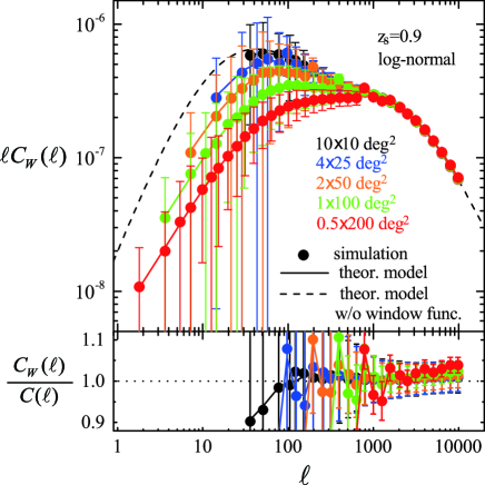
Figure 1: The window-convolved power spectra of the log-normal lensing field for different survey geometries, but keeping the area fixed to 100 deg². As denoted by legend, the circle points are the average power spectra from the 1000 simulation maps (see Section 2.2), for geometries of $10\times 10$ (black points), $4\times 25$ (blue), $2\times 50$ (orange), $1\times 100$ (green) and $0.5\times 200$ deg² (red), from top to bottom points at $\ell\simeq 50$. The error bar around each point denotes $\pm 1\sigma$ scatters of the 1000 realizations. For illustrative purpose, we here plot $\ell C_{W}(\ell)$, making the power spectra amplitude relatively scale-independent over a range of $\ell=[1,10^{4}]$. For comparison, the dashed curve shows the underlying true spectrum without the window function convolution. The solid curve around each point shows the analytical prediction, computed from Eq. (13). The lower panel shows the fractional difference of each power spectrum compared to the true power spectrum, where the $y$-axis plotted range is chosen to illuminate the difference in the range of $\ell>100$.

In this subsection, we test the analytical model of the power spectrum covariance against the simulation of the 1000 convergence maps in Section 2.2.

Before going to the comparison, Fig. 1 shows the window-convolved power spectra for different survey geometries, with the area being fixed to $100$ sq. degrees. We consider a square shape ($10\times 10$  deg²) and rectangular shaped geometries with various side length ratios; $4\times 25$, $2\times 50$, $1\times 100$ and $0.5\times 200~{}$deg², respectively. For the discrete Fourier decomposition, we apply FFT to the rectangular shaped region where $W({\boldsymbol{\theta}})=1$. The different geometries thus have different Fourier resolution as follows. Let us denote the survey geometry as $\Omega_{W}=a\times b$, where $a$ (radian) is the longer side length and $b$ (radian) is the shorter side; e.g., $a=100\times\pi/180=1.75$ rad and $b=0.0175$ rad for the case of $1\times 100$ deg². Thus the fundamental Fourier mode is $\ell_{f}=2\pi/a$ or $2\pi/b$ along the $a$- or $b$-direction, respectively, meaning a finer Fourier resolution along the $a$-direction. However, since all the simulated maps have the same grid scale of $1$ arcmin, the Nyquist frequency (the maximum multipole probed) is the same, $\ell_{\rm Ny}=\pi/1~{}{\rm arcmin}=10800$, for all the survey geometries. The window convolution mixes different Fourier modes, causing extra correlations between different bins. As can be found from Fig. 1, the convolution causes a significant change in the convolved power spectrum compared to the underlying true spectrum at multipoles $\ell\lower 2.15277pt\hbox{$\;\buildrel<\over{\sim}\;$}2\pi/b$. The change is more significant and appears up to higher multipoles for a more elongated survey geometry, due to a greater mixture of different Fourier modes. At larger multipole bins $\ell\lower 2.15277pt\hbox{$\;\buildrel>\over{\sim}\;$}2\pi/b$, the window function stays constant within the multipole bin and all the convolved power spectra appear similar to each other to within 5 per cent. The solid curves are the analytical predictions computed from Eq. (13). Thus the convolved power spectrum can be analytically computed if the window function is known. As can be found from the lower panel, the scatter around each point, computed from the 1000 realizations, is smaller for a more elongated survey geometry, as we will further study below.

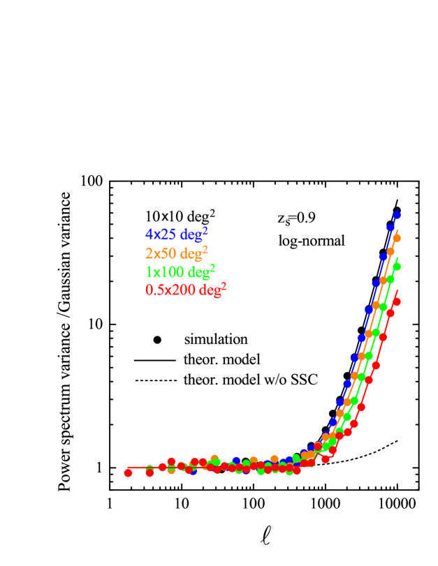
Figure 2: The diagonal elements of the power spectrum covariance for the log-normal convergence field, for different survey geometries as in Fig. 1. Here we plot the diagonal elements relative to the Gaussian covariance, ${\cal C}^{W}(\ell,\ell)/[2C_{W}(\ell)^{2}/N_{\ell}]$; a deviation from unity is due to the non-Gaussian covariance contribution. The symbols are the simulation results, while the solid curves are the analytical predictions computed from Eq.(18), which show a remarkably nice agreement with the simulation results. The dashed curve is the analytical prediction without the super sample covariance (SSC) contribution (the third term in Eq. 18). Thus the non-Gaussian covariance contribution is mainly from the SSC effect.

survey geometry	$(\sigma_{W})^{2}$
$10\times 10~{}{\rm deg}^{2}$	$8.7\times 10^{-7}$
$4\times 25~{}{\rm deg}^{2}$	$7.3\times 10^{-7}$
$2\times 50~{}{\rm deg}^{2}$	$5.2\times 10^{-7}$
$1\times 100~{}{\rm deg}^{2}$	$3.3\times 10^{-7}$
$0.5\times 200~{}{\rm deg}^{2}$	$1.9\times 10^{-7}$

Table 1: The variance of the background convergence mode, $(\sigma_{W})^{2}$ (Eq. 22), for different rectangular geometries, with a fixed survey area of 100 sq. degrees as in Fig. 1. The more elongated geometry has the smaller $(\sigma_{W})^{2}$ for the lensing power spectrum of $\Lambda$CDM model.

In Fig.2, we study the diagonal components of the window-convolved power spectrum covariance as a function of the multipole bins, for different survey geometries as in Fig. 1. Here we plot the diagonal covariance components relative to the Gaussian covariance (the first term of Eq. 18). Hence when the curve deviates from unity in the $y$-axis, it is from the non-Gaussian covariance contribution (the 2nd and 3rd terms in Eq. 18). The log-normal model predicts significant non-Gaussian contributions at $\ell\lower 2.15277pt\hbox{$\;\buildrel>\over{\sim}\;$}$ a few $10^{2}$. Although the relative importance of the non-Gaussian covariance depends on the bin width on which the Gaussian covariance term depends via $N_{\ell_{i}}(\propto 2\pi\ell_{i}\Delta\ell)$, an amount of the non-Gaussian contribution in the log-normal model is indeed similar to that seen from the ray-tracing simulations in Sato et al. (2009) as we will again discuss later.

Fig. 2 shows a significant difference for different survey geometries at $\ell\lower 2.15277pt\hbox{$\;\buildrel>\over{\sim}\;$}$ a few $10^{2}$. Recalling that the window-convolved spectra for different geometries are similar at $\ell\lower 2.15277pt\hbox{$\;\buildrel>\over{\sim}\;$}$a few $10^{2}$ as shown in Fig. 1, we can find that the difference is due to the different SSC contributions, because the survey geometry dependence arises mainly from the SSC term via $(\sigma_{W})^{2}$ in Eq. (18). The most elongated rectangular geometry of $0.5\times 200$ deg² shows a factor $4$ smaller covariance amplitude than the square-shaped geometry of $10\times 10$ deg², the most compact geometry among the 5 geometries considered here. This can be confirmed by the analytical model of the power spectrum covariance; the solid curves, computed based on Eq. (18), show remarkably nice agreement with the simulation results . Table 1 clearly shows that $(\sigma_{W})^{2}$ for the elongated rectangular geometry of $0.5\times 200$ deg² is about factor 4 smaller than that for the square-shaped geometry of $10\times 10$ deg², which explains the relative differences in Fig. 2. For comparison, the dotted curve in the figure shows the analytical prediction if the SSC term, ${\cal C}^{\rm SSC}_{ii}$, is ignored (in this case no difference for different geometries). The analytical model without the SSC term significantly underestimates the simulation results at the nonlinear scales.

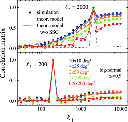
Figure 3: The off-diagonal elements of the power spectrum covariance matrix, for the different survey geometries as in the previous figure. Here we plot the correlation coefficient matrix, $r(\ell_{1},\ell_{2})$ (Eq. 26) as a function of $\ell_{1}$ for $\ell_{2}=2000$ (upper panel) or $200$ (lower). The symbols are the simulation results, while the solid curves are the analytical predictions (Eq. 18); the two are in nice agreement with each other. The dotted curve is the analytical prediction without the SSC effect.

Fig.3 shows the off-diagonal elements of the covariance matrix. For illustrative purpose, we study the correlation coefficients defined as

$$r(\ell_{1},\ell_{2})\equiv\frac{{\cal C}^{W}(\ell_{1},\ell_{2})}{\sqrt{{\cal C}^{W}(\ell_{1},\ell_{1}){\cal C}^{W}(\ell_{2},\ell_{2})}}.$$ (26)

The correlation coefficients are normalized so that $r(\ell_{1},\ell_{2})=1$ for the diagonal components with $\ell_{1}=\ell_{2}$. For the off-diagonal components with $\ell_{1}\neq\ell_{2}$, $r\rightarrow 1$ implies strong correlation between the power spectra of the two bins, while $r=0$ corresponds to no correlation. The figure again shows a significant correlation between the different multipole bins for $\ell_{2}=2000$, due to the significant SSC contribution. Similarly to Fig. 2, the analytical model nicely reproduces the simulation results over the range of multipoles and for the different geometries. For comparison, the dotted curve shows the prediction without the SSC term. As clearly seen from the figure, the correlation is smaller for more elongated survey geometry, due to the smaller $(\sigma_{W})^{2}$ (see Table 1).

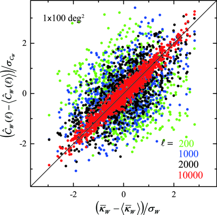
Figure 4: Scatters between the band power of the power spectrum at each multipole bin, $\hat{C}_{W}(\ell)$, and the mean convergence of the survey region, $\bar{\kappa}_{W}$, in the 1000 realizations, for the rectangular survey geometry of $1\times 100$ deg² in Fig. 1. For the higher multipoles $\ell\geq 1000$, the two scatters display a tight relation well approximated by $\left[\hat{C}_{W}(\ell)-\left\langle\hat{C}_{W}(\ell)\right\rangle\right]/\sigma_{C_{W}}=\left[\bar{\kappa}_{W}-\left\langle\bar{\kappa}_{W}\right\rangle\right]/\sigma_{W}$, where $\sigma_{C_{W}}$ and $\sigma_{W}$ are the variances computed from the same $1000$ realizations. Note $\left\langle\bar{\kappa}_{W}\right\rangle\simeq 0$.

As we mentioned below Eq. (25), the approximation we used for the analytical model of the SSC effect is that we modeled the super-survey modes by the mean density fluctuation in each survey realization, $\bar{\kappa}_{W}$. To test the validity of this approximation, in Fig. 4 we study how a scatter of the power spectrum estimation in each realization, $\hat{C}_{W}(\ell)$, is correlated with the mean density in the realization, $\bar{\kappa}_{W}$. Here we used the 1000 realizations for the rectangular geometry of $1\times 100$ deg² as in Fig. 1, but checked that the results are similar for other geometries. For the higher multipoles in the nonlinear regime, $\ell\geq 1000$, the scatters of the two quantities display a tight correlation reflecting the fact that the mean density fluctuation is a main source of the scatters of the band power on each realization basis. In other words, the higher-order super-survey modes such as the gradient and tidal fields that have scale-dependent variations across the survey region are not a significant source of the scatter in the power spectrum; also see Fig. 6 in Li et al. (2014a) and Figs. 2 and 3 in Li et al. (2014b) for the similar discussion. We have also checked that the averaged relation of the scatters is well described by the power spectrum response as implied by Eq. (25): $\left[\hat{C}_{W}(\ell)-\left\langle\hat{C}_{W}(\ell)\right\rangle\right]\simeq(\partial C_{W}(\ell)/\partial\bar{\kappa}_{W})\bar{\kappa}_{W}=(2/\kappa_{0})C_{W}(\ell)\bar{\kappa}_{W}$. The tight relation is probably due to the fact that the power spectrum at a given multipole bin $\ell$ is estimated from the angle average of the Fourier coefficients $|\tilde{\kappa_{{\boldsymbol{\ell}}}}|^{2}$ with the fixed length $|{\boldsymbol{\ell}}|$ and therefore is sensitive to the angle-averaged super-survey modes, i.e. the mean density fluctuation on each realization basis. With this result, an optimal survey geometry or strategy for mitigating the SSC contamination can be studied by monitoring the mean density field $\bar{\kappa}_{W}$ or the variance $\sigma_{W}^{2}$ against survey geometry, and therefore the optimal survey geometry we will show below is valid even on each realization basis. We would like to note that the higher-order correlation function such as the bispectrum may display a sensitivity to the higher-order super-survey modes. This is beyond the scope of this paper, and needs to be further studied.

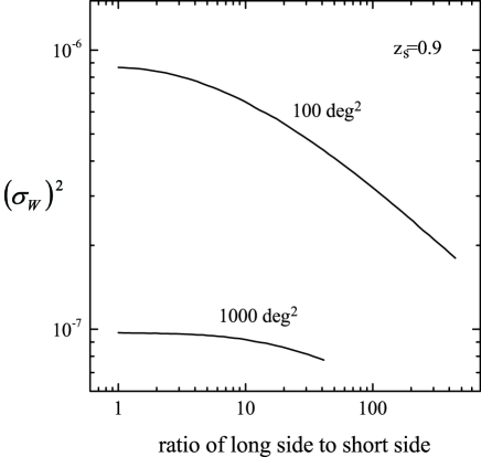
Figure 5: The variance of the background convergence mode, $(\sigma_{W})^{2}$, as a function of the side length ratio for rectangular survey geometry of 100 or 1000 sq. degrees. The more elongated geometry (the greater ratio) has the smaller $(\sigma_{W})^{2}$.

Does the more elongated geometry for a fixed area always have the smaller SSC contribution? The answer is yes for a continuous survey geometry, as can be found from Fig. 5. For the lensing field expected for a $\Lambda$CDM model, the variance of the background convergence modes, $(\sigma_{W})^{2}$, becomes smaller for the more elongated geometry. For a statistically isotropic and homogeneous field, the impact of the non-Gaussian covariance can be mitigated, as long as Fourier modes along the longer side length direction can be sampled, even if the modes the shorter side direction is totally missed. This conclusion is perhaps counter-intuitive, but this is a consequence of non-Gaussian features in non-linear structure formation of a $\Lambda$CDM model.

3 Results

In this section, we study the impact of different survey geometries on the lensing power spectrum measurement, using the simulated maps of log-normal lensing field. In studying this, we do not consider any observational effect: intrinsic shape noise and imperfect shape measurement error. We focus on the effect of survey geometry for clarity of presentation.

3.1 Signal-to-Noise Ratio

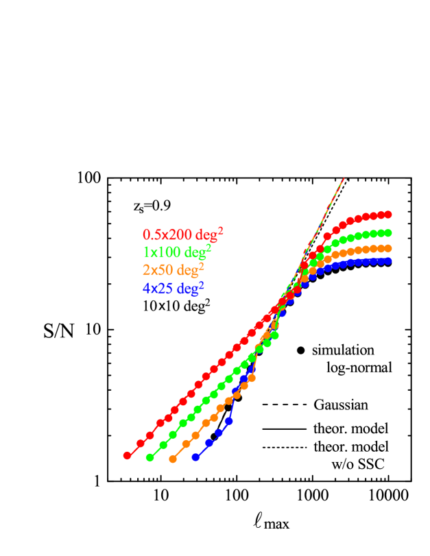
Figure 6: The cumulative signal-to-noise ratio ($S/N$) of the power spectrum measurement, integrated up to a certain maximum multipole ($\ell_{\rm max}$), for different survey geometries as in Fig. 1. The minimum multipole for the different geometries is taken from the fundamental Fourier mode available from each geometry. The symbols show the simulation results; the most elongated geometry gives the highest $S/N$ values over the range of multipoles we consider. The dashed curves show the $S/N$ value expected in a Gaussian field for each geometry, which we estimated by counting the number of Fourier modes around each multipole bin (see text for details). For comparison, the solid and dotted curves show the analytical prediction with and without the SSC effect. The solid curves overlap the dashed curves in the linear regime ($\ell<$ a few $10^{2}$).

Fig. 6 shows the cumulative signal-to-noise ratio ($S/N$) of the window-convolved power spectrum, integrated up to a certain maximum multipole $\ell_{\rm max}$ (Eq. 12), for different survey geometries studied in Fig. 1. The $S/N$ is independent of the bin width and quantifies the total information content inherent in the power spectrum measurement taking into account cross-correlations between the different multipole bins. For the minimum multipole $\ell_{\rm min}$, we adopt the fundamental mode of a given survey geometry ($\ell_{\rm min}=2\pi/a$ as we discussed above). The inverse of $S/N$ gives the fractional error of estimation of the power spectrum amplitude parameter when using the power spectrum information up to $\ell_{\rm max}$ for a given survey, assuming that the shape of the power spectrum is perfectly known. Fig. 6 clearly shows that the $S/N$ significantly varies with different survey geometries, over the range of multipoles. To understand the results, again let us denote the geometry as $\Omega_{W}=a\times b$ ($a$ is the longer side length as before). For the range of multipole bins, $2\pi/a\lower 2.15277pt\hbox{$\;\buildrel<\over{\sim}\;$}\ell\lower 2.15277pt\hbox{$\;\buildrel<\over{\sim}\;$}2\pi/b$, only Fourier modes along the $a$-direction are sampled, therefore this regime is one-dimensional, rather than two-dimensional. Hence, when measuring the power spectrum around a certain $\ell$-bin with the bin width $\Delta\ell$, the number of the sampled modes is given as $N_{\ell}\simeq\Delta\ell/(2\pi/a)$. For the bins $\ell\lower 2.15277pt\hbox{$\;\buildrel>\over{\sim}\;$}\pi/b$, the Fourier modes in the two-dimensional space can be sampled. Hence the number of modes around the $\ell$-bin, $N_{\ell}\simeq 2\pi\ell\Delta\ell/[(2\pi)^{2}/(ab)]=2\pi\ell\Delta\ell/[(2\pi)^{2}/\Omega_{W}]$. The dashed curves give the $S/N$ values expected for a Gaussian field, estimated by accounting for the number of Fourier modes for each survey geometry. To be more precise, the Gaussian covariance is given by ${\cal C}^{G}(\ell,\ell)=2C_{W}(\ell)^{2}/N_{\ell}$ and therefore $(S/N)^{2}=\sum_{\ell}^{\ell_{\rm max}}N_{\ell}/2$. Since we adopt the logarithmically-spaced bins of $\ell_{\rm max}$, the Gaussian predictions $(S/N)^{2}\propto\ell_{\rm max}$ at $\ell_{\rm max}\lower 2.15277pt\hbox{$\;\buildrel<\over{\sim}\;$}2\pi/b$, while $(S/N)^{2}\propto\ell_{\rm max}^{2}$ at $\ell_{\rm max}\lower 2.15277pt\hbox{$\;\buildrel>\over{\sim}\;$}2\pi/b$. The Gaussian prediction shows a nice agreement with the simulation results in the linear regime, $\ell_{\rm max}\lower 2.15277pt\hbox{$\;\buildrel<\over{\sim}\;$}$ a few $10^{2}$. In the linear regime, the figure shows a greater $(S/N)^{2}$ for a more elongated geometry due to the larger $N_{\ell}$. It is also worth noting that the elongated geometry allows for an access to the larger angular scales (i.e. the lower multipoles).

For the regime of large multipoles, $\ell_{\rm max}>$ a few $10^{2}$, the non-Gaussian covariance significantly degrades the information content compared to the Gaussian expectation. The $S/N$ value does not increase at $\ell\lower 2.15277pt\hbox{$\;\buildrel>\over{\sim}\;$}$a few $10^{3}$, implying that the power spectrum can not extract all the information in the log-normal field, i.e. the Gaussian information content from which the log-normal map is generated. The degradation is mainly due to the SSC effect, as shown by the dotted curve (also see Figs. 2 and 3). The more elongated survey geometry mitigates the SSC effect; the most elongated survey geometry of $0.5\times 200$ deg² gives about factor 2 higher $S/N$ than in the most compact square geometry of $10\times 10$ deg². Although we here used the 1000 realizations to compute the $S/N$ values, we have checked that the analytical model in Section 2.3 can reproduce the simulation results.

We have so far used the log-normal convergence field, as an approximated working example of the nonlinear large-scale structure for a $\Lambda$CDM model. In Appendix B, using the 1000 realizations of ray-tracing simulations in Sato et al. (2009), each of which has much smaller area ($25~{}$deg²) and was built based on $N$-body simulations of $\Lambda$CDM model, we also found that an elongated survey geometry gives a larger $S/N$ value compared to a square shape, although the geometry size is limited to a much smaller area, $\Omega_{W}\simeq 0.39~{}$deg², due to the available area sampled from the ray-tracing simulation area ($25$ deg²).

3.2 An implication for cosmological parameter estimation

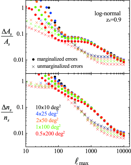
Figure 7: The fractional error of cosmological parameters, the primordial power spectrum amplitude $A_{s}$ (upper panel) and the spectral tilt parameter $n_{s}$ (lower), expected from the power spectrum measurement for different survey geometries, but for a fixed survey area of $100$ sq. degrees (see text for the details). Note that the other cosmological parameters are fixed to their fiducial values. The error is shown as a function of the maximum multipole $\ell_{\rm max}$ up to which the power spectrum information is included in the parameter forecast. The filled circle symbols are the marginalized errors, while the cross symbols denote the unmarginalized errors, the error when another parameter (another $n_{s}$ or $A_{s}$) is fixed to the fiducial value.

What is the impact of survey geometry on cosmological parameter estimation? Can we achieve a higher precision of cosmological parameters by just taking an optimal survey geometry, for a fixed area (although we here consider a continuous survey geometry)? The SSC causes correlated up- or down-scatters in the power spectrum amplitudes over a wide range of multipole bins. The correlated scatters to some extent preserve a shape of the power spectrum, compared to random scatters over different bins. Hence, the SSC is likely to most affect parameters that are sensitive to the power spectrum amplitude, e.g. the primordial curvature perturbation $A_{s}$. On the other hand, other parameters that are sensitive to the shape, e.g. the spectral tilt of the primordial power spectrum $n_{s}$, is less affected by the SSC (see also Takada & Jain 2009; Li et al. 2014b, for the similar discussion).

Based on this motivation, we use the simulated log-normal convergence maps to estimate an expected accuracy of the parameters ($A_{s}$, $n_{s}$) as a function of different survey geometries, using the Fisher information matrix formalism. When including the power spectrum information up to a certain maximum multipole $\ell_{\rm max}$, the Fisher matrix for the two parameters is given as

$$F_{ab}({\boldsymbol{\lambda}})=\sum_{\ell_{i},\ell_{j}\leq\ell_{\rm max}}\frac{\partial\ln C_{W}(\ell_{i};{\boldsymbol{\lambda}})}{\partial\ln\lambda_{a}}\left[{\boldsymbol{{\cal C}}}^{W}\right]^{-1}_{\ell_{i}\ell_{j}}\frac{\partial\ln C_{W}(\ell_{j};{\boldsymbol{\lambda}})}{\partial\ln\lambda_{b}},$$ (27)

where $\lambda_{a}$ denote the $a$-th parameter; $\lambda_{1}=A_{s}$ or $\lambda_{2}=n_{s}$ in our definition. Note that we consider the window-convolved power spectrum as the observable. To calculate the power spectrum derivative, $\partial C_{W}(\ell)/\partial\ln\lambda_{a}$, we generated 100 realizations of the convergence maps, which are built based on the input linear power spectrum with $\pm 5\%$ change of $\lambda_{a}$ on each side from its fiducial value (therefore 200 realizations in total). Then we evaluated the window-convolved power spectrum from the average of the realizations, and used the spectra to evaluate the derivatives $\partial C_{W}(\ell)/\partial\ln\lambda_{a}$ from the two-side numerical differentiation method. The fractional error on each parameter including marginalization over uncertainties of other parameter is given by $\Delta\lambda_{a}/\lambda_{a}=\sqrt{[{\boldsymbol{F}}]^{-1}_{aa}}$, where $[{\boldsymbol{F}}]^{-1}$ is the inverse of the Fisher matrix.

Fig. 7 shows the errors of each parameter ($A_{s}$ or $n_{s}$) expected for a hypothetical survey with 100 sq. degrees, but assuming different survey geometries as in Fig. 1. As expected from the results of $S/N$ in Fig. 6, the most elongated geometry allows the highest accuracy of these parameters over the range of $\ell_{\rm max}$ we consider. To be more precise, the elongated geometry of $0.5\times 200$ deg² gives about 3 or 25% improvement in the marginalized or unmarginalized error of $A_{s}$ at $\ell_{\rm max}\simeq 2000$, respectively, compared to the square geometry of $10\times 10$ deg². For $n_{s}$ the elongated geometry gives almost the same marginalized error (more exactly speaking, 0.3% degraded error) and about 20% improvement for the unmarginalized error at $\ell_{\rm max}\simeq 2000$. Thus the improvement in the error of $A_{s}$ is greater than that in the error of $n_{s}$. However, the improvement in the marginalized error is milder compared to that in the unmarginalized error or the $S/N$ value, for $\ell_{\rm max}\lower 2.15277pt\hbox{$\;\buildrel>\over{\sim}\;$}$a few $10^{3}$. Since the $S/N$ value is proportional to the volume of Fisher ellipse in a multidimensional parameter space, the marginalized error is obtained from the projection of the Fisher ellipse onto the parameter axis, yielding a smaller improvement in the marginalized error (see Takada & Jain 2009, for the similar discussion).

4 Sparse sampling optimization of the survey geometry

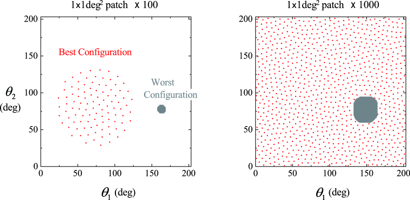
Figure 8: The sparse-sampling strategy for the survey footprints when the total area is fixed. The range shown is the all-sky map ($203\times 203$ sq. degrees) assuming the flat-sky approximation. Note that we assumed the periodic boundary condition beyond $203$ degrees. Assuming that the fundamental building block of the survey footprints is a square patch of $1\times 1$ sq. degrees, we address which configuration of the $N_{\rm p}$ patches is best or worst in a sense that the configuration has the smallest or largest SSC contamination, for the fixed total area of 100 (left panel) or 1000 (right) sq. degrees. For illustrative purpose, the best and worst configurations are plotted within the same panel (in the right panel, the other patches are similarly distributed under the worst configuration). Because of the periodic boundary condition, the center position of each configuration can be displaced in parallel. For the best configuration, the different patches are separated by about 15 degrees from each other. The angular extent of all the patches is found to be about 10000 sq. degrees or all sky ($203\times 203$ sq. degrees), respectively. The worst configuration is close to the square shape, with slightly rounded corners.

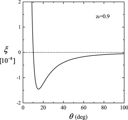
Figure 9: The two-point correlation function of the log-normal convergence field, $\xi(\theta)$, for source redshift $z_{s}=0.9$. The two-point function has a negative minimum at about 15 degrees, which corresponds to the separation between the different patches for the best configuration in Fig. 8.

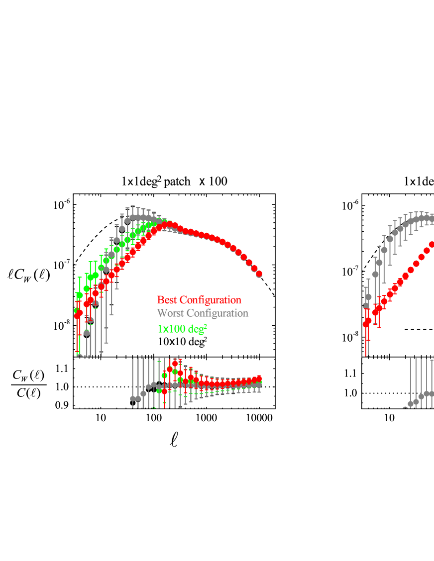
Figure 10: The window-convolved power spectra for the best or worst configuration for the fixed area of 100 or 1000 sq. degrees, for the sparse-sampling strategy as in Fig. 8. In the left panel, for comparison, we also show the result for the rectangular survey geometry of $1\times 100$ sq. degrees (green) and the square geometry of $10\times 10$ sq. degrees (black) in Fig. 1. The error bar around each point denotes the $\pm 1\sigma$ scatters among the 1000 realizations, clearly showing that the scatter for the best configuration is smaller than that for the worst configuration. The dashed curve is the true power spectrum. The lower plot shows the fractional difference compared to the true spectrum as in Fig. 1.

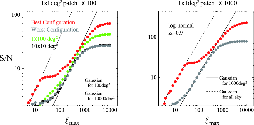
Figure 11: The cumulative $S/N$ for the best or worst configurations in Fig. 8. In the left panel, for comparison, we also show the results for the rectangular geometries of $1\times 100$ or $10\times 10$ sq. degrees. The dashed curve in each panel shows the $S/N$ value expected for a Gaussian field in the “sparse-sampling” regime, where we assumed the angular extent of the best configuration, $100$ or $203\times 203$ (all-sky) sq. degrees, as the “effective” survey area, respectively. To be more precise, we used the total number of Fourier modes around each multipole bin assuming the effective survey area: $N_{\ell}=2\pi\ell\Delta\ell/[(2\pi)^{2}/\Omega_{\rm eff}]$ and $\Omega_{\rm eff}$ is the effective area. On the other hand, the solid curve is the Gaussian prediction in the patch-inside regime, i.e. the value obtained assuming the actual survey area, $100$ or 1000 sq. degrees. In the intermediate multipole range between the two regimes, the $S/N$ value appears to be constant, as no Fourier mode is sampled in this configuration. Nevertheless, the figure shows that the best configuration has the greater $S/N$ values over the wide range of multipoles.

We have so far considered a continuous geometry. In this section, we explore an optimal sparse-sampling strategy. In this case the window function becomes even more complicated, causing a greater mixture between different Fourier modes over a wider range. Observationally, a continuous geometry might be to some extent preferred. There are instances, where we want to avoid the mode coupling due to the window function, especially in the presence of inhomogeneous selection function over different pointings of a telescope. There are also instances, where we want to build a continuous survey region by tiling different patches with an overlap between different pointings, because such a strategy allows a better photometry calibration by comparing the measured fluxes of the same objects in the overlapping regions across the entire survey region (Padmanabhan et al. 2008). In addition the sparse sampling of the survey strategy may require a more slewing of a telescope to cover separated regions, which may cause an extra overhead and therefore lower a survey efficiency for a given total amount of the allocated observation time. There are also instances, where we require a minimum size of a connected region in order to have a sufficient sampling of the particular Fourier mode such as the baryonic acoustic oscillation scale. Here we ignore these possible observational disadvantages of a sparse sampling strategy. Instead we here address a question: what is the best sparse-sampling strategy for maximizing the information content of the power spectrum measurement for a fixed survey area?

Again recalling that the degradation in the power spectrum measurement is mainly caused by the SSC effect, we can find the answer to the above question by searching for a disconnected geometry that minimizes $(\sigma_{W})^{2}$ in Eq. (18). For comparison, we also search for the worst survey geometry in a sense that it gives the lowest information content. To find these geometries, we employ the following method. First, we divide each map of the log-normal lensing field ($203\times 203~{}{\rm deg}^{2}$) into $203\times 203$ patches, i.e. each patch has an area of 1 sq. degrees. Thus we consider each patch as the fundamental building block of survey footprints for an assumed survey area. The Subaru HSC has a FoV of about 1.7 sq. degrees, so one may consider the FoV size of a telescope for the patch. The following discussion can be applied for any other size of the patch.

In the following we assume either 100 or 1000 sq. degrees for the total area, and then numerically search for configurations of the 100 or 1000 patches which have the smallest or largest $(\sigma_{W})^{2}$ value. The numerical procedures are:

• Generate a random distribution of the $N_{\rm p}$ ($=100$ or $1000$) patches in the entire map ($203\times 203$ patches in total).

• Allow the $i$-th patch’s position to move to an unfilled patch, with fixing other patches’ positions, until the $i$-th patch’s position yields the minimum or maximum value $(\sigma_{W})^{2}$ computed from the total window function of $N_{\rm p}$ patches based on Eq. (22).

• Repeat the procedure (ii) for each of other patches iteratively (we may come back to the $i$-th patch) until the minimum or maximum $(\sigma_{W})^{2}$ value is well converged.

• Redo the procedures (i)-(iii) from different initial distributions of the $N_{\rm p}$ patches.

We used $10^{4}$ initial positions. In the following, we show the results for the best and worst configurations obtained from the 10⁴ initial positions, but we checked that the different initial positions give almost the same configurations.

To make a fair comparison between different configurations/geometries, we use the Fourier transform of the entire map region ($203\times 203$ deg²); the patches outside the survey footprints or the unfilled patches are zero-padded (i.e. set to $\kappa({\boldsymbol{\theta}})=0$), and then perform FFT with $12180^{2}$ grids to compute the Fourier-transformed field. In this way, the fundamental Fourier mode (Fourier resolution) and the maximum Fourier mode are the same for all the survey geometries.

Fig.8 shows the best and worst configurations of the survey footprints for each of 100 or 1000 sq. degrees, respectively. The best (worst) configuration has $(\sigma_{W})^{2}=1.3\times 10^{-7}$ ($8.8\times 10^{-7}$) for $100~{}{\rm deg}^{2}$ or $1.1\times 10^{-8}$ ($1.0\times 10^{-7}$) for $1000~{}{\rm deg}^{2}$, respectively. For the best configuration, the distribution of the $N_{\rm p}$ patches (each $1\times 1$ sq. degrees) appears regularly spaced, separated by $\sim$15 deg. from each other, rather than random, as discussed below. The angular extent of the best configuration is about 10000 sq. degrees or all-sky area (about 41000 sq. degrees) for the case of 100 or 1000 sq. degrees, respectively. Thus the filling fraction is only 1 or 2.4 per cent, respectively. Hence the sparse-sampling strategy might allow for about factor 100 faster survey speed (equivalently factor 100 less telescope time), compared to the 100 per cent filling strategy. On the other hand, the worst configuration is almost square shaped, with slightly rounded corners.

To gain a more physical understanding of Fig. 8, we can rewrite Eq. (23) for $(\sigma_{W})^{2}$ as

$$\left(\sigma_{W}\right)^{2}=\frac{1}{\Omega_{W}^{2}}\sum_{i=1}^{N_{p}}\int\!d^{2}{\boldsymbol{\theta}}\!\int\!d^{2}{\boldsymbol{\theta}}^{\prime}\,W_{i}({\boldsymbol{\theta}})W_{i}({\boldsymbol{\theta}}^{\prime})\xi(|{\boldsymbol{\theta}}-{\boldsymbol{\theta}}^{\prime}|)$$

$$+\frac{2}{\Omega_{W}^{2}}\sum_{i,j;i>j}\int\!d^{2}{\boldsymbol{\theta}}\!\int\!d^{2}{\boldsymbol{\theta}}^{\prime}\,W_{i}({\boldsymbol{\theta}})W_{j}({\boldsymbol{\theta}}^{\prime})\xi(|{\boldsymbol{\theta}}-{\boldsymbol{\theta}}^{\prime}|),$$ (28)

where we re-defined the window function as $W({\boldsymbol{\theta}})=\sum_{i}W_{i}({\boldsymbol{\theta}})$, and $W_{i}({\boldsymbol{\theta}})$ is the window function of the $i$-th patch. Since $W_{i}({\boldsymbol{\theta}})=1$ when ${\boldsymbol{\theta}}$ is inside the $i$-th patch, otherwise $W_{i}({\boldsymbol{\theta}})=0$, the first term arises from the integration of $\xi(|{\boldsymbol{\theta}}-{\boldsymbol{\theta}}^{\prime}|)$ when the vectors ${\boldsymbol{\theta}}$ and ${\boldsymbol{\theta}}^{\prime}$ are in the same patch. One the other hand, the second term arises form the integration of $\xi(|{\boldsymbol{\theta}}-{\boldsymbol{\theta}}^{\prime}|)$ when the vector ${\boldsymbol{\theta}}$ and ${\boldsymbol{\theta}}^{\prime}$ are in the different patches. As can be found from Fig. 9, the first term is always positive-additive, while the second term can have a negative contribution, lowering $(\sigma_{W})^{2}$, when the separation of different patches is more than $\sim$10 deg. Since $\xi(r)$ has a negative minimum at $r\sim 15$ deg., $(\sigma_{W})^{2}$ can be minimized if taking a configuration so that different patches are separated by $\sim$15 deg. from each other. Thus, even if different patches are separated by an infinite angle, i.e. $\xi=0$, such a configuration does not have the smaller $(\sigma_{W})^{2}$.

In Fig. 10 we show the window-convolved power spectra for the best and worst configurations. Compared to the true power spectrum, the sparse sampling causes a significant change in the convolved spectrum at $\ell\lower 2.15277pt\hbox{$\;\buildrel<\over{\sim}\;$}$a few $10^{2}$, due to a significant transfer of Fourier modes due to the complex window function. Here the multipole scale of a few $10^{2}$ corresponds to the patch size ($1\times 1$ deg²), the fundamental block of the survey footprints. At multipoles $\ell\lower 2.15277pt\hbox{$\;\buildrel>\over{\sim}\;$}$ a few $10^{2}$, the convolved power spectra become similar to the true spectrum to within 5 per cent in the amplitude. As can be found from the lower panel, the best configuration clearly shows the smaller scatter at each multipole bin among the 1000 realizations than that of the worst configuration or more generally a compact geometry.

Fig. 11 shows the cumulative $S/N$ for the best and worst configurations of 100 or 1000 sq. deg. area in Fig. 8. The best configuration allows a higher $S/N$ of the power spectrum measurement over the range of multipoles, from the linear to non-linear regimes. Thus the sparse sampling allows an access to the larger angular (lower multipole) scales (Kaiser 1998). For the case of 100 sq. degrees (the left panel in Fig. 8), the angular extent of the different patches is about 10000 sq. degrees (or 100 deg. on a side). The figure shows that the $S/N$ is close to the Gaussian expectation for the effective area, $10000$ sq. degrees or all-sky area in the left or right panels, respectively. To be more precise the covariance matrix in this regime is approximated as ${\cal C}_{ij}=2C_{W}(\ell)^{2}\delta^{K}_{ij}/N_{\ell}$ with $N_{\ell}=2\pi\ell\Delta\ell/[(2\pi)^{2}/\Omega_{\rm eff}]$, where $\Omega_{\rm eff}$ is the effective area.

The sparse-sampling, by construction, can not probe Fourier modes over the range of intermediate angular scales such as $10\lower 2.15277pt\hbox{$\;\buildrel<\over{\sim}\;$}\ell\lower 2.15277pt\hbox{$\;\buildrel<\over{\sim}\;$}$ a few 10² in our case. In this intermediate range, the $S/N$ value is flat and does not increase with increasing $\ell_{\rm max}$. On the other hand, at the angular scales smaller than the patch size ($\ell\lower 2.15277pt\hbox{$\;\buildrel>\over{\sim}\;$}$a few $10^{2}$), the power spectrum measurement arises from Fourier modes inside each patch. At the small scales, the SSC effect becomes significant. The figure clearly shows that the best configuration allows for a factor 2 – 2.5 greater $S/N$ at $\ell_{\rm max}\lower 2.15277pt\hbox{$\;\buildrel>\over{\sim}\;$}10^{3}$ than in the worst configuration. Also notice that, as can be found from the left panel, the best-configuration gives the higher $S/N$ than in the elongated rectangular geometry of $1\times 100$ sq. degrees, whose shortest side length is the same as the patch size. Thus the sparse sampling strategy yields a higher precision of the power spectrum measurement than a continuous geometry, for the fixed total area.

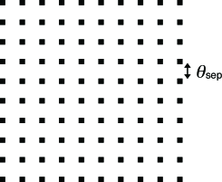
Figure 12: Another working example of the sparse-sampling survey footprints. Assuming that the fundamental building block is the patch $1\times 1$ sq. degrees as in Fig. 8 and the total survey area is 100 sq. degrees (100 patches), we study different configurations of the 100 patches as a function of the separation angle $\theta_{\rm sep}$, as illustrated.

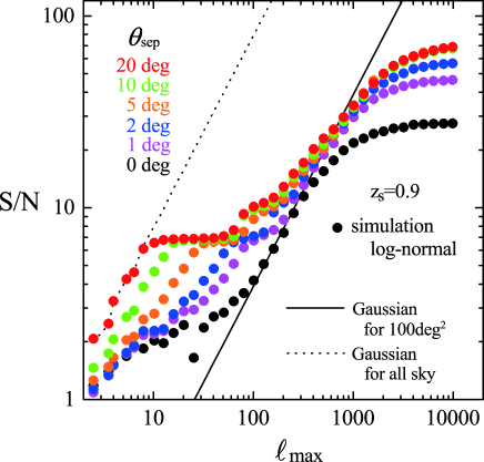
Figure 13: The cumulative $S/N$ for the different configurations as a function of the separation angle $\theta_{\rm sep}$ in Fig. 12. The dotted and solid curves show the $S/N$ values expected for a Gaussian field, for the effective area of $100$ or all sky, respectively.

Finally, we further study the advantage of the sparse sampling strategy for the power spectrum measurement. Assuming that the 100 patches (each patch is $1\times 1$ sq. degrees) is regularly distributed and different patches are regularly separated by the angle $\theta_{\rm sep}$ from each other as given in Fig. 12, Fig. 13 shows how the $S/N$ value of power spectrum measurement changes with the separation angle. The continuous geometry, given by no separation ($\theta_{\rm sep}=0$), yields the smallest $S/N$. The wider separation angle (larger $\theta_{\rm sep}$) allows an access to the Fourier modes over the wider range of multipoles from the linear to nonlinear regimes. If the separation angle is more than $5$ degrees, the SSC effect can be mitigated.

We have so far considered the fixed patch size, $1\times 1$ sq. degrees. We have checked that, if the finer patch size is adopted for the fixed total area, the best configuration further improves the total information content of the power spectrum measurement over the wider range of multipole bins. We also note that the results we have shown qualitatively hold for different source redshifts, $z_{s}=0.6$ – 1.5.

5 Conclusion and Discussion

In this paper we have studied how the accuracy of weak lensing power spectrum measurement varies with different survey geometries. We have used the 1000 realizations of weak lensing maps and the analytical model, assuming the log-normal model that approximates non-Gaussian features seen in the weak lensing field for $\Lambda$CDM model. Since the SSC effect arising from super-survey modes dominates the non-Gaussian covariance in the range of $\ell\simeq 10^{3}$, the key quantity to determine its survey geometry dependence is the variance of the mean convergence mode in the survey region, $(\sigma_{W})^{2}=\left\langle\bar{\kappa}_{W}^{2}\right\rangle$, where $\bar{\kappa}_{W}=(1/\Omega_{S})\int\!d^{2}{\boldsymbol{\theta}}W({\boldsymbol{\theta}})\kappa({\boldsymbol{\theta}})$. We showed that an optimal survey geometry can be found by looking for a geometry to minimize $(\sigma_{W})^{2}$ for a fixed total area. We used the formulation in Takada & Hu (2013) to analytically derive the power spectrum covariance and then used the analytical prediction to confirm the finding from the simulated maps.

We showed that, for a fixed total area, the optimal survey geometry can yield a factor 2 improvement in the cumulative $S/N$ of power spectrum measurement, integrated up to $\ell_{\rm max}\simeq 10^{3}$, compared to the $S/N$ in a compact geometry such as square and circular shaped geometries. Furthermore, by taking a sparse sampling strategy, we can increase the dynamic range of multipoles in the power spectrum measurement, e.g., by a factor 100 in the effective survey area, if the survey field is divided into 100 patches. Again, in this case, the optimal survey design can be found by looking for a configuration of 100 patches to minimize the variance $(\sigma_{W})^{2}$.

Our results might imply an interesting application for upcoming surveys. For example, the LSST or Euclid surveys are aimed at performing an almost all-sky imaging survey. If these surveys adopt a sparse-sampling strategy with a few per cent filling factor in the first few years (Fig. 8), the few per cent data might allow the power spectrum measurements with an equivalent statistical precision to that of the all-year data, i.e. enabling the desired cosmological analysis very quickly. Then it can fill up unobserved fields between the different patches in the following years. Thus, while the same all-sky data is obtained in the end, taking a clever survey strategy over years might allow for a quicker cosmological analysis with the partial data in the early phase of the surveys.

In order to have the improved precision in the power spectrum measurement with the optimal survey design, we need to properly understand the effect of the survey window function. In reality, inhomogeneous depth and masking effects need to be properly taken into account. The sparse sampling causes sidelobes in the Fourier-transformed window function, causing a mixture of different Fourier modes in the power spectrum measurement (also see Kaiser 1998). The effect of the side lobes also needs to be taken into account, when comparing the measurement with theory. Throughout this paper we simply adopted the sharp window function: $W({\boldsymbol{\theta}})=0$ or 1 (see the sentences around Eq. 7). To reduce the mode-coupling due to the sharp window, we may want to use an apodization of the window function, which is an operation to smooth out the sharp window, e.g. with a Gaussian function, in order to filter out high-frequency modes. With such an apodization method, we can make the window-convolved power spectrum closer to the true power spectrum at a given multipole bin, which may be desired in practice when comparing the measured power spectrum with theory. However, the effective survey area decreases and it degrades the extracted information content or the $S/N$ value at the price. Thus an optimal window function needs to be explored depending on scientific goals of a given survey.

Throughout this paper, we have employed the simple log-normal model to approximate the weak lensing field in a $\Lambda$CDM model. We believe that the results we have found are valid even if using the full ray-tracing simulations. However, the brute-force approach requires huge-volume $N$-body simulations to simulate a wide-area weak lensing survey as well as requires the many realizations. This would be computationally expensive. This problem can be studied by using a hybrid method combining the numerical and analytical methods in Li et al. (2014a) and Takada & Hu (2013). Li et al. (2014a, b) showed that a super-box mode can be included by introducing an apparent curvature parameter $\Omega_{K}$, given in terms of the super-box mode $\delta_{b}$, and then solving an evolution of $N$-body particles in the simulation under the modified background expansion. As shown in Takada & Hu (2013), since the dependence of the SSC effect on survey geometry is determined mainly by the variance $(\sigma_{W})^{2}$, we can easily compute the variance by using the analytical prediction for the input linear power spectrum (Eq. 22) or using the simulation realizations of linear convergence field. Thus, by combining these methods, we can make a more rigorous study of the survey geometry optimization for upcoming wide-area surveys, at a reasonable computational expense.

Although we have studied the problem for a two-dimensional weak lensing field, the method in this paper can be applied to a survey optimization problem for a three-dimensional galaxy redshift survey. Again various galaxy redshift surveys are being planned (e.g. Takada et al. 2014), and the projects are expensive both in time and cost, so the optimal survey design is important to explore.

Appendix A Trispectrum of log-normal convergence field

Let us consider the log-normal convergence field $\kappa$: its mean is zero and its statistics is characterized by the two-point correlation function, $\xi_{12}\equiv\xi(|{\boldsymbol{\theta}}_{1}-{\boldsymbol{\theta}}_{2}|)=\langle\kappa({\boldsymbol{\theta}}_{1})\kappa({\boldsymbol{\theta}}_{2})\rangle$. Then, the four-point correlation of $\kappa$ can be written in terms of $\xi$ as (Hilbert et al. 2011),

$$\langle\kappa({\boldsymbol{\theta}}_{1})\kappa({\boldsymbol{\theta}}_{2})\kappa({\boldsymbol{\theta}}_{3})\kappa({\boldsymbol{\theta}}_{4})\rangle=\xi_{12}\xi_{34}+\xi_{13}\xi_{24}+\xi_{14}\xi_{23}+\frac{1}{\kappa_{0}^{2}}\left[\xi_{12}\xi_{13}\xi_{14}+\xi_{12}\xi_{13}\xi_{24}+\xi_{12}\xi_{13}\xi_{34}+\xi_{12}\xi_{14}\xi_{23}+\xi_{12}\xi_{14}\xi_{34}\right.$$

$$~{}+\xi_{12}\xi_{23}\xi_{24}+\xi_{12}\xi_{23}\xi_{34}+\xi_{13}\xi_{14}\xi_{23}+\xi_{13}\xi_{14}\xi_{24}+\xi_{13}\xi_{23}\xi_{24}+\xi_{13}\xi_{23}\xi_{34}+\xi_{14}\xi_{23}\xi_{24}+\xi_{14}\xi_{23}\xi_{34}+\xi_{12}\xi_{24}\xi_{34}$$

$$~{}\left.+\xi_{13}\xi_{24}\xi_{34}+\xi_{14}\xi_{24}\xi_{34}\right]+O\left(\xi^{4}/\kappa_{0}^{4}\right)$$ (29)

The first three terms are disconnected parts, while the others are connected parts which are leading correction terms arising from non-Gaussianity. We ignore the higher-order terms since $\xi/\kappa_{0}^{2}$ is usually very small. This approximation corresponds to “the simplified log-normal approximation” in Hilbert et al. (2011). By performing Fourier transform, we have

$$\langle\tilde{\kappa}({\boldsymbol{\ell}}_{1})\tilde{\kappa}({\boldsymbol{\ell}}_{2})\tilde{\kappa}({\boldsymbol{\ell}}_{3})\tilde{\kappa}({\boldsymbol{\ell}}_{4})\rangle=C(\ell_{1})C(\ell_{3})\delta_{\rm D}^{2}({\boldsymbol{\ell}}_{12})\delta_{\rm D}^{2}({\boldsymbol{\ell}}_{34})+C(\ell_{1})C(\ell_{2})\delta_{\rm D}^{2}({\boldsymbol{\ell}}_{13})\delta_{\rm D}^{2}({\boldsymbol{\ell}}_{24})+C(\ell_{1})C(\ell_{2})\delta_{\rm D}^{2}({\boldsymbol{\ell}}_{14})\delta_{\rm D}^{2}({\boldsymbol{\ell}}_{23})$$

$$~{}+\frac{\left(2\pi\right)^{2}}{\kappa_{0}^{2}}\left[C(\ell_{1})C(\ell_{2})C(\ell_{3})+C(\ell_{1})C(\ell_{2})C(\ell_{4})+C(\ell_{1})C(\ell_{3})C(\ell_{4})+C(\ell_{2})C(\ell_{3})C(\ell_{4})+C(\ell_{2})C(\ell_{4})C(\ell_{12})\right.$$

$$~{}+C(\ell_{2})C(\ell_{3})C(\ell_{12})+C(\ell_{3})C(\ell_{4})C(\ell_{13})+C(\ell_{2})C(\ell_{3})C(\ell_{13})+C(\ell_{3})C(\ell_{4})C(\ell_{14})+C(\ell_{2})C(\ell_{4})C(\ell_{14})$$

$$~{}+C(\ell_{1})C(\ell_{2})C(\ell_{23})+C(\ell_{1})C(\ell_{3})C(\ell_{23})+C(\ell_{1})C(\ell_{2})C(\ell_{24})+C(\ell_{1})C(\ell_{4})C(\ell_{24})+C(\ell_{1})C(\ell_{4})C(\ell_{34})$$

$$~{}\left.+C(\ell_{1})C(\ell_{3})C(\ell_{34})\right]\delta_{\rm D}^{2}({\boldsymbol{\ell}}_{1234})+O\left(C^{4}/\kappa_{0}^{4}\right),$$ (30)

where ${\boldsymbol{\ell}}_{ij}={\boldsymbol{\ell}}_{i}+{\boldsymbol{\ell}}_{j}$ and ${\boldsymbol{\ell}}_{ijkl}={\boldsymbol{\ell}}_{i}+{\boldsymbol{\ell}}_{j}+{\boldsymbol{\ell}}_{k}+{\boldsymbol{\ell}}_{l}$. The trispectrum is defined as the connected part of the above function, $\langle\tilde{\kappa}({\boldsymbol{\ell}}_{1})\tilde{\kappa}({\boldsymbol{\ell}}_{2})\tilde{\kappa}({\boldsymbol{\ell}}_{3})\tilde{\kappa}({\boldsymbol{\ell}}_{4})\rangle_{\rm c}=(2\pi)^{2}T({\boldsymbol{\ell}}_{1},{\boldsymbol{\ell}}_{2},{\boldsymbol{\ell}}_{3},{\boldsymbol{\ell}}_{4})\delta_{\rm D}^{2}({\boldsymbol{\ell}}_{1234})$. Then we have,

$$T({\boldsymbol{\ell}}_{1},{\boldsymbol{\ell}}_{2},{\boldsymbol{\ell}}_{3},{\boldsymbol{\ell}}_{4})=\frac{1}{\kappa_{0}^{2}}\left[C(\ell_{1})C(\ell_{2})C(\ell_{3})+C(\ell_{1})C(\ell_{2})C(\ell_{4})+C(\ell_{1})C(\ell_{3})C(\ell_{4})+C(\ell_{2})C(\ell_{3})C(\ell_{4})\right.$$

$$~{}+C(\ell_{2})C(\ell_{4})C(\ell_{12})+C(\ell_{2})C(\ell_{3})C(\ell_{12})+C(\ell_{3})C(\ell_{4})C(\ell_{13})+C(\ell_{2})C(\ell_{3})C(\ell_{13})+C(\ell_{3})C(\ell_{4})C(\ell_{14})$$

$$~{}+C(\ell_{2})C(\ell_{4})C(\ell_{14})+C(\ell_{1})C(\ell_{2})C(\ell_{23})+C(\ell_{1})C(\ell_{3})C(\ell_{23})+C(\ell_{1})C(\ell_{2})C(\ell_{24})+C(\ell_{1})C(\ell_{4})C(\ell_{24})$$

$$~{}\left.+C(\ell_{1})C(\ell_{4})C(\ell_{34})+C(\ell_{1})C(\ell_{3})C(\ell_{34})\right].$$ (31)

In a particular configuration of ${\boldsymbol{\ell}}_{1}+{\boldsymbol{\ell}}_{2}={\boldsymbol{\ell}}_{3}+{\boldsymbol{\ell}}_{4}=0$, the trispectrum has a simple form,

$$T({\boldsymbol{\ell}}_{1},-{\boldsymbol{\ell}}_{1},{\boldsymbol{\ell}}_{2},-{\boldsymbol{\ell}}_{2})=\frac{1}{\kappa_{0}^{2}}\left[2C(\ell_{1})C(\ell_{2})\left\{C(\ell_{1})+C(\ell_{2})\right\}+\left\{C(\ell_{1})+C(\ell_{2})\right\}^{2}\left\{C(|{\boldsymbol{\ell}}_{1}+{\boldsymbol{\ell}}_{2}|)+C(|{\boldsymbol{\ell}}_{1}-{\boldsymbol{\ell}}_{2}|)\right\}\right].$$ (32)

Appendix B Results: $\Lambda$CDM ray-tracing simulations

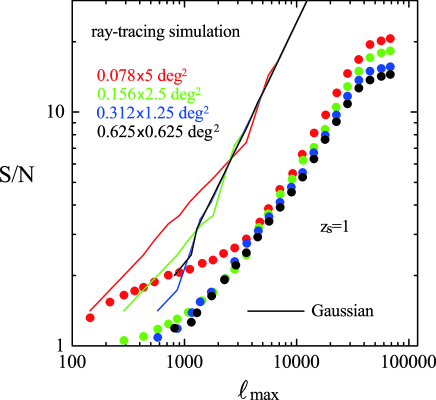
Figure 14: The cumulative $S/N$ measured from the ray-tracing simulations for $\Lambda$CDM model and source redshift $z_{s}=1$, taken from Sato et al. (2009). The different color symbols show the results for different geometries: the square-shaped geometry with area $0.625\times 0.625~{}{\rm deg}^{2}$ (black), and the rectangular-shaped geometries with the same area, but with different side ratios, $0.078\times 5$ (red), $0.156\times 2.5$ (green), and $0.312\times 1.25$ deg² (blue), respectively. The solid curves are the Gaussian error predictions.

In most part of this paper we have used the simulated convergence maps for the log-normal model. Our method allows us to simulate the convergence field over a wide area (all-sky area), thereby including all the Fourier modes from very small scales to all-sky scales, and to simulate many realizations at a computationally cheap cost. However, the log-normal model is an empirical model to mimic the lensing field for a $\Lambda$CDM model. In this appendix we use the ray-tracing simulations in Sato et al. (2009) to study whether the results we show hold for a more realistic lensing field.

Each of the 1000 realizations in Sato et al. (2009) has an area of $5\times 5$ sq. degrees in square shaped geometry, and is given in $2048^{2}$ grids (each grid size is 0.15 arcmin on a side). As can be found from Fig. 1 in Sato et al. (2009), the ray-tracing simulations were done in a light cone of area $5\times 5{\rm deg}^{2}$, viewed from an observer position (z = 0). The projected mass density fields in intermediate-redshift slices were generated from N-body simulations which have a larger simulation box than the volume covered by the light cone. Hence the lensing fields have contributions from the mass density field of scales outside the ray-tracing simulation area, although, exactly speaking, the modes outside the N-body simulation box were not included. Thus the ray-tracing simulations include the SSC effect. As discussed in Section 3 of Sato et al. (2009), the ray-tracing simulation would not be so reliable at $\ell\lower 2.15277pt\hbox{$\;\buildrel>\over{\sim}\;$}6000$ due to the resolution issue of the original N-body simulations. However, since we are interested in the effect of different survey geometries, we below use the simulations down to the pixel scale.

Although the ray-tracing simulation map is in small area ($5\times 5$ deg²), we want to study a wide range of different geometries available from the simulated map. Here we consider a square-shaped geometry of $0.625\times 0.625(=0.39)$ sq. degrees and rectangular-shaped geometries of different side ratios: $0.078\times 5$, $0.156\times 2.5$, and $0.312\times 1.25$ deg², which have the side ratios of 1:64, 1:16 and 1:4, respectively. Thus these areas are much smaller than that of planned weak lensing surveys. For this small area, the SSC effect arises from the average convergence mode in the nonlinear regime, rather than the linear regime, and the SSC contribution relative to the standard covariance terms is relatively smaller than expected for a wider area survey (see Fig. 1 in Takada & Hu 2013). Thus the dynamic range of different geometries is smaller than in the log-normal simulations, where we studied down to 1:400 ratio. Fig. 14 shows the cumulative $S/N$ for the different geometries. For this plot, we used the 1000 realizations for source redshift $z_{s}=1$. The covariance matrix is reliably estimated by using the 1000 realizations. The multipole range we studied is all in the nonlinear regime, due to the small area ($0.39$ sq. degrees). For comparison, the solid curves show the $S/N$ values expected for the Gaussian field for each geometry, which is computed by accounting for the number of Fourier modes available for each multipole bin. All the simulation results are much below the Gaussian expectation, meaning that the non-Gaussian errors significantly degrade the $S/N$ value over the range of multipoles. Comparing the results for different geometries shows a clear trend that the more elongated geometry yields a higher $S/N$ value; about 40% higher $S/N$ value at $\ell_{\rm max}\simeq 2000$ in the $0.078\times 5$ deg² than in the $0.625\times 0.625$ deg${}^{2}.$ Thus these results qualitatively confirm our finding based on the log-normal distribution. To check these for a wider area comparable with that of upcoming surveys requires ray-tracing simulations done for a much wider area.

References

- Bartelmann & Schneider (2001) Bartelmann M., Schneider P., 2001, Physics Report, 340, 291
- Bernardeau et al. (1997) Bernardeau F., van Waerbeke L., Mellier Y., 1997, A.&Ap., 322, 1
- Blake et al. (2006) Blake C., Parkinson D., Bassett B., Glazebrook K., Kunz M., Nichol R. C., 2006, MNRAS, 365, 255
- Chiang et al. (2013) Chiang C.-T. et al., 2013, JCAP, 12, 30
- Coles & Jones (1991) Coles P., Jones B., 1991, MNRAS, 248, 1
- Cooray & Hu (2001) Cooray A., Hu W., 2001, ApJ, 554, 56
- Das & Ostriker (2006) Das S., Ostriker J. P., 2006, ApJ, 645, 1
- de Putter et al. (2012) de Putter R., Wagner C., Mena O., Verde L., Percival W. J., 2012, JCAP, 4, 19
- Eisenstein & Hu (1999) Eisenstein D. J., Hu W., 1999, ApJ, 511, 5
- Górski et al. (2005) Górski K. M., Hivon E., Banday A. J., Wandelt B. D., Hansen F. K., Reinecke M., Bartelmann M., 2005, ApJ, 622, 759
- Hamilton et al. (2006) Hamilton A. J. S., Rimes C. D., Scoccimarro R., 2006, MNRAS, 371, 1188
- Heymans et al. (2013) Heymans C. et al., 2013, MNRAS, 432, 2433
- Hilbert et al. (2011) Hilbert S., Hartlap J., Schneider P., 2011, A.&Ap., 536, A85
- Hilbert et al. (2007) Hilbert S., White S. D. M., Hartlap J., Schneider P., 2007, MNRAS, 382, 121
- Hoekstra & Jain (2008) Hoekstra H., Jain B., 2008, Annual Review of Nuclear and Particle Science, 58, 99
- Hu (2000) Hu W., 2000, Phys. Rev. D, 62, 043007
- Hu & Kravtsov (2003) Hu W., Kravtsov A. V., 2003, ApJ, 584, 702
- Hu & White (2001) Hu W., White M., 2001, ApJ, 554, 67
- Huff et al. (2014) Huff E. M., Eifler T., Hirata C. M., Mandelbaum R., Schlegel D., Seljak U., 2014, MNRAS, 440, 1322
- Jain & Seljak (1997) Jain B., Seljak U., 1997, ApJ, 484, 560
- Jain et al. (2000) Jain B., Seljak U., White S., 2000, ApJ, 530, 547
- Joachimi et al. (2011) Joachimi B., Taylor A. N., Kiessling A., 2011, MNRAS, 418, 145
- Kaiser (1986) Kaiser N., 1986, MNRAS, 219, 785
- Kaiser (1998) Kaiser N., 1998, ApJ, 498, 26
- Kayo et al. (2013) Kayo I., Takada M., Jain B., 2013, MNRAS, 429, 344
- Kayo et al. (2001) Kayo I., Taruya A., Suto Y., 2001, ApJ, 561, 22
- Kilbinger et al. (2013) Kilbinger M. et al., 2013, MNRAS, 430, 2200
- Kilbinger & Schneider (2004) Kilbinger M., Schneider P., 2004, A.&Ap., 413, 465
- Kofman et al. (1994) Kofman L., Bertschinger E., Gelb J. M., Nusser A., Dekel A., 1994, ApJ, 420, 44
- Komatsu et al. (2011) Komatsu E. et al., 2011, ApJS, 192, 18
- Lee & Pen (2008) Lee J., Pen U.-L., 2008, ApJ, 686, L1
- Li et al. (2014a) Li Y., Hu W., Takada M., 2014a, Phys. Rev. D, 89, 083519
- Li et al. (2014b) Li Y., Hu W., Takada M., 2014b, ArXiv e-prints:1408.1081
- Lin et al. (2012) Lin H. et al., 2012, ApJ, 761, 15
- Mandelbaum et al. (2013) Mandelbaum R., Slosar A., Baldauf T., Seljak U., Hirata C. M., Nakajima R., Reyes R., Smith R. E., 2013, MNRAS, 432, 1544
- Manzotti et al. (2014) Manzotti A., Hu W., Benoit-Lévy A., 2014, Phys. Rev. D, 90, 023003
- Meiksin & White (1999) Meiksin A., White M., 1999, MNRAS, 308, 1179
- Miyazaki, et al. (2006) Miyazaki, et al., 2006, in Proc. SPIE, Vol. 6269
- Munshi et al. (2008) Munshi D., Valageas P., van Waerbeke L., Heavens A., 2008, Physics Report, 462, 67
- Neyrinck & Szapudi (2007) Neyrinck M. C., Szapudi I., 2007, MNRAS, 375, L51
- Neyrinck et al. (2006) Neyrinck M. C., Szapudi I., Rimes C. D., 2006, MNRAS, 370, L66
- Neyrinck et al. (2009) Neyrinck M. C., Szapudi I., Szalay A. S., 2009, ApJ, 698, L90
- Padmanabhan et al. (2008) Padmanabhan N. et al., 2008, ApJ, 674, 1217
- Paykari & Jaffe (2013) Paykari P., Jaffe A. H., 2013, MNRAS, 433, 3523
- Rimes & Hamilton (2005) Rimes C. D., Hamilton A. J. S., 2005, MNRAS, 360, L82
- Sato et al. (2009) Sato M., Hamana T., Takahashi R., Takada M., Yoshida N., Matsubara T., Sugiyama N., 2009, ApJ, 701, 945
- Scoccimarro et al. (1999) Scoccimarro R., Zaldarriaga M., Hui L., 1999, ApJ, 527, 1
- Seo et al. (2012) Seo H.-J., Sato M., Takada M., Dodelson S., 2012, ApJ, 748, 57
- Smith et al. (2003) Smith R. E. et al., 2003, MNRAS, 341, 1311
- Spergel et al. (2013) Spergel D. et al., 2013, ArXiv e-prints:1305.5422
- Takada et al. (2014) Takada M. et al., 2014, Publ. Astron. Soc. Japan, 66, 1
- Takada & Hu (2013) Takada M., Hu W., 2013, Phys. Rev. D, 87, 123504
- Takada & Jain (2009) Takada M., Jain B., 2009, MNRAS, 395, 2065
- Takada & Spergel (2013) Takada M., Spergel D. N., 2013, ArXiv e-prints:1307.4399
- Takahashi et al. (2011a) Takahashi R., Oguri M., Sato M., Hamana T., 2011a, ApJ, 742, 15
- Takahashi et al. (2012) Takahashi R., Sato M., Nishimichi T., Taruya A., Oguri M., 2012, ApJ, 761, 152
- Takahashi et al. (2011b) Takahashi R. et al., 2011b, ApJ, 726, 7
- Takahashi et al. (2009) Takahashi R. et al., 2009, ApJ, 700, 479
- Taruya et al. (2002) Taruya A., Takada M., Hamana T., Kayo I., Futamase T., 2002, ApJ, 571, 638