Quantum coherence rather than quantum correlations reflect the effects of reservoir on the system’s work capability

Abstract

We consider a model of an optical cavity with a nonequilibrium reservoir consisting of a beam of identical two-level atom pairs (TLAPs) in the general X-state. We find that coherence of multiparticle nonequilibrium reservoir plays a central role on the potential work capability of cavity. We show that no matter whether there are quantum correlations in each TLAP (including quantum entanglement and quantum discord) or not the coherence of the TLAPs has an effect on the work capability of the cavity. Additionally, constructive and destructive interferences could be induced to influence the work capability of cavity only by adjusting the relative phase with which quantum correlations have nothing to do. In this paper, the coherence of reservoir rather than the quantum correlations effectively reflecting the effects of reservoir on the system’s work capability is demonstrated clearly.

I Introduction

Quantum coherence as a physical resource, being at the heart of quantum interference has a variety of manifestations in different areas of physics, and arises in some form or other in almost all the phenomena of quantum mechanics and its applications Ficek . The theoretical and experimental exploration of quantum coherence has become a fascinating research topic. Recently, many interesting investigations have been performed in various systems and models, such as quantum optical systems including microwave cavities Scully ; Quan2006 ; Sun ; Kim ; Pielawa ; Sarlette , ion traps Poyatos ; Myatt , optical lattices Diehl ; Wolf , optomechanical systems Clerk , and biological systems Engel ; Pani ; Huelga ; Wu1 ; Wu2 ; Kassal . Meanwhile, it has been suggested that coherent quantum dynamics can play an important role in the initial steps of photobiological processes Ishizaki ; Lee1 ; Cheng1 ; Collini1 .

Recently, the thermodynamic effects of quantum coherence have attracted much attention and have been investigated based on quantum thermodynamics cycles. In this aspect, except for exploiting thermodynamics resource of quantum mechanical working materials Scully ; Quan2006 ; Sun ; Hormoz ; Correa1 ; Quan1 ; Wang1 ; Linden1 ; Grimsmo1 ; Ueda1 ; Kim1 with the help of quantum engine and refrigerator models, the importance of reservoir manipulation has also been very recently acknowledged in the context of quantum thermodynamics: It has been recently demonstrated that superefficient operation of quantum heat engines may be achieved, e.g., by reservoir squeezing  Huang1 ; Correa2 and coherence Scully ; Quan2006 ; Sun or using more general types of non-equilibrium reservoirs Abah1 ; Mehta ; Lutz . Especially, the exploration of reservoir’s coherence in quantum thermodynamics has provoked great interest and the optical cavity model with a nonequilibrium coherent reservoir has been considered. Compared with the situation of noncoherent reservoir some novel features could be exhibited such as the improvement on work extraction and efficiency in the thermodynamic cycle Scully ; Quan2006 , and heating and cooling of cavity Sun .

However, previous investigations have mainly focused on the case of single-particle reservoirs with coherence (e.g., the single two-level Sun or three-level Quan2006 ; Scully coherent reservoirs). For two-particle or multi-particle reservoirs the quantum effects of coherence on the work capability of system have no related reports. Meanwhile, we also notice that based on a photo-Carnot engine model similar to the one presented in Ref. Scully the thermodynamic effect of quantum correlations has been investigated in Ref. Lutz . They considered a beam of thermally entangled pairs of two-level atoms as a heat reservoir, and expressed the thermodynamic efficiency of the engine in terms of quantum discord (QD) of the atomic pair. They also showed that useful work could be extracted from quantum correlations, and believed that quantum correlations of the atomic pair are a valuable resource in quantum thermodynamics. However, for multiparticle systems the quantum correlations including quantum entanglement (QE) and QD and quantum coherence may appear in systems simultaneously, and they are closely related Plenio . Which one, quantum coherence or quantum correlations from reservoir, is the good physical quantity to effectively reflect the effects of reservoir on the system’s work capability on earth? This is what we mainly concern about in this paper. It is noted that most recently some interesting works have devoted to the explorations of thermodynamic effects of quantum correlations Quan1 ; Wang1 ; Linden1 ; Grimsmo1 ; Ueda1 ; Kim1 and quantum coherence Scully1 ; Scully2 ; Nalbach ; Dorfman where the quantum systems with quantum correlations or coherence are generally served as the working substance of quantum engines or thermodynamic cycles, i.e., the quantum correlations or the coherence come from the working substance of quantum engines. However, in the present paper, we are interested in the quantum effects of reservoir’s coherence and quantum correlations in quantum thermodynamics which is very different from their works.

In this paper, we choose the usual micromaser model (e.g., Refs. Scully3 ; Meystre ; Scully4 ; Orszag ; Meschede ; Casagrande ; Cresser ; Cresser96 ; Bergou ; Guerra ; Brune ; Rempe ), to illustrate our idea. In our model as depicted in Sec. II we consider a series of two-level atomic pairs (TLAPs) initially prepared in the general X-state passing through a cavity. Here, it is emphasized that for choosing our model, two major reasons are taken into account. Firstly, in contrast to the previous works Scully ; Quan2006 ; Sun we take a series of TLAPs with coherence as a reservoir instead of a single two-level Sun or three-level Scully ; Quan2006 atom reservoir, and aim to discuss the quantum effects of multi-particle reservoir’s coherence and quantum correlations on the work capability of cavity field. Secondly, we want to know which one, coherence or quantum correlation, plays the decisive role on the thermodynamic properties of the cavity field although the quantum correlations are closely related to the coherence in multi-particle systems. Meanwhile, it is more meaningful for choosing the general X-state of the injected TLAPs because they include a wide class of quantum states such as the general W and GHZ states. In this paper, we find that no matter whether there are quantum correlations or not the constructive and destructive interferences could be induced to influence the thermodynamic properties (such as the entropy and the average photon number) of cavity only via adjusting the relative phase of the TLAPs. In this paper, we show that it is the reservoir’s coherence rather than the quantum correlations that can be used to reflect the effects of reservoir on the system’s work capability effectively. Furthermore, we also notice that it is proper to measure the potential work capability of the cavity by using the entropy of cavity rather than the average photon number, except that the cavity is in thermal equilibrium, and in this case, although the average photon number and the entropy are different physical quantities, they have similar behavior and the average photon number could also be used to describe the potential work capability of the cavity.

The paper is organized as follows. In Sec. II, we present our model of a single-mode cavity field interacting with a series of TLAPs injected randomly. A quantum master equation of the single-mode cavity field is derived. In Sec. III, by considering the TLAPs being in a general X-state we investigate the dynamics of cavity field. We analyze the role of reservoir’s coherence and quantum correlations in detail numerically and analytically, and show that the good physical quantity reflecting the effects of reservoir on the system’s work capability is the quantum coherence not the quantum correlations in our model. Finally, we summarize our paper with some discussions in Sec. IV.

II Cavity QED model and master equation

In this paper, we consider a QED model that contains a single-mode cavity field and a nonequilibrium reservoir consisting of amount of TLAPs. We respectively denote the two atoms in each TLAP as $A$ and $B$, and assume that there is no interaction between them. When the TLAPs are sent through the cavity at random as depicted in Fig.1, each atom $A$ ($B$) interacts with the single mode cavity via a resonant Jaynes-Cummings (JC) coupling. The Hamiltonian of system can be described as

$$\begin{split}\hat{H}=&\hat{H}_{at}+\hat{H}_{ca}+\hat{H}_{int},\end{split}$$ (1)

where $\hat{H}_{at}=\hbar\omega\sum_{j=1}^{2}\hat{\sigma}_{j}^{z}$, $\hat{H}_{ca}=\hbar\omega\hat{a}^{{\dagger}}\hat{a}$ and $\hat{H}_{int}=g\hbar\sum_{j=1}^{2}(\hat{a}\hat{\sigma}_{j}^{+}+\hat{\sigma}_{j}^{-}\hat{a}^{{\dagger}})$ with $\hat{\sigma}_{j}^{\pm}=\frac{1}{2}(\hat{\sigma}_{j}^{x}\pm i\hat{\sigma}_{j}^{y})$ are independently the Hamiltonian of the TLAPs, cavity field and interaction between the TLAPs and the cavity; $g$ and $\omega$ are independently the coupling constant and the transition frequency between the energy levels corresponding to excited state $|e\rangle$ and ground state $|g\rangle$ of each two-level atom, $A$ and $B$; $\hat{a}$ $(\hat{a}^{{\dagger}})$ is the annihilation (creation) operator of the cavity and satisfies the commutation relation $[\hat{a},\hat{a}^{{\dagger}}]=1$; $\hat{\sigma}_{j}^{x,y,z}$ ($j=1,2$) are the usual Pauli operators.

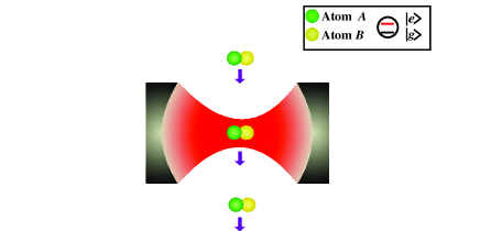
Figure 1: (Color online). Schematic diagram of the dynamic model of a series of TLAPs initially prepared in a general X-state randomly passing through a single-mode cavity. The two-level atoms in each TLAP respectively denoted as $A$ (the left green solid ball) and $B$ (the right yellow one). When the TLAPs pass through the cavity the coherence information in the TLAPs will transfer into the cavity.

We suppose that the pairwise TLAPs are randomly sent through the cavity for a fixed time interval $\tau$ and there is at most one TLAP in the cavity each time, and then the dynamic evolution of the whole system (cavity + TLAP) during each time interval is a unitary evolution and governed by the interaction Hamiltonian, $\hat{H}_{int}$. The unitary evolution operator in the interaction picture reads as

$$\hat{U}(\tau)\equiv\exp(-i\hat{H}_{int}\tau)=\left({\begin{array}[]{*{20}c}{\hat{U}_{11}}&{\hat{U}_{12}}&{\hat{U}_{13}}&{\hat{U}_{14}}\\ {\hat{U}_{21}}&{\hat{U}_{22}}&{\hat{U}_{23}}&{\hat{U}_{24}}\\ {\hat{U}_{31}}&{\hat{U}_{32}}&{\hat{U}_{33}}&{\hat{U}_{34}}\\ {\hat{U}_{41}}&{\hat{U}_{42}}&{\hat{U}_{43}}&{\hat{U}_{44}}\end{array}}\right),$$ (6)

where the matrix elements are expressed as

$$\hat{U}_{11}= 1+2\hat{a}\frac{{\hat{A}-1}}{\hat{\Lambda}}\hat{a}^{{\dagger}},~{}~{}~{}~{}~{}\hat{U}_{44}=1+2\hat{a}^{{\dagger}}\frac{{\hat{A}-1}}{\hat{\Lambda}}\hat{a},$$

$$\hat{U}_{22}= \hat{U}_{33}=\frac{1}{2}({\hat{A}+1}),~{}~{}~{}~{}\hat{U}_{23}=\hat{U}_{32}=\frac{1}{2}({\hat{A}-1}),$$

$$\hat{U}_{14}= 2\hat{a}\frac{{\hat{A}-1}}{\hat{\Lambda}}\hat{a},~{}~{}~{}~{}~{}~{}~{}~{}~{}~{}~{}~{}~{}\hat{U}_{41}=2\hat{a}^{{\dagger}}\frac{{\hat{A}-1}}{\hat{\Lambda}}\hat{a}^{{\dagger}},$$

$$\hat{U}_{12}= \hat{U}_{13}=-i\hat{a}\frac{{\hat{B}}}{{\sqrt{\hat{\Lambda}}}},~{}~{}~{}~{}~{}\hat{U}_{21}=\hat{U}_{31}=-i\frac{{\hat{B}}}{{\sqrt{\hat{\Lambda}}}}\hat{a}^{{\dagger}}\hfill,$$

$$\hat{U}_{42}= \hat{U}_{43}=-i\hat{a}^{{\dagger}}\frac{{\hat{B}}}{{\sqrt{\hat{\Lambda}}}},~{}~{}~{}\hat{U}_{24}=\hat{U}_{34}=-i\frac{{\hat{B}}}{{\sqrt{\hat{\Lambda}}}}\hat{a},\hfill$$

and

$$\hat{\Lambda}=2({2\hat{a}^{{\dagger}}\hat{a}}+1),~{}~{}\xi=g\tau,{}{} \hat{A}=\cos(\xi\sqrt{\hat{\Lambda}}), \hat{B}=\sin(\xi\sqrt{\hat{\Lambda}}).$$

We assume that the $j$th TLAP is injected into the cavity at time $t_{j}$, then, after a time interval $\tau$, the density matrix of the cavity field becomes

$$\hat{\rho}_{ca}(t_{j}+\tau)=\texttt{Tr}_{\textrm{AB}}[\hat{U}(\tau)\hat{\rho}_{\textrm{AB}}\otimes\hat{\rho}_{ca}(t_{j})\hat{U}^{\dagger}\left(\tau\right)]\equiv\mathcal{D}(\tau)\hat{\rho}_{ca}(t_{j}),$$ (7)

where $\hat{\rho}_{\textrm{AB}}$ is the density matrix of the $j$th TLAP and $\mathcal{D}(\tau)$ is a superoperator.

Since the TLAPs pass through the cavity randomly we assume that each one arrives at the cavity with a probability $r$ per unit time. The probability of a TLAP arrival, in a time interval of $(t,t+\delta t)$, is $r\delta t$, and the probability without the TLAP passing is $1-r\delta t$. Hereafter, for simplicity, we denote $\hat{\rho}_{ca}$ as $\hat{\rho}$. Then we can obtain the density matrix of cavity field at time $t+\delta t$  Sun

$$\hat{\rho}(t+\delta t)=(1-r\delta t)\hat{\rho}(t)+r\delta t\mathcal{D}(\tau)\hat{\rho}(t).$$ (8)

For $\delta t\rightarrow 0$, one obtains the master equation Scully3 ; Orszag ; Meschede ; Casagrande ; Cresser ; Cresser96 ; Bergou ; Guerra

$$\dot{\hat{\rho}}(t)=r[\mathcal{D}(\tau)-1]\hat{\rho}(t),$$ (9)

which describes the dynamics of the single-mode cavity field.

III dynamics of cavity field with a nonequilibrium reservoir

Here, we consider a nonequilibrium reservoir consisting of a beam of TLAPs in a general X-state, and in the basis $\{|ee\rangle,|eg\rangle,|ge\rangle,|gg\rangle\}$, the X-state is given by

$$\hat{\rho}_{AB}=\left({\begin{array}[]{*{20}c}{{a}_{11}}&0&0&{{a}_{14}}\\ 0&{{a}_{22}}&{{a}_{23}}&0\\ 0&{{a}_{32}}&{{a}_{33}}&0\\ {{a}_{41}}&0&0&{{a}_{44}}\end{array}}\right),$$ (14)

where $\hat{\rho}_{AB}$ is normalized $\sum_{i=1}^{4}{a}_{ii}=1$, and the nondiagonal elements ${a}_{14}={a}_{41}^{*}$ and ${a}_{23}={a}_{32}^{*}$. Inserting Eq. (14) into Eq. (7) and after some calculations, the superoperator $\mathcal{D}(\tau)$ can be expressed as

$$\mathcal{D}(\tau)\hat{\rho}(t)=\sum_{i,j=1}^{4}{a}_{ij}\sum_{m=1}^{4}\hat{U}_{mi}(\tau)\hat{\rho}(t)\hat{U}_{mj}^{\dagger}(\tau),$$ (15)

where ${a}_{ij}$ $(i,j=1,2,3,4)$ are given in Eq. (14). Thus, for the X-state one has

$$\hat{\rho}(t_{j}+\tau)=\sum_{i,j=1}^{4}{a}_{ij}\sum_{m=1}^{4}\hat{U}_{mi}(\tau)\hat{\rho}(t)\hat{U}_{mj}^{\dagger}(\tau)$$ (16)

describing the density matrix of the cavity field at time $t_{j}+\tau$, and the master equation Eq. (9) can be rewritten as

$$\dot{\hat{\rho}}(t)=r[\sum_{i,j=1}^{4}{a}_{ij}\sum_{m=1}^{4}\hat{U}_{mi}(\tau)\hat{\rho}(t)\hat{U}_{mj}^{\dagger}(\tau)-\hat{\rho}(t)].$$ (17)

Eq (17) is the quantum master equation of the cavity field for each TLAP in the X-state. In order to obtain the dynamics of the cavity field we consider two cases of the TLAPs passing through the cavity: ${1)}$ passing through instantly corresponding to $\xi\rightarrow 0$, and ${2)}$ passing through at a low speed corresponding to a finite $\xi$. In case 1, Eqs. (16) and (17) can be further expressed as

$$\hat{\rho}({t_{j}+\tau})\approx \xi^{2}\{{{({2a_{11}+a_{22}+a_{33}+a_{23}+a_{32}})[{\hat{a}^{\dagger}\hat{\rho}({t_{j}})\hat{a}-\hat{\rho}({t_{j}})}]}}$$ (18)

$$+ ({2a_{44}+a_{22}+a_{33}+a_{23}+a_{32}})\hat{a}\hat{\rho}({t_{j}})\hat{a}^{\dagger}$$

$$- ({a_{11}+a_{44}+a_{23}+a_{32}})\hat{a}^{\dagger}\hat{a}\hat{\rho}({t_{j}})$$

$$- ({1+a_{22}+a_{33}+a_{23}+a_{32}})\hat{\rho}({t_{j}})\hat{a}^{\dagger}\hat{a}$$

$$+ a_{14}(2\hat{a}^{{\dagger}}\hat{\rho}\hat{a}^{{\dagger}}-\hat{a}^{{\dagger}}\hat{a}^{{\dagger}}\hat{\rho}-\hat{\rho}\hat{a}^{{\dagger}}\hat{a}^{{\dagger}})$$

$$+ a_{41}(2\hat{a}\hat{\rho}\hat{a}-\hat{a}\hat{a}\hat{\rho}-\hat{\rho}\hat{a}\hat{a})\}+\hat{\rho}({t_{j}})$$

and

$$\dot{\hat{\rho}}\approx r\xi^{2}\{a_{11}(2\hat{a}^{{\dagger}}\hat{\rho}\hat{a}-\hat{\rho}\hat{a}\hat{a}^{{\dagger}}-\hat{a}\hat{a}^{{\dagger}}\hat{\rho})$$ (19)

$$+ {a_{44}(2\hat{a}\hat{\rho}\hat{a}^{{\dagger}}-\hat{\rho}\hat{a}^{{\dagger}}\hat{a}-\hat{a}^{{\dagger}}\hat{a}\hat{\rho})}$$

$$- (a_{22}+a_{33})[(2\hat{\rho}\hat{a}^{{\dagger}}\hat{a}-\hat{a}\hat{\rho}\hat{a}^{{\dagger}}-\hat{a}^{{\dagger}}\hat{\rho}\hat{a})+\hat{\rho}]$$

$$+ a_{14}(2\hat{a}^{{\dagger}}\hat{\rho}\hat{a}^{{\dagger}}-\hat{a}^{{\dagger}}\hat{a}^{{\dagger}}\hat{\rho}-\hat{\rho}\hat{a}^{{\dagger}}\hat{a}^{{\dagger}})$$

$$+ a_{41}(2\hat{a}\hat{\rho}\hat{a}-\hat{a}\hat{a}\hat{\rho}-\hat{\rho}\hat{a}\hat{a})$$

$$+ (a_{23}+a_{32})(\hat{a}\hat{\rho}\hat{a}^{{\dagger}}+\hat{a}^{{\dagger}}\hat{\rho}\hat{a}-\hat{a}^{{\dagger}}\hat{a}\hat{\rho}-\hat{\rho}\hat{a}^{{\dagger}}\hat{a}-\hat{\rho})\},$$

where we have made the approximation $\hat{A}=\cos(\xi\sqrt{{\hat{\Lambda}}})\approx 1-\xi^{2}{\hat{\Lambda}}/2$ and $\hat{B}=\sin(\xi\sqrt{{\hat{\Lambda}}})\approx\xi\sqrt{{\hat{\Lambda}}}$, and kept $\xi$ up to the second order. For simplicity, we denote $\hat{\rho(t)}$ in Eq. (19) as $\hat{\rho}$. In case 2, the above approximation is not valid any more and from Eq. (16) the density matrix of cavity field at time $t_{j}+\tau$ can be rewritten as

$$\hat{\rho}(t_{j}+\tau)= \sum_{m,n=0}^{\infty}\{\rho_{m,n}f_{1}+\rho_{m+1,n+1}f_{2}+\rho_{m-1,n-1}f_{3}$$ (20)

$$+ \rho_{m-2,n-2}f_{4}+\rho_{m+2,n+2}f_{5}+\rho_{m,n+2}f_{6}$$

$$+ \rho_{m+2,n}f_{7}+\rho_{m+1,n-1}f_{8}+\rho_{m-1,n+1}f_{9}$$

$$+ \rho_{m,n-2}f_{10}+\rho_{m-2,n}f_{11}\}|m\rangle\langle n|,$$

where $\rho_{m,-2}=\rho_{m,-1}=\rho_{-2,n}=\rho_{-1,n}=0$, $(m,n=0,1,2,...)$, and during the derivation we have assumed that the state of cavity field $\hat{\rho}(t_{j})=\sum_{m,n=0}^{\infty}\rho_{m,n}(t_{j})|m\rangle\langle n|$ and denoted $\rho_{m,n}(t_{j})$ as $\rho_{m,n}$. For simplicity, $f_{i}$ ($i=1,2,3,...,11$) are given in the appendix A. Though the expression of Eq. (20) is complex, it, in the limit $\xi\rightarrow 0$, is in consistency with Eq. (18).

Next, we first consider the dynamics of the cavity field in case 1. For simplicity, throughout this paper we choose the vacuum state as the initial state of the cavity field. From Eq. (18) it can be seen that the density matrices $\hat{\rho}(t_{j}+\tau)$ and $\hat{\rho}(t_{j})$ possess the same form of structure. When considering the cavity initially prepared in vacuum state (being in the diagonal distribution), the density matrix of cavity field, $\hat{\rho}(t_{j}+\tau)$, will keep the diagonal distribution. Moreover, from Eq. (18) we can obtain that the average photon number of the cavity field at time ${t_{j}+\tau}$ reads as

$$\langle\hat{n}(t_{j}+\tau)\rangle= \texttt{Tr}[{\hat{\rho}}(t_{j}+\tau)\hat{n}]$$ (21)

$$= [2\xi^{2}(a_{11}-a_{44})+1]\langle\hat{n}(t_{j})\rangle$$

$$+ \xi^{2}(2a_{11}+a_{22}+a_{33}+a_{23}+a_{32}).$$

From Eq. (21) it can be seen that the increment of average photon number between two neighboring passings $\Delta\langle\hat{n}(t_{j}+\tau)\rangle=\langle\hat{n}(t_{j}+\tau)\rangle-\langle\hat{n}(t_{j})\rangle$, satisfies

$$\Delta\langle\hat{n}(t_{j}+\tau)\rangle=[1-2\xi^{2}(a_{44}-a_{11})]\Delta\langle\hat{n}(t_{j})\rangle.$$ (22)

The increment ratio, $k$, for the two neighboring passings at time $t_{j}$ and $t_{j}+\tau$ is directly obtained as

$$k=\frac{\Delta\langle\hat{n}(t_{j}+\tau)\rangle}{\Delta\langle\hat{n}(t_{j})\rangle}=1-2\xi^{2}(a_{44}-a_{11}).$$ (23)

Since the initial state of the cavity field is supposed to be the vacuum state, i.e., $\langle\hat{n}(0)\rangle=0$, from Eq. (21) the average photon number after the first passing is

$$\langle\hat{n}(\tau)\rangle=\xi^{2}(2a_{11}+a_{22}+a_{33}+a_{23}+a_{32}).$$ (24)

From Eqs. (23) and (24) the average photon number, after the $j$th time passing (i.e., at time $t_{j}$), can be expressed as

$$\langle\hat{n}(t_{j})\rangle=\sum_{i=1}^{j}k^{i-1}\langle\hat{n}(\tau)\rangle.$$ (25)

According to Eqs. (23) and (25) for $a_{11}\geq a_{44}$ the ratio $k\geq 1$ holds which means that the average photon number, $\langle\hat{n}(t_{j})\rangle$, is divergent. On the contrary, for $k<1$ $(a_{11}<a_{44})$, $\langle\hat{n}(t_{j})\rangle$ is convergent, and in the limit $j\rightarrow\infty$ (i.e., $t_{j}\rightarrow\infty$)

$$\langle\hat{n}(t_{j})\rangle|_{j\rightarrow\infty}=\frac{\langle\hat{n}(\tau)\rangle}{1-k}=\frac{{2a_{11}+a_{22}+a_{33}+a_{23}+{a}_{32}}}{{2\left({a_{44}-a_{11}}\right)}}.$$ (26)

Eq. (26) shows that for fixed X-state with $a_{11}<a_{44}$ the cavity field, in the limit $t_{j}\rightarrow\infty$, can reach a steady state. Besides, this result can also be verified by the master equation Eq. (19) from which, after some calculations, we have

$$\langle\dot{\hat{n}}\rangle=r\xi^{2}\left[{2\left({a_{11}-a_{44}}\right)\left\langle{\hat{n}}\right\rangle+2a_{11}+a_{22}+a_{33}+a_{23}+a_{32}}\right]=0,$$ (27)

and

$$\left\langle{{\hat{n}}}\right\rangle_{ss}=\frac{{2a_{11}+a_{22}+a_{33}+a_{23}+{a}_{32}}}{{2\left({a_{44}-a_{11}}\right)}},$$ (28)

where $\langle\hat{n}\rangle_{ss}=\langle\hat{n}(t_{j}\rightarrow\infty)\rangle$ represents the average photon number of the cavity in the steady state.

Here, we consider two special noncoherent states of TLAPs, $\hat{\rho}_{AB}^{(1)}$ with classical correlation and $\hat{\rho}_{AB}^{(2)}$ without any correlation (i.e., product state), as follows

$${\hat{\rho}_{AB}^{(1)}}= a_{11}|ee\rangle\langle ee|+a_{22}|eg\rangle\langle eg|+a_{33}|ge\rangle\langle ge|+a_{44}|gg\rangle\langle gg|,$$ (29)

and

$${\hat{\rho}_{AB}^{(2)}}=\hat{\rho}_{A}\otimes\hat{\rho}_{B},$$ (30)

where $\hat{\rho}_{A}$ and $\hat{\rho}_{B}$ respectively read as

$$\hat{\rho}_{A}=\left({\begin{array}[]{*{20}c}{a}_{11}+{a}_{22}&0\\ 0&{a}_{33}+{a}_{44}\end{array}}\right)$$ (33a)

$$\hat{\rho}_{B}=\left({\begin{array}[]{*{20}c}{a}_{11}+{a}_{33}&0\\ 0&{a}_{22}+{a}_{44}\end{array}}\right).$$ (35b)

It is noted that the choice of above two states enables the three density matrices $\hat{\rho}_{AB}$ and $\hat{\rho}_{AB}^{(m)}$ (${m=1,2}$) to possess the same reduced density matrices $\hat{\rho}_{A}$ and $\hat{\rho}_{B}$. In terms of Eq. (28) when the TLAPs are initially prepared in the states $\hat{\rho}_{AB}^{(1)}$ and $\hat{\rho}_{AB}^{(2)}$, respectively, one has

$$\langle\hat{n}\rangle_{ss}^{(m)}=\frac{{2a_{11}+a_{22}+a_{33}}}{{2\left({a_{44}-a_{11}}\right)}},$$ (36)

where $\langle\hat{n}\rangle_{ss}^{(m)}$ represents the average photon number of the cavity in the steady state for $\hat{\rho}_{AB}^{(m)}$ (${m=1,2}$).

Especially, if we consider $\hat{\rho}_{A}=\hat{\rho}_{B}$ (i.e., $a_{22}=a_{33}$) and $a_{11}+a_{22}<a_{33}+a_{44}$ the temperature of reservoir consisting of TLAPs can be defined well by the two-level atoms. For simplicity, we denote ${p}_{e}=a_{11}+a_{22}$ and ${p}_{g}=a_{22}+a_{44}$ the inverse temperature of reservoir $\beta_{\textrm{eff}}$ ($\beta_{\textrm{eff}}=1/(k_{B}T)$, $k_{B}$ is the Boltzmann constant) is expressed as

$$\frac{p_{e}}{p_{g}}=e^{-\beta_{\textrm{eff}}\omega}\Rightarrow\beta_{\textrm{eff}}=-\frac{1}{\omega}\ln\frac{p_{e}}{p_{g}},$$ (37)

where we let $\hbar=1$. In this case, the asymptotic solution of the master equation Eq. (19) is the thermal state. From Eqs. (28) and (36) the thermal average photon numbers $\langle\hat{n}\rangle_{th}=\frac{a_{11}+a_{22}+\texttt{Re}[a_{23}]}{a_{44}-a_{11}}$ for ${\hat{\rho}_{AB}}$ corresponds to the inverse temperatures of cavity field

$${\beta}_{coh}=-\frac{1}{\omega}\ln\frac{\langle\hat{n}\rangle_{th}}{1+\langle\hat{n}\rangle_{th}}=-\frac{1}{\omega}\ln\frac{p_{e}+\texttt{Re}[a_{23}]}{p_{g}+\texttt{Re}[a_{23}]},$$ (38)

and $\langle\hat{n}\rangle_{th}^{(m)}=\frac{a_{11}+a_{22}}{a_{44}-a_{11}}$ for $\hat{\rho}_{AB}^{(m)}$ (m=1,2) with

$${\beta}_{non}^{(m)}=-\frac{1}{\omega}\ln\frac{\langle\hat{n}\rangle_{th}^{(m)}}{1+\langle\hat{n}\rangle_{th}^{(m)}}=-\frac{1}{\omega}\ln\frac{p_{e}}{p_{g}}.$$ (39)

From Eqs. (37-39) we can see that for the noncoherent reservoir with ${\hat{\rho}_{AB}^{(m)}}$ the cavity field is thermalized and reaches the same temperature as the reservoir, ${\beta}_{non}^{(m)}=\beta_{\textrm{eff}}$, but for the coherent reservoir with ${\hat{\rho}_{AB}}$ the temperature of cavity field after thermalization does not coincide with the reservoir’s any more due to the reservoir’s coherence, i.e., ${\beta}_{coh}\neq\beta_{\textrm{eff}}$. It is similar to the model of a single atom coherent reservoir in Ref. Scully where Scully et al. showed that the detailed balance between photon absorption and emission could be broken with the help of the coherent superposition of the two (nearly degenerate) lower levels of a three-level atom. In our model, the TLAP has four energy levels including a higher level with double excitation $|ee\rangle$, a lower level with no excitation $|gg\rangle$ and two degenerate intermediate levels respectively corresponding to single excitation $|eg\rangle$ and $|ge\rangle$. Here, we can also use the coherent superposition of the two degenerate intermediate levels of the TLAP to break the detailed balance. Meanwhile, the deviation away from thermal equilibrium is completely determined by the real part of the coherence term (see Eq. (38)), i.e., $\texttt{Re}[a_{23}]=|a_{23}|\cos\phi$ where we denote $\phi$ as the relative phase between the two degenerate intermediate levels in the TLAP. It is clear that the reservoir’s coherence in our model also plays an important role in the thermalization of the cavity field.

In addition, from Eq. (36) it can be seen that the cavity field possesses the same average photon number for $\hat{\rho}_{AB}^{(1)}$ and $\hat{\rho}_{AB}^{(2)}$ which implies that the classical correlation of the TLAP has no contribution to the work capability of cavity field. Actually, even for the quantum correlations including the QE and QD they are not always good quantities to effectively reflect the contributions of the TLAPs to the work capability of cavity field. Using the density matrix Eq. (14), the quantum correlations between the two atoms in each TLAP as measured by QE and QD can be calculated. We adopt Wootter’s concurrence Wootters as entanglement measure. For the density matrix Eq. (14), the concurrence is given by

$$C(\hat{\rho}_{AB})=2\max(0,|a_{23}|-\sqrt{a_{11}a_{44}},|a_{14}|-\sqrt{a_{22}a_{33}}).$$ (40)

On the other hand, quantum discord captures all nonclassical correlations between two two-level atoms Ollivier . For the X state described by the density matrix Eq. (14), the analytic expression of QD has been reported Wang and expressed by

$${Q}(\hat{\rho}_{AB})=\min({Q_{1}},{Q_{2}}),$$ (41)

where $Q_{j}=H(a_{11}+a_{33})+\sum_{i=1}^{4}\lambda_{i}\log_{2}\lambda_{i}+D_{j}$ with $\lambda_{i}$ being the four eigenvalues of $\hat{\rho}_{AB}$, $D_{1}(\tau)=H(\tau)$, $D_{2}(\tau)=-\sum_{i=1}^{4}a_{ii}\log_{2}a_{ii}-H(a_{11}+a_{33})$ with $\tau=(1+\sqrt{[1-2(a_{33}+a_{44})]^{2}+4(|a_{14}|+|a_{23}|)^{2}})/{2}$ and $H(\tau)=-\tau\log_{2}\tau-(1-\tau)\log_{2}(1-\tau)$. For the convenience of discussion we give our construction of the general X-state. As we know, the space of a general X-state is composed of two independent subspaces which are spanned by the base vectors $\{|ee\rangle,|gg\rangle\}$ and $\{|eg\rangle,|ge\rangle\}$, respectively. We can choose the arbitrary state in each subspace to construct the X-state via the direct sum as follows

$$\hat{\rho}_{AB}= \cos^{2}\alpha\hat{\rho}_{1}^{\prime}\oplus\sin^{2}\alpha\hat{\rho}_{2}^{\prime}= \left({\begin{array}[]{*{20}c}{\frac{1}{2}{\cos^{2}\alpha}(1+{r}_{1}\cos\theta_{1})}&0&0&{\frac{1}{2}r_{1}{\cos^{2}\alpha}\sin\theta_{1}e^{-i\varphi}}\\ 0&{\frac{1}{2}{\sin^{2}\alpha}(1+{r}_{2}\cos\theta_{2})}&{\frac{1}{2}r_{2}{\sin^{2}\alpha}\sin\theta_{2}e^{-i\phi}}&0\\ 0&{\frac{1}{2}r_{2}{\sin^{2}\alpha}\sin\theta_{2}e^{i\phi}}&{\frac{1}{2}{\sin^{2}\alpha}(1-{r}_{2}\cos\theta_{2})}&0\\ {\frac{1}{2}r_{1}{\cos^{2}\alpha}\sin\theta_{1}e^{i\varphi}}&0&0&{\frac{1}{2}{\cos^{2}\alpha}(1-r_{1}\cos\theta_{1})}\end{array}}\right),$$ (46)

in which the density matrices $\hat{\rho}_{1,2}^{\prime}=\frac{1}{2}(\mathbb{I}_{1,2}+\vec{r}_{1,2}\cdot\vec{\sigma}_{1,2})$, respectively, represent the arbitrary state in each subspace where $\mathbb{I}_{1}(\mathbb{I}_{2})$ is a unit matrix in the state space of $\hat{\rho}_{1}^{\prime}(\hat{\rho}_{2}^{\prime})$, $\vec{r}_{1,2}$ are the Bloch sphere vectors, and $\vec{\sigma}_{1,2}$ are the pauli matrices with $\hat{\sigma}_{1z}=|ee\rangle\langle ee|-|gg\rangle\langle gg|$ and $\hat{\sigma}_{2z}=|eg\rangle\langle eg|-|ge\rangle\langle ge|$. And we assume that the probability of the TLAP in each subspace is respectively $\cos^{2}\alpha$ $(\sin^{2}\alpha)$. The parameters in the X-state of Eq. (46) satisfy $\alpha\in[0,\pi/2]$, $\theta_{1},\theta_{2}\in[0,\pi]$, $\varphi,\phi\in[0,2\pi]$ and $r_{1},r_{2}\in[0,1]$ which guarantee the positivity, normalization and trace preservation of $\hat{\rho}_{AB}$. By choosing proper parameters of the X-state in Eq. (46) we can find some states which only possess coherence but no quantum correlations. That is, these states have nondiagonal elements but their concurrence (quantum entanglement) and quantum discord are zero. As an example, we choose the parameters: $r_{1}=r_{2}=2/3$, $\alpha=\sqrt{\pi}/4$, $\theta_{1}=\theta_{2}=11\pi/20$, $\varphi=\pi/3$, $\phi_{2}=0$, and the X-state becomes

$$\hat{\rho}_{1}=\left({\begin{array}[]{*{20}c}{0.223928}&0&0&{0.0823074-0.142561i}\\ 0&{0.223928}&{0.164615}&0\\ 0&{0.164615}&{0.276072}&0\\ {0.0823074+0.142561i}&0&0&{0.276072}\end{array}}\right).$$ (51)

From Eqs. (40) and (41) we can obtain that $C(\hat{\rho}_{1})=Q(\hat{\rho}_{1})=0$. It is noted that although the state $\hat{\rho}^{\texttt{dia}}_{1}$, only preserving the diagonal elements of density matrix in Eq. (51), has no quantum correlations like $\hat{\rho}_{1}$ the average photon numbers of cavity field in the two cases are different. This mean that quantum coherence can be the work resource even in the absence of quantum correlations.

Meanwhile, although the states of the TLAPs, $\hat{\rho}_{AB}$ and $\hat{\rho}_{AB}^{(m)}$ (m=1,2) have the same reduced density matrices as mentioned before, they lead to different average photon numbers of cavity field $\langle\hat{n}\rangle_{ss}$ and $\langle\hat{n}\rangle_{ss}^{(m)}$ given in Eqs. (28) and (36), respectively. It is noted that from Eqs. (28) and (36) $\langle\hat{n}\rangle_{ss}\geq\langle\hat{n}\rangle_{ss}^{(m)}$ for $a_{23}+a_{32}\geq 0$; $\langle\hat{n}\rangle_{ss}<\langle\hat{n}\rangle_{ss}^{(m)}$ for $a_{23}+a_{32}<0$. So, it means that due to the coherence of the TLAPs not only the constructive quantum interference but also the destructive quantum interference can be induced and cause the average photon number of cavity field away from $\langle\hat{n}\rangle_{ss}^{(m)}$ corresponding to $\hat{\rho}_{AB}^{(m)}$ (m=1,2) without any coherence. This is an interesting and meaningful thing, and by using it we can easily perform a thermodynamic cycle with a single nonequilibrium reservoir only by controlling an external parameter, i.e., the relative phase. Furthermore, in terms of the definitions of quantum correlations in Eqs. (40) and (41), QE and QD are only related to the amplitude of the nondiagonal terms in the X-state and independent of the relative phase. It demonstrates that quantum correlations could not always reflect the effects of reservoir on the system’s work capability completely, and the relative phase of the TLAP also plays an important role.

Moreover, we also notice that Dillenschneider et al. in Ref. Lutz also considered the same model where a series of TLAPs pass through a cavity. They showed that the quantum correlations act as the resource of system’s work capability which seems to be contradictory with our results (the reservoir’s coherence acting as the resource rather than the quantum correlations). In fact, it is not that case. This can be explained as follows. The state of TLAP considered in Ref. Lutz is a thermal entangled state which belongs to a very special X-state with $a_{22}=a_{33}$, $a_{14}=a_{41}=0$ and $a_{23}=a_{32}=-|a_{23}|$. For this state we can obtain the average photon number of the cavity field in the final steady state as

$$\langle\hat{n}_{1}\rangle_{ss}=\frac{a_{11}+a_{22}-|a_{23}|}{a_{44}-a_{11}}=\langle\hat{n}\rangle_{det}+\Delta,$$ (52)

where $\langle\hat{n}\rangle_{det}=\frac{a_{11}+a_{22}}{a_{44}-a_{11}}$ represents the average photon number for the system being in the detailed balance, and $\Delta=-\frac{|a_{23}|}{a_{44}-a_{11}}$ denotes the deviation from the detailed balance. Since $|a_{23}|$ can effectively reflect the quantum correlations of the thermal entangled X-state the deviation term, $\Delta$, can not only be understood as the thermodynamic effects of quantum coherence on cavity field but also the contribution of quantum correlations. In order to demonstrate that quantum correlations are not good physical quantities to effectively reflect the thermodynamic effects of nonequilibrium reservoir, we could implement a quantum phase gate operation on one of the atoms in the TLAP to make the coherence term $a_{23}$ $(a_{32})$ of the thermal entangled state add a relative phase factor, i.e., the transition $a_{23}$ $(a_{32})\rightarrow e^{-i\phi}a_{23}$ $(e^{i\phi}a_{32})=-e^{-i\phi}|a_{23}|$ $(-e^{i\phi}|a_{32}|)$, $\phi\in[0,\pi]$. It is noted that this operation only adds a relative phase and does not change the quantum correlations (concurrence and QD) of the TLAP. For the state after the operation the average photon number of the cavity field in the steady state can be expressed as

$$\langle\hat{n}_{2}\rangle_{ss}=\langle\hat{n}\rangle_{det}+\Delta\cos\phi.$$ (53)

From Eq. (53) it is clear that, for the average photon number of the cavity field, the deviation from the detailed balance not only depends on the quantum correlations but also on the relative phase, and via modifying the relative phase the instructive and the destructive interferences could be introduced. Comparing Eqs. (52) and (53) we can see that even though the TLAPs have the same quantum correlations they could correspond to different average photon number, i.e., $\langle\hat{n}_{1}\rangle_{ss}\neq\langle\hat{n}_{2}\rangle_{ss}$ for $\phi\neq 0$. This demonstrates that, in general, the reservoir’s quantum correlations could not completely reflect the influence of a nonequilibrium reservoir on the work capability of the cavity field, and the relative phase also plays an important role. And by modifying the relative phase the deviation from the detailed balance for the average photon number may be positive, negative or zero.

From Eq. (28) we can see that the coherence elements $a_{14}$ and $a_{41}$ do not like $a_{23}$ and $a_{32}$ contribute to the average photon number $\langle\hat{n}\rangle_{ss}$. They seem to have no effect on the average photon number. In fact, it is not that case. This can be explained that $a_{14}$ ($a_{41}$) corresponds to the process of the double excitation during the evolution of the cavity field, and appears in the higher order terms than the second order term $\xi^{2}$ of the average photon number. In the limit $\xi\rightarrow 0$, these high order terms can be omitted, however, they can not be ignored any more in case 2 with finite $\xi$. In case 2 the effects of coherence $a_{14}$ $(a_{41})$ on the dynamics of the cavity field will be fully demonstrated.

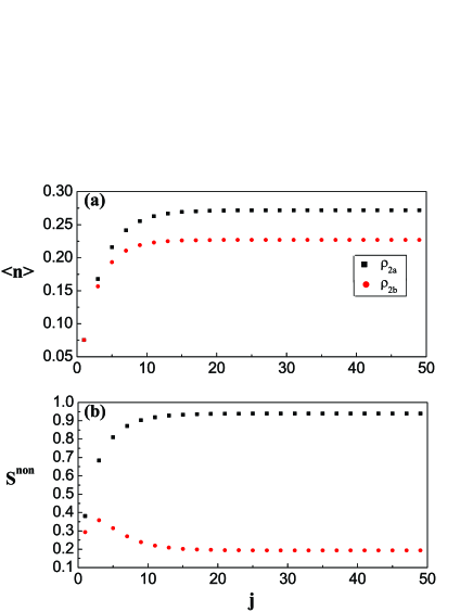
Figure 2: (Color online). (a) The variations of the average photon number, $\langle\hat{n}\rangle$, and (b) the variations of the entropy, $S^{non}$, of the cavity field with passing times, $j$, for state $\hat{\rho}_{2a}$ (black squares) and $\hat{\rho}_{2b}$ (red dots).

From Eq. (20) we can see that the expression of the density matrix of the cavity after the $(j+1)$th passing of the TLAPs is very complicated, and the nondiagonal elements appear in the density matrix which is very different from that in case 1. Thus, it is very difficult to obtain general analytical expressions of the average photon number and the entropy of the cavity field during the evolution. Next, we will make use of numerical calculations to explore the dynamics of the cavity field. In order to demonstrate the effects of coherence terms $a_{14}$ and $a_{41}$ in the X-state given in Eq. (14) we consider the TLAPs being respectively prepared in the following two states

$$\hat{\rho}_{2a}=\left({\begin{array}[]{*{20}c}{0.142864}&0&0&{0}\\ 0&{0.0122355}&{0.0012236}&0\\ 0&{0.0012236}&{0.0122355}&0\\ {0}&0&0&{0.832665}\end{array}}\right)$$ (58)

and

$$\hat{\rho}_{2b}=\left({\begin{array}[]{*{20}c}{0.142864}&0&0&{0.344901}\\ 0&{0.0122355}&{0.0012236}&0\\ 0&{0.0012236}&{0.0122355}&0\\ {0.344901}&0&0&{0.832665}\end{array}}\right),$$ (63)

where from Eq. (46) we choose the parameters $\{r_{1}=0.7071,r_{2}=0.1,\alpha=\pi/20,\theta_{1}=\pi,\theta_{2}=\pi/2,\varphi=\phi=0\}$ for $\hat{\rho}_{2a}$ and $\{r_{1}=1,r_{2}=0.1,\alpha=\pi/20,\theta_{1}=3\pi/4,\theta_{2}=\pi/2,\varphi=\phi=0\}$ for $\hat{\rho}_{2b}$. It is noted that $a_{14}=0$ in $\hat{\rho}_{2a}$ and $a_{14}=0.344901$ in $\hat{\rho}_{2b}$ and the other density matrix elements are the same. Hereafter, we set $\xi=0.5$. In terms of Eq. (20) we plot the variations of the average photon number, $\langle\hat{n}\rangle$, and the entropy, $S^{non}$, of the cavity field with passing times, $j$, for $\hat{\rho}_{2a}$ and $\hat{\rho}_{2b}$ in Fig. 2. Throughout this paper, the entropy of the cavity field is defined by von Neumann entropy $S(\rho)=-k_{B}\texttt{Tr}(\rho\log_{2}\rho)$, and for simplicity, we set $k_{B}=1$. From Fig. 2 it can be seen that the nondiagonal element $a_{14}$ ($a_{41}$) has an obvious effects on the average photon number shown in Fig. 2(a) and the entropy of the cavity field in Fig. 2(b), and the values of $\langle\hat{n}\rangle$ and $S^{non}$, for $\hat{\rho}_{2a}$ are always larger than those for $\hat{\rho}_{2b}$. Moreover, we also see that the changes of the entropy and the average photon number of cavity field are obvious for the first few passings and for $j>10$ the entropy and the average photon number gradually approach their steady values, respectively.

On the other hand, $\xi$ could also affect the dynamic behavior of the cavity field, such as the average photon number and the entropy. Different from case 1 $\xi\rightarrow 0$ $(\xi=g\tau)$ the cavity field could exhibit very different and complicated dynamic behaviors in case 2 with finite $\xi$ even though we choose the same nonequilibrium reservoir. The finite $\xi$ could be understood as a strong coupling or a long interaction time interval between the TLAP and the cavity field, and in this case the double excitation process corresponding to the coherent term $a_{14}$ $(a_{41})$ is involved in the dynamic evolution of the cavity field in case 2, while for $\xi\rightarrow 0$ in case 1 this can not occur. According to the unitary operator $\hat{U}(\tau)$ in Eq. (6) we can see that each element of $\hat{U}(\tau)$ in case 2 is a nonlinear function of $\xi$ that could lead to a very complicated evolution of the cavity field, $\hat{\rho}(t_{j}+\tau)$ in Eq. (20). From the density matrix $\hat{\rho}(t_{j}+\tau)$ it can be seen that the single excitation process corresponding to the coherent term $a_{23}$ $(a_{32})$, the double excitation process with coherence $a_{14}$ $(a_{41})$ and the parameter $\xi$ are all involved in the cavity evolution in a very complicated way. Naturally, from the definitions of the average photon number and the entropy of the cavity field, we can infer that during the cavity evolution they are also closely related to the single excitation, double excitation processes, and the parameter $\xi$. Since the expressions of the average photon number and the entropy of the cavity field are very complicated we can only demonstrate how the parameter $\xi$ and reservoir’s coherence $a_{23}$ and $a_{14}$ influence the dynamics of the cavity by numerical calculations. Only as an example, we plot Fig. 2 to demonstrate the thermodynamic effects of the coherent term $a_{14}$ (or the double excitation process of the TLAP) on the dynamics of the cavity field for specific states of the TLAP $\hat{\rho}_{2a}$ and $\hat{\rho}_{2b}$, and $\xi$ ($\xi=0.5$). From a lot of numerical calculations we find that the dynamic behaviors of the cavity field are determined by $a_{23}$, $a_{14}$, and $\xi$ altogether. For example, suppose that the state of the TLAP is $\hat{\rho}_{AB}$ when we keep $\hat{\rho}_{AB}$ fixed and only change the value of $\xi$, or keep $\xi$ fixed and only change the values of the non-diagonal elements of $\hat{\rho}_{AB}$ the average photon number and the entropy of the cavity field usually could exhibit different variation curves with the passing times $j$, i.e., the entropy and the average photon number of the cavity field can exhibit monotonous behaviors for some specific $\xi$ and specific X-states of the TLAP, and non-monotonous behaviors for the others. For example, if we choose the state of the TLAP as $\hat{\rho}_{2b}$ given in Eq. (63) and $\xi=0.2$ instead of $\xi=0.5$ in Fig. 2 the entropy of the cavity will be monotonously increasing with $j$ which is very different from the non-monotonous behavior as shown in Fig. 2(b). Similarly, the monotonous increasing behavior of the entropy can also appear only by choosing the proper state of the TLAP and keeping $\xi$ unchanged such as $\xi=0.5$ and changing $\hat{\rho}_{2b}$ in Eq. (63) into the state $\hat{\tilde{\rho}}_{2b}$ with $\{r_{1}=0.7071,r_{2}=0.1,\alpha=\pi/4,\theta_{1}=3\pi/4,\theta_{2}=\pi/2,\varphi=\phi=0\}$ in Eq. (46). In Fig. 2(a) although the average photon number $\langle n\rangle$ exhibits a monotonous increasing behavior for $\hat{\rho}_{2b}$ and $\xi=0.5$ the curve of $\langle n\rangle$ can also exhibit the non-monotonous behavior for other value of $\xi$ and other state of the TLAP, such as $\xi=1.2$ and $\hat{\rho}_{AB}$ in Eq. (46) with $\{r_{1}=1,r_{2}=0.5,\alpha=\pi/20,\theta_{1}=3\pi/4,\theta_{2}=\pi/2,\varphi=\phi=0\}$. In addition, from numerical calculations we also find that if $a_{14}=0$ both the average photon number and the entropy of the cavity always monotonously increase with $j$ which indicates that the coherent term $a_{14}$ may effectively influence the dynamic behaviors of the cavity field in case 2 with finite $\xi$. This means that the non-monotonous behavior of the cavity field might be caused by the double excitation process corresponding to the coherent term $a_{14}$ for finite $\xi$.

Besides, for a cavity field coupled to a non-equilibrium atomic reservoir with effective temperature well defined by the two-level atom if the detailed balance is not broken the temperature of the cavity field being in a steady state will be the same as the effective temperature of the reservoir, and the cavity has the average photon number defined by the effective temperature of the reservoir. For the cavity field with the TLAPs being initially in the X-state $\hat{\rho}_{AB}$ in Eq. (14) if the detailed balance is not broken the average photon number of cavity field will only depend on the diagonal elements of $\hat{\rho}_{AB}$. In another word, if other parameters such as the coherence of the non-equilibrium reservoir, i.e., the non-diagonal elements of $\hat{\rho}_{AB}$, or the parameter $\xi$ enter into the average photon number of the cavity field the detailed balance in general could not be reached. From the density matrix of the cavity evolution $\hat{\rho}(t_{j}+\tau)$ in Eq. (20) we can see that the density matrix of the cavity field in case 2 always has nonzero nondiagonal elements which means that the cavity field always stays in a nonequilibrium state even if it reaches a steady state. In addition, we also notice that in case 2 all the coherence of the TLAP $a_{23}$ and $a_{14}$ have been involved in the diagonal elements of $\hat{\rho}(t_{j}+\tau)$ which means that the average photon number during the cavity evolution will always carry the reservoir’s coherence information. Thus, the detailed balance in case 2 is usually broken by the reservoir’s coherence $a_{23}$ and $a_{14}$ cooperatively, which is different from case 1 where only the reservoir’s coherence $a_{23}$ corresponding to the single excitation process breaks the detailed balance.

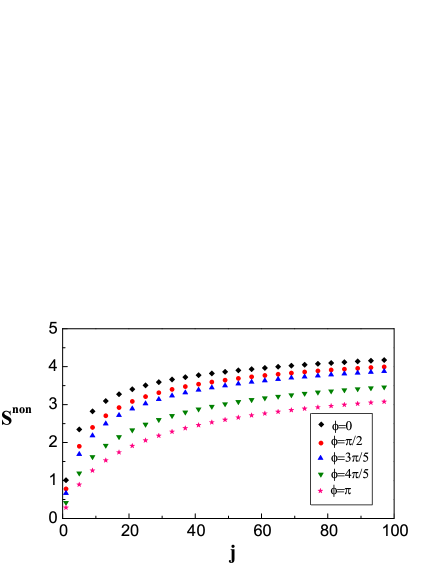
Figure 3: (Color online). The variations of the entropy of the cavity field, $S^{non}$, with passing times of the TLAPs, $j$, for different relative phases, $\phi=\{0,\pi/2,3\pi/5,4\pi/5,\pi\}$, and the other parameters of the state in Eq. (46) are $r_{1}=0.2$, $r_{2}=1$, $\alpha=\pi/3$, $\theta_{1}=3\pi/4$, $\theta_{2}=\pi/2$, $\varphi=0$.

Next, let us consider the influence of the relative phase in the coherent term $a_{23}$ of the TLAP on the work capability of the cavity field. As mentioned before, although the quantum correlations, QE and QD, have nothing to do with the relative phase in $a_{23}$ $(a_{32})$, it is very important to determine the constructive or the destructive interference in the work capability of cavity field as shown in Eq. (28) in the limit $\xi\rightarrow 0$. For case 2 with finite $\xi$ it is difficult to obtain explicit expressions of the average photon number and the entropy of the cavity, but we can demonstrate the effects of the relative phase on the entropy of the cavity field via numerical calculations. In terms of Eqs. (20) and (46) we plot the variations of the entropy of the cavity field, $S^{non}$, with passing times, $j$, for different relative phases, $\phi=\{0,\pi/2,3\pi/5,4\pi/5,\pi\}$ in Fig. 3 where the other parameters are: $r_{1}=0.2$, $r_{2}=1$, $\alpha=\pi/3$, $\theta_{1}=3\pi/4$, $\theta_{2}=\pi/2$, $\varphi=0$. From Fig. 3 we can see that for fixed passing time, $j$, the entropy of cavity field decreases with the relative phase $\phi$ for $\phi\in[0,\pi]$. In fact, when the relative phase ranges from 0 to $2\pi$ we can find that for fixed passing time, $j$, the entropy of cavity field $S^{non}$ is symmetric about $\phi=\pi$, i.e., $S^{non}(\pi-\phi)=S^{non}(\pi+\phi)$ with $\phi\in[0,\pi]$. Moreover, Fig. 3 also shows that for an arbitrary $\phi$ the entropy of the cavity field always increases with the passing times, $j$, and its increment for the neighboring twice passings decreases which means that the entropy, $S^{non}$, is convergent as expected.

Based on the above analysis, we can see that no matter whether there exist quantum correlations or not the reservoir’s coherence could have an effect on the work capability of the cavity. Moreover, it has been shown that although the relative phase is independent of the quantum correlations it has an important effect on the dynamics of cavity field. The constructive and destructive interferences could be induced to change the thermodynamic features of cavity field, such as the entropy and the average photon number of cavity, via controlling the relative phase. It is obvious that the reservoir’s coherence plays a central role in system’s work capability in our model, and it could be taken as an effective source of system’s work capability even in the absence of quantum correlations. This is our major result in this paper.

It is emphasized that the cavity is always in a nonequilibrium state with the TLAPs passing. As mentioned before, only for certain conditions $\hat{\rho}_{A}=\hat{\rho}_{B}$ and $a_{11}+a_{22}<a_{33}+a_{44}$ the steady state of the cavity in case 1 becomes a thermal equilibrium state. In general, the work capability refers to the entropy of the cavity field not to the average photon number. Roughly speaking, when the density matrix of the cavity keeps in diagonal distribution the average photon number of cavity has similar behavior as the entropy of cavity (i.e., when the average photon number of cavity increases the corresponding entropy of cavity will also increase), and it can also be used to describe the work capability of cavity. Strictly speaking, it is not precise to use the average photon number describing the potential work capability of cavity because it can not effectively determine the actual degree of work capability of cavity in a nonequilibrium state.

Especially, when the density matrix of the cavity has nondiagonal elements the change tendency of the average photon number of the cavity field can not always coincide with that of the entropy of the cavity field as shown in Fig. 2. Only for the cavity being in a thermal state although the average photon number denoted as $\bar{n}$ and the entropy denoted as $S$ are different physical quantities they may have similar behavior which can be explained as follows. As we know that the probabilities $P_{m}$ for the cavity field being in a thermal state with $m=0,1,2,...$ photons can be expressed as

$$P_{m}=\frac{\bar{n}^{m}}{(\bar{n}+1)^{m+1}},$$ (64)

which satisfy the normalization condition $\sum_{m}P_{m}=1$. Inserting Eq. (64) into the entropy expression of the cavity field $S=-\sum_{m}P_{m}\log_{2}P_{m}$ and after some calculations one obtains

$$S=(\bar{n}+1)\log_{2}(\bar{n}+1)-\bar{n}\log_{2}\bar{n}.$$ (65)

From Eq. (65) it is easy to verify that ${dS}/{d\bar{n}}>0$ which means that the entropy of the cavity field in a thermal state, $S$, is a monotonous increasing function of the average photon number, $\bar{n}$. So, both the average photon number and the entropy of the cavity field in the thermal state can be used to describe the work capability of cavity.

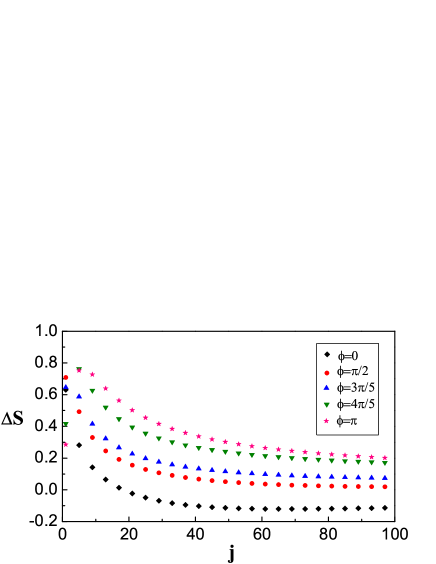
Figure 4: (Color online). The variations of the entropy difference of cavity field, $\triangle S$, with passing times of the TLAPs, $j$, for different relative phases, $\phi=\{0,\pi/2,3\pi/5,4\pi/5,\pi\}$, and the other parameters of the state in Eq. (46) are $r_{1}=0.2$, $r_{2}=1$, $\alpha=\pi/3$, $\theta_{1}=3\pi/4$, $\theta_{2}=\pi/2$, $\varphi=0$.

Thus, we argue that in general the proper physical quantity to measure the work capability of cavity is the entropy of cavity rather than the average photon number. In order to make this point more clearer we perform a thermalization on the cavity when the $j$th TLAP passes through the cavity, and keep the average photon number of the cavity unchanged, i.e., the energy of the cavity remains constant during the thermalization. Denote the average photon number and the density matrix of the cavity, after the $j$th passing, as ${\bar{n}_{j}}$ and ${\hat{\rho}_{j}}$ satisfying Eq. (20) and the state after thermalization as ${\hat{\rho}_{j}^{th}}$. Then, the thermal state of cavity, ${\hat{\rho}_{j}^{th}}$, can be expressed as

$${\hat{\rho}_{j}^{th}}=Z^{-1}\sum_{n^{\prime}=0}^{\infty}e^{-n^{\prime}/\bar{n}_{j}}|n{{}^{\prime}}\rangle\langle n{{}^{\prime}}|,$$ (66)

where $Z=1-e^{-1/\bar{n}_{j}}$ and $\bar{n}_{j}=\sum_{n=0}^{2j+1}n\rho_{nn}$ with $n$ and $\rho_{nn}$ respectively being the energy level and the corresponding probability distribution of the state $\hat{\rho}_{j}$. The entropy difference of the cavity, ${\triangle S}$, between the states before and after thermalization is given by

$${\triangle S}=S^{non}-S^{th},$$ (67)

where $S^{non}$ and $S^{th}$ independently correspond to the von Neumann entropy $S(\hat{\rho}_{j})$ and $S(\hat{\rho}_{j}^{th})$. Here, the entropy difference ${\triangle S}$ can effectively describe the deviation away from the corresponding thermal equilibrium. As an example, we choose the same parameters as that in Fig. 3, and plot the variations of the entropy difference of the cavity with the passing times $j$ for different relative phases $\phi=\{0,\pi/2,3\pi/5,4\pi/5,\pi\}$ in Fig. 4. From Fig. 4 we can see that during the evolution the entropy difference of the cavity may be larger or smaller than zero which depends on the passing times of the TLAPs, $j$, and the relative phase, $\phi$. That implies that the cavity might absorb heat from the reservoir $(\triangle S>0)$ or release heat to the reservoir $(\triangle S<0)$ during the thermalization process. Thus, it is the entropy of cavity actually describing the potential work capability of cavity not the average photon number except that the cavity reaches thermal equilibrium, and in this case, although the average photon number and the entropy are different physical quantities but they have similar behavior as shown in Eq. (65). This is consistent with the spirit demonstrated in another model Esposito most recently reported where the authors proposed a entropic motor by exploiting entropy to fuel an engine and showed that the generation of the entropic forces is surprisingly robust to local changes in kinetic and topological parameters.

IV summary and conclusions

In conclusion, we have studied the dynamics of cavity with a nonequilibrium reservoir consisting of a beam of identical TLAPs initially preparing in the general X-state, and have derived a quantum master equation. We have found that the coherence of a nonequilibrium reservoir consisting of TLAPs in the X-state plays a central role in the dynamics of cavity field. It has been shown that not only the constructive interference but also the destructive interference could be induced only by adjusting the relative phase with which the quantum correlations have nothing to do. Using this property a thermodynamic cycle with a single reservoir can be implemented only via controlling one external parameter, the relative phase. Meanwhile, we have also found that no matter whether the quantum correlations exist or not the coherence of reservoir could have contributions to the work capability of cavity. We, in the present paper, have clearly demonstrated that quantum coherence rather than quantum correlations can reflect the effects of reservoir on the system’s work capability effectively. In addition, we have also shown that the proper physical quantity to measure the potential work capability of cavity field is the entropy of cavity field rather than the average photon number except that the cavity arrives at thermal equilibrium, and in this case both of them can be used to describe the work capability of cavity field. This work might prompt further studies on how to use coherence as a thermodynamic resource, such as the study of coherence in the heat dissipation of atomic-scale junctions in most recent experiments Lee . Finally, it is also interesting to extend our present work to the Dicke model and some new results might be revealed which will be considered in the future work.

Appendix A The expressions of $f_{i}$

The parameters $f_{i}$, ($i=1,2,3,...,11$), in Eq. (20) are given by

$$f_{1}= a_{11}U_{11}(m)U_{11}(n)+a_{44}U_{44}(m)U_{44}(n)$$ (68)

$$+ (a_{22}+a_{33})[U_{22}(m)U_{22}(n)+U_{23}(m)U_{23}(n)]$$

$$+ (a_{23}+a_{32})[U_{22}(m)U_{23}(n)+U_{23}(m)U_{22}(n)],$$

$$f_{2}= (a_{22}+a_{33}+a_{23}+a_{32})U_{12}(m+1)U_{12}^{*}(n+1)$$

$$+ 2a_{44}U_{24}(m+1)U_{24}^{*}(n+1),$$

$$f_{3}= (a_{22}+a_{33}+a_{23}+a_{32})U_{42}(m-1)U_{42}^{*}(n-1)$$

$$+ 2a_{11}U_{21}(m-1)U_{21}^{*}(n-1),$$

$$f_{4}= a_{11}U_{41}(m-2)U_{41}(n-2),$$

$$f_{5}= a_{44}U_{14}(m+2)U_{14}(n+2),$$

$$f_{6}= a_{14}U_{11}(m)U_{14}(n+2),$$

$$f_{7}= a_{41}U_{14}(m+2)U_{11}(n),$$

$$f_{8}= 2a_{41}U_{24}(m+1)U_{42}^{*}(n-1),$$

$$f_{9}= 2a_{14}U_{24}(m-1)U_{42}^{*}(n+1),$$

$$f_{10}= 2a_{41}U_{44}(m)U_{41}(n-2),$$

$$f_{11}= 2a_{14}U_{44}(m-2)U_{41}(n),$$

where $U_{ij}(x)$, $(i,j=1,2,3,4)$ ($x$ is the nonnegative integer ) are expressed as

$$U_{11}(x)= 1+\frac{(x+1)[\cos g\tau\sqrt{2(2x+3)}-1]}{2x+3}$$ (69)

$$U_{44}(x)= 1+\frac{x[\cos g\tau\sqrt{2(2x-1)}-1]}{2x-1}$$

$$U_{22}(x)= U_{33}(x)=\frac{1}{2}{[\cos g\tau\sqrt{2(2x+1)}+1]}$$

$$U_{23}(x)= U_{32}(x)=\frac{1}{2}{[\cos g\tau\sqrt{2(2x+1)}-1]}$$

$$U_{14}(x)= \frac{\sqrt{x(x-1)}[\cos g\tau\sqrt{2(2x-1)}-1]}{2x-1}$$

$$U_{41}(x)= \frac{\sqrt{(x+1)(x+2)}[\cos g\tau\sqrt{2(2x+3)}-1]}{2x+3}$$

$$U_{12}(x)= =U_{13}(x)=-i\sqrt{x}\frac{\sin g\tau\sqrt{2(2x+1)}}{\sqrt{2(2x+1)}}$$

$$U_{21}(x)= =U_{31}(x)=-i\sqrt{x+1}\frac{\sin g\tau\sqrt{2(2x+3)}}{\sqrt{2(2x+3)}}$$

$$U_{24}(x)= =U_{34}(x)=-i\sqrt{x}\frac{\sin g\tau\sqrt{2(2x-1)}}{\sqrt{2(2x-1)}}$$

$$U_{42}(x)= =U_{43}(x)=-i\sqrt{x+1}\frac{\sin g\tau\sqrt{2(2x+1)}}{\sqrt{2(2x+1)}}.$$

References

- (1) Z. Ficek and S. Swain, Quantum Interference and Coherence: Theory and Experiments, Springer Series in Optical Sciences Vol. 100 (Springer Science, New York, 2005).
- (2) M.O. Scully, M.S. Zubairy, G.S. Agarwal, and H. Walther, Science 299, 862 (2003).
- (3) H.T. Quan, P. Zhang, and C.P. Sun, Phys. Rev. E 73, 036122 (2006).
- (4) J.Q. Liao, H. Dong, and C. P. Sun, Phys. Rev. A 81, 052121 (2010).
- (5) S.W. Kim and M.S. Choi, Phys. Rev. Lett. 95, 226802 (2005).
- (6) S. Pielawa, G. Morigi, D. Vitali, and L. Davidovich, Phys. Rev. Lett. 98, 240401 (2007).
- (7) A. Sarlette, J.M. Raimond, M. Brune, and P. Rouchon, Phys. Rev. Lett. 107, 010402 (2011).
- (8) J.F. Poyatos, J.I. Cirac, and P. Zoller, Phys. Rev. Lett. 77, 4728 (1996).
- (9) C.J. Myatt, B.E. King, Q.A. Turchette, C.A. Sackett, D. Kielpinski, W.M. Itano, C. Monroe, and D.J. Wineland, Nature (London) 403, 269 (2000).
- (10) S. Diehl, A. Micheli, A. Kantian, B. Kraus, H. P. Buchler, and P. Zoller, Nature Phys. 4, 878 (2008).
- (11) F. Verstraete, M.M. Wolf, and J.I. Cirac, Nature Phys. 5, 633 (2009).
- (12) Y.D. Wang and A.A. Clerk, arXiv:1301.5553.
- (13) G.S. Engel, T.R. Calhoun, E.L. Read, T.K. Ahn, T. Manal, Y.C. Cheng, R.E. Blankenship, and G.R. Fleming, Nature (London) 446, 782 (2007).
- (14) G. Panitchayangkoon, D. Hayes, K.A. Fransted, J.R. Caram, E. Harel, J. Wen, R.E. Blankenship, and G.S. Engel, Proc. Natl. Acad. Sci. U.S.A 107, 766 (2010).
- (15) S.F. Huelga and M.B. Plenio, Contemp. Phys. 54, 181 (2013).
- (16) J.L. Wu, F. Liu, J. Ma, R.J. Silbey, and J.S. Cao, J.Chem. Phys. 137, 174111 (2012).
- (17) J.L. Wu, R.J. Silbey, and J.S. Cao, Phys. Rev. Lett. 110, 200402 (2013).
- (18) I. Kassal, J.Y. Zhou, and S.R. Keshari, J. Phys. Chem. Lett. 4, 362 (2013).
- (19) A. Ishizaki and G.R. Fleming, Annu. Rev. Phys. Chem. 3, 333 (2012).
- (20) H. Lee, Y. C. Cheng, and G. R. Fleming, Science 316, 1462 (2007).
- (21) Y. C. Cheng and R. J. Silbey, Phys. Rev. Lett. 96, 028103 (2006).
- (22) E. Collini, C. Y. Wong, K. E. Wilk, P. M. G. Curmi, P. Brumer, and G. D. Scholes,Nature 463, 644 (2010).
- (23) S. Hormoz, Phys. Rev. E 87, 022129 (2013).
- (24) L. A. Correa, J. P. Palao, G. Adesso, and D. Alonso, Phys. Rev. E 87, 042131 (2013).
- (25) H.T. Quan, Y.X. Liu, C.P. Sun, and F. Nori, Phys. Rev. E 76, 031105 (2007)
- (26) H. Wang, S.Q. Liu, and J.Z. He, Phys. Rev. E 79, 041113 (2009).
- (27) N. Brunner, M. Huber, N. Linden, S. Popescu, R. Silva, and P. Skrzypczyk, arXiv:1305.6009v1.
- (28) A.L Grimsmo, Phys. Rev. A 87, 060302 (2013).
- (29) K. Funo, Y. Watanabe, and M. Ueda, Phys. Rev. A 88, 052319 (2013).
- (30) J.J. Park, K.H. Kim, T. Sagawa, and S.W. Kim, Phys. Rev. Lett. 111, 230402 (2013).
- (31) X. L. Huang, T. Wang, and X. X. Yi, Phys. Rev. E 86, 051105 (2012).
- (32) L. A. Correa, J. P. Palao, D. Alonso, G. Adesso, Scientific Reports. 4, 3949 (2014).
- (33) O. Abah and E. Lutz, arXiv:1303.6558v2.
- (34) P. Mehta and A. Polkovnikov, Ann. Phys. 332, 110 (2012).
- (35) R. Dillenschneider and E. Lutz, Europhys. Lett. 88, 50003 (2009).
- (36) T. Baumgratz, M. Cramer, and M.B. Plenio, arXiv:1311.0275v1.
- (37) M.O. Scully, Phys. Rev. Lett. 104, 207701 (2010).
- (38) M.O. Scully, K.R. Chapin, K.E. Dorfman, M.B. Kim, and A.y. Svidzinsky, Proc Natl Acad Sci USA 108, 15097 (2011).
- (39) P. Nalbach and M. Thorwart, Proc Natl Acad Sci USA 110, 2693 (2013).
- (40) K.E. Dorfman, D.V. Voronine, S. Mukame, and M.O. Scully, Proc Natl Acad Sci USA 110, 2746 (2013).
- (41) P. Filipowicz, J. Javanainen, and P. Meystre, Phys. Rev. A 34, 3077 (1986).
- (42) M.O. Scully and M.S. Zubairy, Quantum Optics (Cambridge University Press, Cambridge, 1997).
- (43) M.O. Scully and W.E. Lamb, Phys. Rev. 159, 208 (1967).
- (44) M. Orszag, Quantum Optics: Including Noise Reduction, Trapped Ions, Quantum Trajectories, and Decoherence (Springer, Berlin, 2007).
- (45) D. Meschede, H. Walther, and G. Müller, Phys. Rev. Lett. 54, 551 (1985).
- (46) F. Casagrande, M. Garavaglia, and A. Lulli, Opt. Comm. 151, 395 (1998).
- (47) J.D. Cresser, Phys. Rev. A 46, 5913 (1992).
- (48) J.D. Cresser and S.M. Pickles, Quan. and Semiclassical Optics 8, 73 (1996).
- (49) J. Bergou, L. Davidovich, M. Orszag, C. Benkert, M. Hillery, and M.O. Scully, Phys. Rev. A 40, 5073 (1989); J. Bergou and P. Kálmán, Phys. Rev. A 43, 3690 (1991).
- (50) E.S. Guerra, A.Z. Khoury, L. Davidovich, and N. Zagury, Phys. Rev. A 44, 7785 (1991).
- (51) M. Brune, J.M. Raimond, P. Goy, L. Davidovich, and S. Haroche, Phys. Rev. Lett. 59, 1899 (1987).
- (52) G. Rempe, F. Schmidt-Kaler, and H. Walther, Phys. Rev. Lett. 64, 2783 (1990).
- (53) W.K. Wootters, Phys. Rev. Lett. 80, 2245 (1998).
- (54) H. Ollivier and W.H. Zurek, Phys. Rev. Lett. 88, 017901 (2001).
- (55) C.Z. Wang, C.X. Li, L.Y. Nie, and J.F. Li, J. Phys. B: At. Mol. Opt. Phys. 44, 015503 (2011).
- (56) N. Golubeva, A. Imparato, and M. Esposito, Phys. Rev. E 88, 042115 (2013).
- (57) W. Lee, K. Kim, W. Jeong, L.A. Zotti, F. Pauly, J.C. Cuevas, and P. Reddy, Nature 498, 209 (2013).