Transfer arbitrary photon state along a cavity array without initialization

Abstract

We propose a quantum state transfer (QST) scheme that transfers any single-mode photon state along a one-dimensional coupled-cavity array (CCA). By building a map from QST in a CCA to that in a spin-$\frac{1}{2}$ chain, we show that all the previous results of QST schemes for the spin chain system find paralleled applications in that in the CCA system. Further more, high fidelity QST along a long CCA can be achieved for arbitrary initial states. Using numerical simulations we provide a visual presentation of the result: at some time $\tau$ the CCA system get high fidelity QST under different initial conditions. Finally we discuss possible experimental realizations of our QST scheme.

Introduction.

— Quantum state is the carrier of the information in quantum information and quantum computation. Transmitting quantum state from one location to another is one of the basic tasks in quantum information processing system. The most famous scheme of QST is quantum state teleportation Bennett et al. (1993), where the unknown state is teleported with the aid of one shared EPR pair between the sender and the receiver and 2 bits of classical information. This scheme indicates that quantum entanglement is a resource in QST. A more direct one is to transfer the unknown state through a shared quantum network Cirac et al. (1997); Bose (2003).

The simplest quantum network used to transfer quantum state is a one dimensional spin-$1/2$ spin chain, which is pioneered by Bose. Bose showed that the high fidelity of state transfer could be achieved through a long unmodulated spin chain. QST along an unmodulated spin chain can be perfect only when the length of the spin chain is less than $4$. For the chain of any length perfect QST can be achieved by modulating the coupling strengths between adjacent spins Christandl et al. (2004); Shi et al. (2005); Nikolopoulos et al. (2004a, b). Other schemes are also discussed such as only tuning the two end coupling strengths to get high fidelity QST Wójcik et al. (2005); Campos Venuti et al. (2007); Li et al. (2005); Giampaolo and Illuminati (2010); Gualdi et al. (2008); Yao et al. (2011); Bruderer et al. (2012), QST without initialization Di Franco et al. (2008); Markiewicz and Wieśniak (2009), and generalizing to the high spin QST Bayat and Karimipour (2007); Qin et al. (2013). Number-Theoretic relation between QST and the length of one-dimension spin chain is found in Ref. Godsil et al. (2012).

In addition, schemes based on cavity quantum electrodynamics are also reported. An initial proposal is to transfer the state of a qubit from a cavity-atom system to another one through an optical fiber connecting the two cavities Cirac et al. (1997); Ritter et al. (2012).

In this paper we propose a QST scheme that transfers any single-mode photon state along a one-dimensional CCA. All the previous results got in the spin chain system mentioned above are applicable in our scheme and the initialization step is not needed. It is naturally a high dimension QST scheme. With the development of technology of producing high quality cavities Armani et al. (2003); Yariv et al. (1999); Akahane et al. (2003) and the control of the photons in the cavity Kuhr et al. (2007); Wang et al. (2008); Brune et al. (2008); Johnson et al. (2010); Sayrin et al. (2011), the realization of our scheme is possible.

This article is organized as follows. First we propose the QST scheme, where the Hamiltonian of the system is given. Next we analyse the fidelity of QST in our scheme and give the condition of perfect QST. Then we solve the dynamic problem about fidelity. After that we simulate the QST using our scheme in three cases: uniform coupling CCA, perfect modulated CCA and the CCA with coupling strengths in the ballistic regime. Finally we give some discussion on experimental realization of our scheme.

Scheme and Analysis.

— The system of our scheme is a CCA as depicted in Fig. 1. Every cavity has the same cavity mode $\omega$. Photons can hop between adjacent cavities due to the overlap of the light mode Hartmann et al. (2006). The Hamiltonian is given by

$$H=\hbar\omega\sum_{n=1}^{N}\hat{a}_{n}^{\dagger}\hat{a}_{n}+\sum_{n=1}^{N-1}J_{n}(\hat{a}_{n}^{\dagger}\hat{a}_{n+1}+\hat{a}_{n}\hat{a}_{n+1}^{\dagger}),$$

where $\omega$ is the frequency of the cavity mode, $J_{n}$s are the coupling strengths between adjacent cavities, which can be adjusted by changing the thickness of the mirrors.

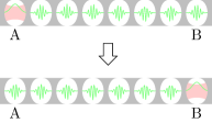
Figure 1: Our quantum communication protocol. Initially prepare the quantum state needed to communicate in the first cavity (cavity A). After a while, the state transfer to the other end of the array (cavity B). The Gauss curve means the transmitted photon state. The wavy lines in the cavities represent the arbitrary state of single-mode photon.

The process of the QST along the CCA is as follows. First, the state we want to transfer is encoded on the photons in the first cavity (cavity $A$) as $|\phi_{1}\rangle=f(\hat{a}^{\dagger}_{1})|0\rangle$ which is unknown in many cases. Next we allow the unitary evolution controlled by the Hamiltonian $H$ for a time period $t$. Then we check whether the unknown state has been transferred to another end of the array (cavity $B$ ($N$)).

Firstly we consider the fidelity which is defined as $\langle\phi_{N}|\rho_{N}(t)|\phi_{N}\rangle$ to characterize the quality of the QST. Let the initial state of the system as

$$|\psi_{0}\rangle\langle\psi_{0}| =f(\hat{a}_{1}^{\dagger})|0\rangle\langle 0|f^{*}(\hat{a}_{1})\otimes\rho_{2-N}.$$

Then the fidelity of the system at time $t$ is

$$\mathcal{F}(t)= \tr\left(\langle 0|f^{*}(\hat{a}_{N}(t))f(\hat{a}_{1}^{\dagger})|0\rangle\langle 0|f^{*}(\hat{a}_{1})\right.$$

$$\ \ \ \ \left.\otimes\rho_{2-N}f(\hat{a}_{N}^{\dagger}(t))|0\rangle\right),$$

where $\hat{a}_{N}(t)$ is operator $\hat{a}_{N}$ in the Heisenberg picture, that is $\hat{a}_{N}(t)=\hat{U}^{\dagger}(t)\hat{a}_{N}\hat{U}(t)$ with $\hat{U}(t)$ as time evolution operator. If at time $\tau$ we have the relation $\hat{a}_{N}\left(\tau\right)=\hat{a}_{1}$, then we get the conclusion that at time $\tau$ we have a perfect transfer, $\mathcal{F}(\tau)=1$. In other words, to get a perfect photon state transfer means to get a time $\tau$ that $\hat{a}_{N}(\tau)=\hat{a}_{1}$. It can be easily verified by noting that the expect value of the any operator in the $N$-th cavity at time $\tau$ is equal to that of the operator in the first cavity at initial state, e.g., $\langle\hat{a}_{N}^{\dagger}\hat{a}_{N}(\tau)\rangle=\langle\hat{a}_{1}^{\dagger}\hat{a}_{1}(0)\rangle$.

Now we analyse the dynamics of $\hat{a}_{N}^{\dagger}(t)$, which satisfies the Heisenberg equation

$$\frac{d\hat{a}_{N}^{\dagger}\left(t\right)}{dt}=i\left[H,\,\hat{a}_{N}^{\dagger}(t)\right].$$ (1)

First we note that the set, $\{\hat{a}_{n}^{\dagger}|{n}=1,\,2,\,3,\cdots,\,N\}$, is closed under the action $[H,\cdot]$. So $\hat{a}_{N}^{\dagger}(t)$ can be expanded as

$$\hat{a}_{N}^{\dagger}\left(t\right)=\sum_{n=1}^{N}\alpha_{n}(t)\hat{a}_{N+1-n}^{\dagger}.$$ (2)

Now we come to the solution of $\hat{a}_{N}^{\dagger}(t)$, which is determined from the Heisenberg equation for $\hat{a}_{N}^{\dagger}$:

$$\frac{dA}{dt}=i(G+\hbar\omega)A,$$ (3)

where $A=[\alpha_{1}(t),\,\alpha_{2}(t),\,\cdots,\alpha_{N}]^{T}$ with $T$ being the transpose operation, $G$ is a tri-diagonal matrix

$$G=\begin{bmatrix}0&J_{N-1}&0&0&\cdots\\ J_{N-1}&0&J_{N-2}&0&\cdots\\ 0&J_{N-2}&0&J_{N-3}&\cdots\\ 0&0&J_{N-3}&0&\cdots\\ \vdots&\vdots&\vdots&\vdots&\vdots\end{bmatrix}.$$

The initial condition is $A(0)=[1,\,0,\,\cdots,0]^{T}$. To solve the differential equations we can apply the Laplace transformation on the both sides of equation as it was done in Ref. Liu and Zhou (2013). Note that multiplying the both sides of Eq. (3) by $i$, we can rewrite it as $i\frac{dA}{dt}=\hat{H}_{new}A$, which has the same formation as Schrödinger equation with $\hat{H}_{new}=-(G+\hbar\omega)$. The new Hamiltonian $\hat{H}_{new}$ is in an $N$-dimensional Hilbert space, which is much more tractable than the original Hamiltonian $\hat{H}$ that is in the $D^{N}$-dimensional Hilbert space. $A$ is the wave function of the new Hamiltonian, and we denote it as $|A\rangle$. That is the operator $a^{\dagger}_{N}(t)$ is represent as a vector $|A\rangle$ in the Hilbert space of the new Hamiltonian. It is worth mentioning that the reason of the less Hilbert space is that the number of the set, which contains $A_{N}^{\dagger}$ and is closed under the operator $[H,\cdot]$, is only $N$, rather than the excitation number conservation. This can be seen clearly in the XY Hamiltonian with the coupling strength that can’t conserve the excitation number Liu and Zhou (2013).

In the uniform condition, $J_{n}=1$, the eigenvalues and eigenstates of the new Hamiltonian $\hat{H}_{new}$ are $E_{n}=-2\cos\frac{\pi n}{N+1}-\hbar\omega$, with $n=1,\cdots,N$, and $\langle l|\phi_{n}\rangle=\sqrt{\frac{2}{N+1}}\sin\frac{\pi nl}{N+1}.$ We consider the question that what is the sate of the new system at the given time $t$. The Hamiltonian of the system is $\hat{H}_{new}$ and the initial state is $|A_{0}\rangle=[1,0,\cdots,0]^{T}$. Using the Schrödinger equation we know

$$|A(t)\rangle=\sum_{n}\exp(-iE_{n}t)|\phi_{n}\rangle\sqrt{\frac{2}{N+1}}\sin\frac{\pi n}{N+1}.$$

The last element of the state is

$$\alpha_{N}(t)=\sum_{n}(-1)^{n-1}\frac{2}{N+1}\exp(-iE_{n}t)\sin^{2}\frac{\pi n}{N+1}.$$

From Ref. Godsil et al. (2012) we know that if and only if the number of length is $N=p-1,$ $2p-1$, where $p$ is a prime, or $N=2^{m}-1$ (for convenience we call it pretty good length condition), there is a time $\tau$ that $\exp(-i\mathcal{E}_{n}t)\thickapprox(-1)^{n-1}\gamma,$ where $\gamma=1$ if $N\equiv 1\mod 4$, $\gamma=-1$ if $N\equiv 3\mod 4$, $\gamma=\pm i$ if $N$ is even, and $\mathcal{E}_{n}=E_{n}+\hbar\omega$.

So we have $\alpha_{N}(\tau)\thickapprox\gamma e^{i\hbar\omega\tau}$. From $|\gamma e^{i\hbar\omega\tau}|=1,$ and the normalization of the state we get that $\alpha_{1}(\tau)\thickapprox\alpha_{2}\left(\tau\right)\thickapprox\cdots\thickapprox\alpha_{N-1}(\tau)\thickapprox 0$. So at the time $\tau$ we have

$$\hat{a}_{N}^{\dagger}\left(\tau\right)\thickapprox\gamma e^{i\hbar\omega\tau}\hat{a}_{1}^{\dagger}.$$

As for the phase $\gamma e^{i\hbar\omega\tau}$, we can adjust the cavity mode to a proper value $\omega_{\tau}$ that make $\gamma{e}^{i\hbar\omega_{\tau}\tau}=1$. So the get the conclusion that we get pretty good state transfer (PGST) at time $\tau$ if the length of the cavities satisfies the pretty good length condition and the cavity mode is $\omega_{\tau}$. Compared with the PGST in spin chains we don’t need the initialization of the cavities or the single excitation condition. In XY spin chains system QST is proportional to the parity of the initial state Liu and Zhou (2013), while in the CCA system if we can achieve perfect QST at time $\tau$ then the initial state of cavities $2-N$ have nothing to do with QST at the perfect time. The reason is that in XY spin chain system the operators in first site is bound with the other part of system by $X_{1}(Y_{1})Z_{2-N}$ while in the CCA system $\hat{a}_{1}^{\dagger}$ is standalone in the Heisenberg equation related with the operators of the $N$-th site.

For the general case that $J_{n}$s are not uniform, $\alpha_{N}$ is provided in ref. Liu and Zhou (2013) as

$$\frac{\alpha_{N}(t)}{\det A_{N}^{(N)}}=\begin{cases}\sum_{i=1}^{M}\frac{\sin(q_{i}t)}{q_{i}\prod_{j\neq i}(q_{j}^{2}-q_{i}^{2})}&\text{for }N=2m,\\ \sum_{i=0}^{M}\frac{\cos(s_{i}t)}{\prod_{j\neq i}(s_{j}^{2}-s_{i}^{2})}&\text{for }N=2m+1,\end{cases}$$ (4)

where $A=p-G$ with $p$ as Laplace complex argument, $A_{N}^{(N)}$ is the matrix $A$ whose $N$-th column vector is replaced by $A(0)$. $q$ and $s$ are roots of $\det A_{N}^{(N)}$. $m$ is an integer. When $\alpha_{N}(\tau)=1$ perfect QST is got.

Numerical simulation.

— Now we numerically simulate the QST in the unmodulated CCA and show its result in Fig. 2. The system we simulate has length $N=5$ with coupling strength $J_{n}=1$. Here we choose units such that $\hbar=1$. It shows that at time $\tau=21.8$, which requires $\omega(k)=\frac{2k\pi}{\tau}$, $k=0,1,2,\cdots$, we get a good fidelity $F(\tau)=0.9999$, for any initial state of the chain $2-N$ and the sent state. The first line (red one) simulates the fidelity of QST with the initial state of the cavities $2-N$ being $|0000\rangle$ and the sent state being the coherent state $|\alpha\rangle=e^{-|\alpha|^{2}/2}e^{\alpha a^{\dagger}}|0\rangle$, $\alpha=1$. The initial state of cavities $2-N$ for the other two lines (green and blue ones) are $|1000\rangle$, $|1100\rangle$ and the sent states are $\frac{1}{\sqrt{3}}(|0\rangle+|1\rangle+|2\rangle)$ and $\frac{1}{\sqrt{14}}(|0\rangle+|1\rangle+|2\rangle)$, respectively. The $\omega$ we choose is $\omega(1)=0.288$.

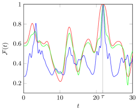
Figure 2: (Color online) Numerical simulation of the fidelity $F(t)$ of QST for $N=5$ as a function of $t$ in uniform coupling case ($J_{i}=1$). The initial states of the three lines are $|\alpha\rangle|0000\rangle$, $\frac{1}{\sqrt{3}}(|0\rangle+|1\rangle+|2\rangle)|1000\rangle$, $\frac{1}{\sqrt{14}}(|0\rangle+2|1\rangle+3|2\rangle)|1100\rangle$ respectively. $|\alpha\rangle=e^{-|\alpha|^{2}/2}e^{\alpha a^{\dagger}}|0\rangle$ is coherent state, here $\alpha=1$.

Note that other conclusions of QST in the spin chain system are also applicable in the CCA system. As we know that the spin chains with modulated coupling strength have the prefect QST when the parity of the initial state (except the first spin) is 1. The modulated coupling strengths are $J_{n}=J_{n}^{[k]}=\sqrt{n(N-n)}$ for even $n$ and $J_{n}=J_{n}^{[k]}=\sqrt{(n+2k)(N-n+2k)}$ for odd $n$, where $k\in\{0,\,1,\,2,\cdots\}$ Christandl et al. (2004); Shi et al. (2005). For the case $k=0$, the matrix $G$ is identical to the representation of the Hamiltonian $H$ of a fictitious spin $S=\frac{1}{2}(N-1)$ particle: $H=2S_{x}$, where $S_{x}$ is angular momentum in $x$ direction Christandl et al. (2004).

Now we consider the case that the coupling strengths are the prefect modulated ones with $k=0$. So the new Hamiltonian is $H_{new}=-(2S_{x}+\hbar\omega)$. $\alpha_{N}(t)$ can be written directly as

$$\alpha_{N}\left(t\right)=\left[i\sin\left(t\right)\right]^{N-1}e^{i\hbar\omega t}.$$

So at time $\tau=\frac{\pi}{2}$, $|\alpha_{N}(t)|=1$. The required frequency is $\omega=4k+1-N$, $k=0,1,2,\cdots$. In Fig. 3 we demonstrate the fidelity $\mathcal{F}(t)$ versus $t$ for the modulated CCA system with length $N=8$. The sent state is $\frac{1}{\sqrt{3}}(|0\rangle+|1\rangle+|2\rangle)$, and the initial states of cavity $2-N$ are thermal state $\frac{e^{-\beta{H}}}{Z}$ with $\beta=0.5,1,10,20$ and the $\omega=17,9,5,1$ respectively. It shows that at time $\tau=\pi/2$ QST of the CCA system with modulated coupling strength is perfect whatever the initial state of cavities $2-N$ are. Fig. 3 also depicts that different frequencies, $\omega$s, result in the different oscillation times in one period in the fidelity aspect as expected.

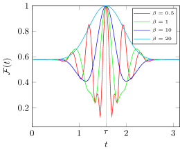
Figure 3: (Color online) Numerical simulation of the fidelity $F(t)$ of QST for $N=8$ as a function of $t$ in the modulated coupling case ($J_{n}=\sqrt{(n+2k)(N-n+2k)}$) for different initial states. The initial states are $\rho_{1}\otimes\rho_{2-8}s$, and $\rho_{1}=\frac{1}{3}(|0\rangle+|1\rangle+|2\rangle)(\langle{0}|+\langle{1}|+\langle{2}|)$.

In the uniform XX spin channel, perfect QST can be achieved by tuning down the two end coupling strengths limited to zero for arbitrary length $N$ Yao et al. (2011). But the optimal time of perfect QST becomes long as end coupling strengths decreasing. There is a regime, which is called ballistic regime, that $0<J_{end}<1$ ( the uniform coupling strength is set to 1) the fidelity of QST is high and the transmission time is $t\sim N$ Banchi et al. (2011).

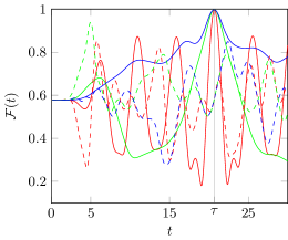
Figure 4: (Color online) Numerical simulation of the fidelity $F(t)$ of QST for $N=8$ as a function of $t$ in the ballistic regime case ($J_{1}=J_{7}=0.3$, $J_{n\neq 1,7}=1$) for different initial states and photon frequency $\omega$ (solid line). The initial states are $\rho_{1}\otimes\rho_{2-8}s$, $\rho_{1}=\frac{1}{3}(|0\rangle+|1\rangle+|2\rangle)(\langle{0}|+\langle{1}|+\langle{2}|)$, $\rho_{2-8}$s are thermal state with $\beta=20$ (red line), $|1000000\rangle$ (green line), $|1100000\rangle$ (blue line), respectively. And the corresponding photon frequencies are $1.29$, $0.379$, $0.076$. The dashed lines depict the corresponding fidelity in the uniform coupling system.

In Fig. 4 we simulate the QST of CCA system with length $N=8$ at the ballistic regime, $J_{1}=J_{7}=0.3$, depicted by solid lines. The dashed lines are the corresponding QST of the system with uniform coupling strength, $J_{n}=1$ with the same initial states. It shows that at time $\tau=20.7$ the system at ballistic regime get fidelity larger than $0.99$, while the uniform coupling system get some mediocre fidelity.

Experimental Realization.

— Our proposal can be realized using the experimental realization mentioned in ref. Hartmann et al. (2006) without atoms in the cavities. Toroidal micro-cavities can be produced with high precision and in large number on a chip. These cavities have a very high Q-factor ($>10^{8}$) for light that is trapped as whispering gallery modes and are coupled via tapered optical fibers Armani et al. (2003). Another promising candidate for an experimental realization is photonic crystals Yariv et al. (1999); Akahane et al. (2003). The technology preparing the coherent or Fock photon state in the cavity and counting the photon number Kuhr et al. (2007); Wang et al. (2008); Brune et al. (2008); Johnson et al. (2010); Sayrin et al. (2011) can be used to compute the fidelity of the QST of photon state.

Conclusion.

— In summary, we propose a QST scheme using a CCA system to transfer any single-mode photon state from one end of the array to the opposite end. Our analysis shows that all the results of QST schemes for spin chain system are applicable in our scheme and that pretty good QST of any single-mode photon state along the CCA system can be achieved for arbitrary initial states. Generally there will be a phase difference between the basis with different photon number. We eliminate this phase difference by choose the proper cavity mode frequency $\omega$ depending on transfer time $\tau$. We numerically simulate the schemes in three cases: uniform coupling CCA, perfect modulated CCA and the CCA with coupling strengths in ballistic regime. In every case we use different initial states and sent states, and the expected results are got. Using the technology of producing high quality cavity array and precisely preparing and measuring photon state in a cavity, our scheme of QST along a CCA may be realized in the near future.