Preserving information from the beginning to the end of time in a Robertson-Walker spacetime

Abstract

Preserving information stored in a physical system subjected to noise can be modeled in a communication-theoretic paradigm, in which storage and retrieval correspond to an input encoding and output decoding, respectively. The encoding and decoding are then constructed in such a way as to protect against the action of a given noisy quantum channel. This paper considers the situation in which the noise is not due to technological imperfections, but rather to the physical laws governing the evolution of the universe. In particular, we consider the dynamics of quantum systems under a 1+1 Robertson-Walker spacetime and find that the noise imparted to them is equivalent to the well known amplitude damping channel. Since one might be interested in preserving both classical and quantum information in such a scenario, we study trade-off coding strategies and determine a region of achievable rates for the preservation of both kinds of information. For applications beyond the physical setting studied here, we also determine a trade-off between achievable rates of classical and quantum information preservation when entanglement assistance is available.

Keywords: Quantum fields in curved spacetime, quantum communication, trade-off coding

1 Introduction

Data storage is relevant not only for accomplishing tasks in our day-to-day lives but also to keep track of our history. Information can be stored on various physical media, ranging from modern compact disks to ancient papyrus. A fundamental goal of information storage is to preserve it for the longest possible time in a reliable way. That obviously depends on the used technology. However, even if we have achieved a perfect or ideal implementation of a given technology, we should realize that there are limitations on preserving information. These limitations are posed by physical theories and ultimately result from the evolution of the universe itself, which can cause unavoidable effects to any physical system.

To address the issue of determining these fundamental limits, we require the theory of general relativity as well as that of quantum information. Very recently the interconnections between these two fields have received increased interest. Several previous works have developed a theory of communication between a sender and a receiver in relativistic settings [2, 5, 22, 19, 6, 4] or in situations involving black holes [3, 15].

In this paper, we investigate how well information stored in the remote past is preserved when going to the far future, by assuming evolution of the universe in a Robertson-Walker (RW) spacetime. Our main results are 1) that the noise imparted to spin-$\frac{1}{2}$ particles by the evolution of the universe is equivalent to an amplitude damping channel, and so we then 2) determine achievable rates for the simultaneous communication of classical and quantum information over this channel. As a result, we can interpret these rates to be achievable rates for the storage of classical and quantum information from the early past to the far future in a Robertson-Walker spacetime.

The RW spacetimes are a reasonable description of the dynamics of the late universe, which, at large scale, appear to be homogeneous and isotropic. Most cosmological models are special cases of RW spacetimes [1]. When considering a quantum matter field evolving through a dynamical spacetime, the concept of the vacuum cannot be considered unique any longer. Indeed, to detect the presence of quanta it is also necessary to specify the details of the quantum measurement process, and in particular, the state of motion of the measuring device. Particles possess an essential observer-dependent quality, so that they can be observed on some detectors and not others. Also, we can define positive and negative energy solutions of differential equations governing matter fields only if the spacetime structure is invariant under the action of a time-like Killing vector field [24]. This is certainly true for Minkowski spacetime, and a RW universe which is Minkowskian in the early past and in the far future is a suitable choice. The simplest, nevertheless insightful, choice we can make is a 1+1 RW spacetime.

There, we can consider any quantum state of the matter field before the expansion of the universe begins and define, without ambiguity, its particle content. We then let the universe expand and check how the state looks once the expansion is over. The overall picture can be thought of as a noisy channel into which some quantum state is fed. Once we have defined the quantum channel emerging from the physical model, we will be looking at the usual communication task as information transmission over the channel. Since we are interested in the preservation of any kind of information, we shall consider the trade-off between the different resources of classical and quantum information.

The rest of the paper is organized as follows. In the next section, we discuss the physical model and show how the noise imparted to spin-$\frac{1}{2}$ particles is equivalent to an amplitude damping channel, which has been well studied in quantum information theory [25]. In the section thereafter, we calculate achievable rates for the simultaneous communication of classical and quantum information over this channel. We then conclude with a summary of our results and a discussion of some open questions. Appendixes A and B are devoted to prove the main results. There we also determine a trade-off between achievable rates of classical and quantum information preservation when entanglement assistance is available, which might be useful for applications beyond the physical setting studied in this paper.

2 The physical model

2.1 Robertson-Walker spacetime

The geometry of a RW spacetime, considered here for the sake of simplicity of 1+1 dimensions, is described by the line element

$$ds^{2}=[a(\tau)]^{2}(-d\tau^{2}+dx^{2}),$$

which represents the varying distance between two spacetime points, depending on the conformal scale factor $a(\tau)$. The so-called conformal time $\tau$ is a function depending on the cosmological time $t$, defined by $\tau=\int a^{-1}(t)dt$. The spatial coordinate is denoted by $x$. Now consider an expanding universe with Minkowskian spacetime in the early past and in the far future filled with a Dirac field (that is, with matter made of spin-$\frac{1}{2}$ particles). We can associate a Hilbert space to each of the two regions with suitable basis vectors. The dynamics of the matter fields $\psi$ of mass $m$ are governed by the Dirac equation expressed in covariant form

$$(\tilde{\gamma}^{\mu}D_{\mu}+m)\psi=0.$$ (1)

The index $\mu$ runs from $0$ to $1$ and the Einstein sum rule over repeated indices is used. Furthermore, $\tilde{\gamma}^{\mu}\equiv[a(\tau)]^{-1}\gamma^{\mu}$ with $\gamma^{\mu}$ the $2\times 2$ matrices representing Dirac algebra. Finally, $D_{\mu}$ is the covariant derivative [1].

We look for solutions of (1), writing $\psi=a^{-1/2}(\gamma^{\nu}\partial_{\nu}-M)\varphi$, with $M=ma(\tau)$, so to have

$$g^{\mu\nu}\partial_{\mu}\partial_{\nu}\varphi-\gamma^{0}\dot{M}\varphi-M^{2}\varphi=0,$$ (2)

with $g^{\mu\nu}$ being the flat metric as opposed to the actual spacetime metric $\tilde{g}^{\mu\nu}=[a(\tau)]^{-2}g^{\mu\nu}$. Moreover, given flat spinors $u$ and $v$ satisfying $\gamma^{0}u=-iu$ and $\gamma^{0}v=iv$, we set

$$\varphi^{(-)}\equiv N^{(-)}f^{(-)}(\tau)ue^{ikx},$$ (3)

$$\varphi^{(+)}\equiv N^{(+)}f^{(+)}(\tau)ve^{ikx},$$ (4)

with $k$ the momentum. Inserting (3), (4) into (2), the functions $f^{(\pm)}$ must obey the differential equation

$$\ddot{f}^{(\pm)}+\left(k^{2}+M^{2}\pm i\dot{M}\right)f^{(\pm)}=0.$$ (5)

Define $f^{(\pm)}_{in/out}$ and ${f^{(\pm)}}^{*}_{in/out}$ the solutions behaving as positive and negative frequency modes with respect to conformal time $\tau$ near the asymptotic past/future, i.e. $\dot{f}^{(\pm)}_{in/out}(\tau)\approx-iE_{in/out}f^{(\pm)}_{in/out}(\tau)$ with

$$E_{in/out}\equiv\sqrt{k^{2}+M_{in/out}^{2}},\quad M_{in/out}\equiv ma(\tau\to+/-\infty).$$

Then we can introduce spinors that behave like positive and negative energy spinors, respectively, in the asymptotic regions:

$$U_{in/out}(k,x,\tau) \equiv N^{(-)}(\gamma^{\nu}\partial_{\nu}-M)f^{(-)}_{in/out}(\tau)ue^{ikx},$$ (6)

$$V_{in/out}(k,x,\tau) \equiv N^{(+)}(\gamma^{\nu}\partial_{\nu}-M){f^{(+)}}^{*}_{in/out}(\tau)ve^{-ikx},$$ (7)

with normalization constants

$$N^{(+)}=N^{(-)}=\left[\frac{E_{in/out}-M_{in/out}}{2k^{2}M_{in/out}}\right]^{1/2}.$$

Now the solutions of (1) can be expanded over (6) and (7) as

$$\psi(x,\tau) =\int dk\;a^{-1/2}(\tau)\left[a_{in}(k)U_{in}(k,x,\tau)+b_{in}^{{\dagger}}(k)V_{in}(k,x,\tau)\right],\quad\mathrm{or}$$

$$\psi(x,\tau) =\int dk\;a^{-1/2}(\tau)\left[a_{out}(k)U_{out}(k,x,\tau)+b_{out}^{{\dagger}}(k)V_{out}(k,x,\tau)\right].$$

The coefficients appearing in such expansions are $in$-$out$ ladder operators for particles and antiparticles ($a$, $a^{\dagger}$ and $b$, $b^{\dagger}$ respectively). They are connected by Bogoliubov transformations [10]

$$a_{out}(k) =\alpha(k)\,a_{in}(k)-\beta(k)\,b_{in}^{{\dagger}}(-k),$$ (8)

$$b_{out}^{{\dagger}}(-k) =\beta^{\ast}(k)\,a_{in}(k)+\alpha^{\ast}(k)\,b_{in}^{{\dagger}}(-k),$$ (9)

where $\alpha$, $\beta\in\mathbb{C}$, such that $|\alpha|^{2}+|\beta|^{2}=1$ and $\alpha\beta^{\ast}-\alpha^{\ast}\beta=0$. Notice that such transformations do not mix different momentum solutions, and so we can safely focus on a single momentum and omit the dependence on $k$. Therefore, any particle (antiparticle) quantum state lives in a 2-dimensional Hilbert space with orthonormal basis $\{|0\rangle,|1\rangle\}$ denoting absence or presence of a particle (antiparticle). The Bogoliubov coefficients are linked to physical quantities by $|\beta|^{2}=n/2$, where $n$ is the density of particles for the mode under consideration ($0\leq n\leq 2$).

The transformations (8), (9) come from a unitary operator that can be written as

$$U=\exp\left[r\left(e^{-i\vartheta}b^{{\dagger}}_{in}a_{in}^{{\dagger}}-e^{i\vartheta}a_{in}b_{in}\right)\right],$$ (10)

where the parameters $r$ and $\vartheta$ are related to $\alpha$ and $\beta$ of Eqs.(8) and (9) by $\alpha=\cos r$ and $\beta=-e^{-i\vartheta}\sin r$.

2.2 Robertson-Walker dynamics induces amplitude damping channel

Assuming to have access to particles in the out region only, the antiparticles will play the role of an environment which is initially in the vacuum. Hence, from (10), we can single out a completely positive trace preserving linear map from $in$ particle states to $out$ particle states, given by

$$\rho\mapsto\mathcal{A}(\rho)=\mathrm{tr}_{-p}\left[U\left(\rho\otimes|0\rangle_{-p}\langle 0|\right)U^{{\dagger}}\right]\,,$$ (11)

where $U$ is given by (10) and $\mathrm{tr}_{-p}$ stands for the partial trace over antiparticles. In terms of the so-called Kraus representation, we have that

$$\mathcal{A}(\rho)=\sum_{j=0,1}K_{j}\rho K_{j}^{{\dagger}},$$

where $K_{j}={}_{-p}\langle j|U|0\rangle_{-p}$ follows from (10)

$$K_{0} =I+(\cos r-1)a_{in}a_{in}^{{\dagger}},$$

$$K_{1} =e^{-i\vartheta}\sin r\,a_{in}^{{\dagger}}.$$

Expressing them in terms of outer products of particles states

$$K_{0} =\left|1\right\rangle\left\langle 1\right|+\sqrt{\eta}\left|0\right\rangle\left\langle 0\right|,$$ (12)

$$K_{1} =\sqrt{1-\eta}\left|1\right\rangle\left\langle 0\right|,$$ (13)

we may observe that the quantum channel map $\mathcal{A}$ is an amplitude damping channel with the so-called transmissivity $\eta\in[0,1]$ related to the physical observable $n$ by

$$\eta=\cos^{2}r=1-\frac{n}{2}.$$ (14)

We now consider the toy model introduced in [10], having the following conformal scale factor

$$a(\tau)=1+\epsilon(1+\tanh\rho\tau)\,.$$ (15)

The real and positive parameters $\epsilon$ and $\rho$ control the total volume and the rapidity of expansion of the universe, respectively. In the two asymptotic regions $in$ and $out$, we have that $a(\tau\rightarrow-\infty)=1$ and $a(\tau\rightarrow+\infty)=1+2\epsilon$, respectively.

Inserting (15) into (5) we get

$$\ddot{f}^{(\pm)}+\left[k^{2}+m^{2}(1+\epsilon(1+\tanh\rho\tau))^{2}\pm\frac{im\rho\epsilon}{\cosh^{2}\rho\tau}\right]f^{(\pm)}=0.$$

Solutions of this equation can be found as [10]

$$f_{in}^{(\pm)}(\tau)=e^{(-iE_{+}\tau-\frac{i}{\rho}E_{-}\ln(2\cosh\rho\tau))}$$

$$\hskip 36.98866pt\times\ _{2}{\sf F}_{1}\left(1+i\frac{E_{-}\pm m\epsilon}{\rho},i\frac{E_{-}\mp m\epsilon}{\rho},1-i\frac{E_{in}}{\rho},\frac{1+\tanh\rho\tau}{2}\right),$$

$$f_{out}^{(\pm)}(\tau)=e^{(-iE_{+}\tau-\frac{i}{\rho}E_{-}\ln(2\cosh\rho\tau))}$$

$$\hskip 36.98866pt\times\ _{2}{\sf F}_{1}\left(1+i\frac{E_{-}\pm m\epsilon}{\rho},i\frac{E_{-}\mp m\epsilon}{\rho},1+\frac{i}{\rho}E_{out},\frac{1-\tanh\rho\tau}{2}\right)\,,$$

with ${}_{2}{\sf F}_{1}$ denoting the ordinary hypergeometric function and

$$E_{\pm}\equiv\frac{E_{out}\pm E_{in}}{2}\,.$$

Since $f^{(\pm)}_{in/out}(\tau)$ and ${f^{(\pm)}}_{in/out}^{*}(\tau)$ are positive and negative frequency modes in asymptotic regions, we can write the Bogoliubov transformation between them as follows:

$$f_{in}^{(\pm)}(\tau)=A^{(\pm)}(k)f_{out}^{(\pm)}(\tau)+B^{(\pm)}(k){f_{out}^{(\mp)}}^{*}(\tau)\,.$$

Using linear transformation properties of hypergeometric functions we can write down the coefficients as [10]

$$A^{(\pm)}(k) =\frac{\Gamma(1-\frac{i}{\rho}E_{in})\Gamma(-\frac{i}{\rho}E_{out})}{\Gamma(1-\frac{i}{\rho}E_{+}\pm\frac{im\epsilon}{\rho})\Gamma(-\frac{i}{\rho}E_{+}\mp\frac{im\epsilon}{\rho})},$$

$$B^{(\pm)}(k) =\frac{\Gamma(1-\frac{i}{\rho}E_{in})\Gamma(\frac{i}{\rho}E_{out})}{\Gamma(1+\frac{i}{\rho}E_{-}\pm\frac{im\epsilon}{\rho})\Gamma(\frac{i}{\rho}E_{-}\mp\frac{im\epsilon}{\rho})},$$

with $\Gamma$ denoting the Euler Gamma function. These Bogoliubov coefficients will be related to those of Eqs.(8) and (9), namely $\alpha$ and $\beta$ [20]. In particular it results

$$|\alpha(k)|^{2}=\frac{E_{out}(E_{in}-M_{in})}{E_{in}(E_{out}-M_{out})}\,|A^{(-)}(k)|^{2},$$

Hence, remembering from (14) that $\eta=1-\frac{n}{2}=|\alpha|^{2}$, we find

$$\eta=\frac{E_{out}(E_{in}-M_{in})}{E_{in}(E_{out}-M_{out})}\,\Bigg{|}\frac{\Gamma(1-\frac{i}{\rho}E_{in})\Gamma(-\frac{i}{\rho}E_{out})}{\Gamma(1-\frac{i}{\rho}E_{+}-\frac{im\epsilon}{\rho})\Gamma(-\frac{i}{\rho}E_{+}+\frac{im\epsilon}{\rho})}\Bigg{|}^{2}\,.$$ (16)

In Figure 1, we plot the transmissivity $\eta$ in (16) as a function of the momentum $k$. Observe that it is equal to one (no damping) only for zero or large momentum. This is a consequence of the fact that modes such that $0<\sqrt{k^{2}+m^{2}}<\rho$ are excited, implying particle creation for them. Also notice that the value of $\eta$ never drops below $1/2$, and it is equal to this minimum value in the limit as $\rho,\epsilon\to\infty$.

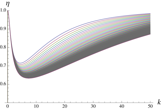
Figure 1: Transmissivity $\eta$ vs. momentum $k$ for $\epsilon$ ranging from $10$ (top curve) to $100$ (bottom curve) by step $1$. The values of other parameters are $\rho=100$ and $m=1$.

3 Information trade-offs for the amplitude damping channel

In the above development, observe that the region for which $\eta$ falls below one is the most important for information storage. In fact, in order to save energy, one would like to have the momentum $k$ as low as possible. However, it is unreasonable to freeze particles such that $k=0$. Hence, we have to face up with the problem of non-negligible information damping, and this motivates us to consider the best strategy for preserving it.

In particular, we would like to preserve both classical and quantum information in the RW spacetime, and so we consider trade-off strategies for doing so [9, 26], modeling the noise as an amplitude damping channel (as motivated in the previous section). To do so, we can model this problem in a communication-theoretic language, in which we say that the device encoding information at the beginning of the evolution is the “sender” and the device recovering information at the end of the evolution is the “receiver.”

A simple strategy for trading between classical and quantum communication is known as time sharing—in a time-sharing strategy, the sender and receiver use a classical communication code for a fraction of the channel uses, a quantum communication code for another fraction, etc. For some channels such as the quantum erasure channel [13], time sharing is an optimal communication strategy, but in general, it cannot outperform a more general strategy known as “trade-off coding” [26]. This allows for transmitting classical and quantum information at net rates $(C,Q)$ that lie in a two-dimensional capacity region.

To proceed with our development for the amplitude damping channel, we begin by recalling that the trade-off region between classical and quantum communication (without the help of entanglement assistance) for any quantum channel $\mathcal{A}_{A^{\prime}\rightarrow B}$ is given by [9]:

$$Q \leq I\left(A\rangle BX\right)_{\rho},$$ (17)

$$C+Q \leq I\left(X;B\right)_{\rho}+I\left(A\rangle BX\right)_{\rho},$$ (18)

where $I(AX;B)_{\rho}\equiv H(AX)_{\rho}+H(B)_{\rho}-H(ABX)_{\rho}$, $I(A\rangle BX)\equiv H(BX)_{\rho}-H(ABX)_{\rho}$, and $I(X;B)_{\rho}\equiv H(X)_{\rho}+H(B)_{\rho}-H(BX)_{\rho}$ denote the quantum mutual information, coherent information, and Holevo information of a quantum state $\rho_{XAB}$, respectively, with the von Neumann entropies defined as $H(A)_{\rho}\equiv-\rm{Tr}\{\rho_{A}\log\rho_{A}\}$, $H(B)_{\rho}\equiv-\rm{Tr}\{\rho_{B}\log\rho_{B}\}$, $H(AB)_{\rho}\equiv-\rm{Tr}\{\rho_{AB}\log\rho_{AB}\}$, etc. (see Chapter 11 of [25], for example, for more on these definitions). These entropies are actually with respect to a classical-quantum state of the following form:

$$\rho_{XAB}\equiv\sum_{x}p_{X}\left(x\right)\left|x\right\rangle\left\langle x\right|_{X}\otimes\mathcal{A}_{A^{\prime}\rightarrow B}\left(|\phi^{x}\rangle_{AA^{\prime}}\langle\phi^{x}|\right),$$ (19)

with $|\phi^{x}\rangle_{AA^{\prime}}\langle\phi^{x}|$ a purification of the input state $\rho_{A^{\prime}}^{x}$ corresponding to the letter $x$. Taking the union of the region specified by (32)-(34) over all ensembles of the form $\left\{p_{X}\left(x\right),|\phi^{x}\rangle_{AA^{\prime}}\langle\phi^{x}|\right\}$ then gives what is known as the single-letter triple trade-off region (meaning that the formulas are a function of a single instance of the channel). We should clarify that the above rate region is an achievable rate region, and for some channels, it is known to be optimal as well [5, 26]. The above rate region is not known to be optimal for the amplitude damping channel.

For the amplitude damping channel $\mathcal{A}$, and hence for the channel (11), we have the following characterization of the single-letter trade-off region:

Theorem 1

The single-letter trade-off region (17)-(18) for the qubit amplitude damping channel is the union of the following polyhedra over all $p_{0},q_{x},\nu_{x}\in\left[0,1\right]$ for $x\in\{0,1\}$ and where $p_{1}=1-p_{0}$ and $p\equiv\sum_{x\in\{0,1\}}p_{x}q_{x}$:

$$Q \leq\sum_{x\in\{0,1\}}p_{x}\,[{\sf g}\left(q_{x},\eta,\nu_{x}\right)-{\sf g}\left(q_{x},1-\eta,\nu_{x}\right)],$$

$$C+Q \leq h_{2}\left(\eta p\right)-\sum_{x\in\{0,1\}}p_{x}\,{\sf g}\left(q_{x},1-\eta,\nu_{x}\right).$$

Furthermore

$${\sf g}\left(q,z,\nu\right)\equiv h_{2}\left(\frac{1+\sqrt{\left(1-2zq\right)^{2}+4z\nu^{2}q(1-q)}}{2}\right),$$

with $h_{2}$ denoting the binary Shannon entropy: $h_{2}(y)\equiv-y\log_{2}y-(1-y)\log_{2}(1-y)$, $y\in[0,1]$.

The proof of Theorem 1 is given in A. We can significantly simplify the characterization of the region when $\eta\geq 1/2$, which is the case of most interest for the physical setting of this paper.

Theorem 2

The single-letter trade-off region (17)-(18) for the qubit amplitude damping channel when $\eta\geq 1/2$ is the union of the following polyhedra over all $p,\nu\in\left[0,1\right]$:

$$Q \leq{\sf g}\left(p,\eta,\nu\right)-{\sf g}\left(p,1-\eta,\nu\right),$$

$$C+Q \leq h_{2}\left(\eta p\right)-{\sf g}\left(p,1-\eta,\nu\right),$$

where ${\sf g}\left(p,z,\nu\right)$ is defined in Theorem 1 and it can be achieved with the following ensemble

$$\frac{1}{2}\left|0\right\rangle\left\langle 0\right|_{X}\otimes\left(\begin{array}[]{cc}1-p&\nu\sqrt{p\left(1-p\right)}\\ \nu\sqrt{p\left(1-p\right)}&p\end{array}\right)_{A^{\prime}}$$ (22)

$$+\frac{1}{2}\left|1\right\rangle\left\langle 1\right|_{X}\otimes\left(\begin{array}[]{cc}1-p&-\nu\sqrt{p\left(1-p\right)}\\ -\nu\sqrt{p\left(1-p\right)}&p\end{array}\right)_{A^{\prime}},$$ (25)

with $p,\nu\in\left[0,1\right]$.

The proof of Theorem 2 is given in B.

Notice that the ensemble that attains the trade-off interpolates between the strategy that achieves the quantum capacity of the amplitude damping channel and that which achieves the product-state classical capacity of the amplitude damping channel, as $\nu$ varies from zero to one. That is, when $\nu=1$, the ensemble reduces to

$$\frac{1}{2}\left|0\right\rangle\left\langle 0\right|_{X}\otimes\left(\begin{array}[]{cc}1-p&\sqrt{p\left(1-p\right)}\\ \sqrt{p\left(1-p\right)}&p\end{array}\right)_{A^{\prime}}$$ (28)

$$+\frac{1}{2}\left|1\right\rangle\left\langle 1\right|_{X}\otimes\left(\begin{array}[]{cc}1-p&-\sqrt{p\left(1-p\right)}\\ -\sqrt{p\left(1-p\right)}&p\end{array}\right)_{A^{\prime}},$$ (31)

which has been proved to be optimal for the product-state classical capacity (the single-letter classical capacity) [12]. When $\nu=0$, the ensemble reduces to

$$\left(\frac{1}{2}\left|0\right\rangle\left\langle 0\right|_{X}+\frac{1}{2}\left|1\right\rangle\left\langle 1\right|_{X}\right)\otimes\left(\begin{array}[]{cc}1-p&0\\ 0&p\end{array}\right)_{A^{\prime}},$$

which is of the diagonal form that achieves the quantum capacity of the amplitude damping channel [12]. The communication strategy resulting from the state in (59) is very different from a naive time-sharing one and outperforms it (see Figure 2).

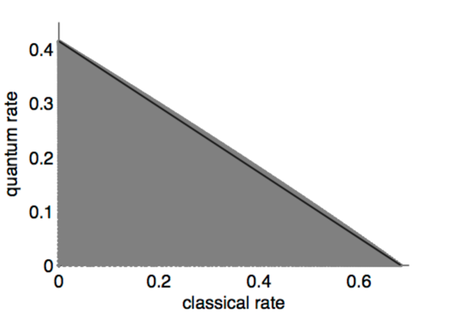
Figure 2: A comparison of a trade-off coding strategy (blue points) versus a time-sharing strategy (red line) for an amplitude damping channel with transmissivity $\eta=0.75$. The figure demonstrates that an ensemble of the form in Theorem 2 outperforms a naive time-sharing strategy between the product-state classical capacity and the quantum capacity.

4 Discussions and Conclusions

In this paper, we have investigated how well information stored in the remote past is preserved when going to the far future, by assuming evolution of the universe in a Robertson-Walker spacetime. We proved, under certain assumptions, that the noise imparted to spin-$\frac{1}{2}$ particles by the evolution of the universe is equivalent to an amplitude damping channel, and we then determined achievable rates for the simultaneous communication of classical and quantum information over this channel. Actually we have established an achievable rate region (and the ensemble to attain it) characterizing communication trade-offs for the qubit amplitude damping channel, thus also generalizing the results given in Ref. [12]. Our results refer to single-letter rate regions, so that it remains open to determine whether a multi-letter characterization could achieve strictly higher rates of communication. For this purpose, one might consider recent approaches developed in [7].

A more physically relevant scenario is the $3+1$ dimensional spacetime with the same evolutionary model adopted here. In this situation spin degrees of freedom of the quantum field become relevant, making physics somehow more involved but richer. An extension of our study to this case is foreseeable thanks to the Bogolyubov transformations given in Ref.[10]. Still we are supposing that the in and out regions spacetime admits natural particle states and a privileged quantum vacuum. If we would employ a more realistic evolutionary model with no static in or out regions, an approximate definition of particles can be made by selecting those mode solutions of the field equation that come in some sense “closest” to Minkowski space limit. Physically this might be envisaged as a construction that ‘ ‘least disturbs” the field by the expansion and in turn leads to the concept of “adiabatic states” (introduced for the scalar fields long time ago [23], then put on rigorous mathematical footing [17] and later on extended to Dirac fields [16]).

In future work, one could also cope with the degradation of the stored information by intervening from time to time and actively correcting the contents of the memory during the evolution of the universe. In this direction, channel capacities taking into account this possibility have been introduced in [21]. In another direction, and much more speculatively, one might attempt to find a meaningful notion for entanglement-assisted communication in our physical scenario by considering Einstein-Rosen bridges along the lines of [18] or entanglement between different universe’s eras, related to dark energy [8].

Acknowledgments

RP would like to thank Jonathan P. Dowling and the Hearne Institute for Theoretical Physics, Louisiana State University, for the kind hospitality. RP and SM are grateful to Shahpoor Moradi for helpful discussions at the early stage of this work. MMW acknowledges support from the Department of Physics and Astronomy at Louisiana State University, from the DARPA Quiness Program through US Army Research Office award W31P4Q-12-1-0019, and from the NSF under Award No. CCF-1350397.

Appendix A Proof of Theorem 1

The two dimensional trade-off region of Theorem 1 is a special case of a theorem determining the triple trade-off region where in addition to $C$ and $Q$ also the net rate $E$ of entanglement consuption/generation is considered.

First we recall that the triple trade-off region for any quantum channel $\mathcal{A}_{A^{\prime}\rightarrow B}$ is given by a union of polyhedra, each of which is specified by the following formulas [25, 26]:

$$C+2Q \leq I\left(AX;B\right)_{\rho},$$ (32)

$$Q+E \leq I\left(A\rangle BX\right)_{\rho},$$ (33)

$$C+Q+E \leq I\left(X;B\right)_{\rho}+I\left(A\rangle BX\right)_{\rho}.$$ (34)

Theorem 3

The single-letter triple trade-off region (32)-(34) for the qubit amplitude damping channel is the union of the following polyhedra over all $p_{0},q_{x},\nu_{x}\in\left[0,1\right]$ for $x\in\{0,1\}$ and where $p_{1}=1-p_{0}$ and $p\equiv\sum_{x\in\{0,1\}}p_{x}q_{x}$:

$$C+2Q \leq h_{2}\left(\eta p\right)+\sum_{x\in\{0,1\}}p_{x}\,[{\sf g}\left(q_{x},1,\nu_{x}\right)-{\sf g}\left(q_{x},1-\eta,\nu_{x}\right)],$$

$$Q+E \leq\sum_{x\in\{0,1\}}p_{x}\,[{\sf g}\left(q_{x},\eta,\nu_{x}\right)-{\sf g}\left(q_{x},1-\eta,\nu_{x}\right)],$$

$$C+Q+E \leq h_{2}\left(\eta p\right)-\sum_{x\in\{0,1\}}p_{x}\,{\sf g}\left(q_{x},1-\eta,\nu_{x}\right),$$

where

$${\sf g}\left(q,z,\nu\right)\equiv h_{2}\left(\frac{1+\sqrt{\left(1-2zq\right)^{2}+4z\nu^{2}q(1-q)}}{2}\right).$$

Proof. From Refs. [25, 26] we have that the so-called “quantum dynamic capacity formula” characterizes the optimization task set out in (32)-(34) (i.e., the task of computing the boundary of the region specified by (32)-(34)). That is, we should optimize the quantum dynamic capacity formula for all non-negative values of the Lagrange multipliers $\lambda$ and $\mu$ and doing so allows us to simplify the form of ensembles necessary to consider in the computation of the boundary of the region. The quantum dynamic capacity formula is given by

$$\max_{\left\{p_{X}\left(x\right),\rho^{x}\right\}}\left(I\left(AX;B\right)_{\rho}+\lambda I\left(A\rangle BX\right)_{\rho}+\mu\left[I\left(X;B\right)_{\rho}+I\left(A\rangle BX\right)_{\rho}\right]\right),$$

(35)

with the entropies referring to the state of (19). As detailed in [25, 26], this is equivalent to

$$I\left(AX;B\right)_{\rho}+\lambda I\left(A\rangle BX\right)_{\rho}+\mu\left[I\left(X;B\right)_{\rho}+I\left(A\rangle BX\right)_{\rho}\right]$$

$$=(1+\mu)H(B)_{\rho}+H(A|X)_{\rho}+\lambda H(B|X)_{\rho}-(1+\mu+\lambda)H(E|X)_{\rho},$$ (36)

where the various von Neumann entropies $H$ can be specified as follows.

A general input qubit density operator for the system $A^{\prime}$ has a matrix representation as follows:

$$\rho^{x}=\left(\begin{array}[]{cc}\langle 1|\rho^{x}|1\rangle&\langle 1|\rho^{x}|0\rangle\\ \langle 0|\rho^{x}|1\rangle&\langle 0|\rho^{x}|0\rangle\end{array}\right)=\left(\begin{array}[]{cc}1-q_{x}&\gamma_{x}\\ \gamma_{x}^{\ast}&q_{x}\end{array}\right),$$ (37)

where $q_{x}\in[0,1]$ and $\gamma_{x}\in\left[0,\sqrt{q_{x}-q_{x}^{2}}\right]$. Sending the qubit density operator (37) through the amplitude damping channel $\mathcal{A}$ of (13) leads to the following state at the output:

$$\mathcal{A}\left(\rho^{x}\right)=\left(\begin{array}[]{cc}1-\eta q_{x}&\sqrt{\eta}\gamma_{x}\\ \sqrt{\eta}\gamma_{x}^{\ast}&\eta q_{x}\end{array}\right).$$ (38)

Then, referring to the state in (19), the output entropy $H(B)$ is

$$H\left(\sum_{x}p_{X}(x)\mathcal{A}(\rho^{x})\right),$$

while the conditional entropy $H\left(A|X\right)$ is

$$\sum_{x}p_{X}\left(x\right)h_{2}\left(\frac{1+\sqrt{\left(1-2q_{x}\right)^{2}+4\left|\gamma_{x}\right|^{2}}}{2}\right).$$ (39)

Furthermore, the conditional entropy $H\left(B|X\right)$ (of the output given which state is input) is as follows:

$$\sum_{x}p_{X}\left(x\right)h_{2}\left(\frac{1+\sqrt{\left(1-2\eta q_{x}\right)^{2}+4\eta\left|\gamma_{x}\right|^{2}}}{2}\right).$$ (40)

On the other hand, sending the qubit density operator in (37) through the channel $\tilde{\mathcal{A}}$ complementary to the amplitude damping channel $\mathcal{A}$ leads to the following state at the environment:

$$\tilde{\mathcal{A}}\left(\rho^{x}\right)=\left(\begin{array}[]{cc}1-\left(1-\eta\right)q_{x}&\sqrt{1-\eta}\gamma_{x}\\ \sqrt{1-\eta}\gamma_{x}^{\ast}&\left(1-\eta\right)q_{x}\end{array}\right).$$ (41)

Then, the conditional entropy $H\left(E|X\right)$ (of the environment given which state is input) is

$$\sum_{x}p_{X}(x)h_{2}\left(\frac{1+\sqrt{\left(1-2\left(1-\eta\right)q_{x}\right)^{2}+4\left(1-\eta\right)\left|\gamma_{x}\right|^{2}}}{2}\right).$$ (42)

As discussed in Refs. [26, 25], any simplification of the quantum dynamic capacity formula can be helpful in reducing the space of parameters over which we need to optimize. So our first aim is to simplify this formula for the case of the amplitude damping channel. To this end we can always augment an ensemble $\rho$ of the form in (19) to become

$$\sum_{x,j}\frac{1}{2}p_{X}\left(x\right)\left|x\right\rangle\left\langle x\right|_{X}\otimes\left|j\right\rangle\left\langle j\right|_{J}\otimes\left(Z^{j}\rho^{x}Z^{j}\right)_{A^{\prime}},$$ (43)

where $Z$ is the Pauli $Z$ operator. This augmentation can only increase communication rates due to the covariance of the amplitude damping channel with respect to $\left\{I,Z\right\}$. Let $\sigma_{XJABE}$ denote the corresponding classical-quantum state that results from purifying each state in the $A^{\prime}$ system and then sending the $A^{\prime}$ system through an isometric extension of the channel. That is,

$$\sigma_{XJABE}\equiv\sum_{x,j}\frac{1}{2}p_{X}\left(x\right)\left|x\right\rangle\left\langle x\right|_{X}\otimes\left|j\right\rangle\left\langle j\right|_{J}\otimes\mathcal{U}_{A^{\prime}\rightarrow BE}^{\mathcal{A}}\left(Z^{j}|\phi^{x}\rangle_{AA^{\prime}}\langle\phi^{x}|Z^{j}\right),$$

with $\mathcal{U}_{A^{\prime}\rightarrow BE}^{\mathcal{N}}$ an isometric extension of the channel $\mathcal{A}_{A^{\prime}\rightarrow B}$. We then have an upper bound for the r.h.s. of (36), namely

$$\!\!\!\!\!\!(1+\mu)H(B)_{\rho}+H(A|X)_{\rho}+\lambda H(B|X)_{\rho}-(1+\mu+\lambda)H(E|X)_{\rho}$$

$$=(1+\mu)H(B)_{\rho}+H(A|XJ)_{\sigma}+\lambda H(B|XJ)_{\sigma}-(1+\mu+\lambda)H(E|XJ)_{\sigma}$$

$$\leq(1+\mu)h_{2}(\eta p)+H(A|XJ)_{\sigma}+\lambda H(B|XJ)_{\sigma}-(1+\mu+\lambda)H(E|XJ)_{\sigma}$$

$$=(1+\mu)h_{2}(\eta p)+\sum_{x}p_{X}\left(x\right)\Bigg{[}h_{2}\left(\frac{1+\sqrt{\left(1-2q_{x}\right)^{2}+4\left|\gamma_{x}\right|^{2}}}{2}\right)$$

$$\ \ \ \ \ \ \ \ \ \ +\lambda h_{2}\left(\frac{1+\sqrt{\left(1-2\eta q_{x}\right)^{2}+4\eta\left|\gamma_{x}\right|^{2}}}{2}\right)$$

$$\ \ \ \ \ \ \ \ \ \ -\left(1+\mu+\lambda\right)h_{2}\left(\frac{1+\sqrt{\left(1-2\left(1-\eta\right)q_{x}\right)^{2}+4\left(1-\eta\right)\left|\gamma_{x}\right|^{2}}}{2}\right)\Bigg{]},$$

where the inequality follows from concavity of entropy and defining

$$p\equiv\sum_{x}p_{X}\left(x\right)q_{x}.$$ (46)

Other steps follow from the covariance of the amplitude damping channel with respect to $I$ and $Z$ operations.

As a consequence of (A), we see that to compute (35), it suffices to optimize the following function of $\left\{\left(p_{X}\left(x\right),q_{x},\gamma_{x}\right)\right\}$ for fixed values of $\lambda$ and $\mu$:

$$\left(1+\mu\right)h_{2}\left(\eta p\right)+\sum_{x}p_{X}\left(x\right)\Bigg{[}h_{2}\left(\frac{1+\sqrt{\left(1-2q_{x}\right)^{2}+4\left|\gamma_{x}\right|^{2}}}{2}\right)$$

$$\hskip 56.9055pt+\lambda h_{2}\left(\frac{1+\sqrt{\left(1-2\eta q_{x}\right)^{2}+4\eta\left|\gamma_{x}\right|^{2}}}{2}\right)$$

$$\hskip 28.45274pt-\left(1+\mu+\lambda\right)h_{2}\left(\frac{1+\sqrt{\left(1-2\left(1-\eta\right)q_{x}\right)^{2}+4\left(1-\eta\right)\left|\gamma_{x}\right|^{2}}}{2}\right)\Bigg{]}.$$

(47)

Clearly, it suffices to take $\gamma_{x}$ real because the above function depends only on the magnitude of $\gamma_{x}$.

First we argue that it is not necessary to consider distributions $p_{X}\left(x\right)$ over more than two letters, and in order to do so, we can apply the Fenchel-Eggelston-Carathéodory theorem often used in the information theory literature for such purposes [11]. That is, we will show that to every probability distribution $p_{X}\left(x\right)$ over an arbitrary number of letters, there exists a probability distribution $p_{X^{\prime}}\left(x^{\prime}\right)$ over just two letters that achieves the same values of the function in (47) for fixed values of $\lambda$ and $\mu$.

Indeed, recall that the Fenchel-Eggelston-Carathéodory theorem states that any point in the convex closure of a connected compact set in $S\subset\mathbb{R}^{d}$ can be represented as a convex combination of at most $d$ points in $S$ (see e.g. [11]). So, let us define the following two functions of the parameters$~{}q$ and$~{}\gamma$:

$$F_{0}\left(q,\gamma\right) \equiv q,$$ (48)

$$F_{1}(q,\gamma) \equiv h_{2}\left(\frac{1+f_{0}(q,\gamma)}{2}\right)+\lambda h_{2}\left(\frac{1+f_{1}(q,\gamma)}{2}\right)$$ (49)

$$-(1+\lambda+\mu)h_{2}\left(\frac{1+f_{2}(q,\gamma)}{2}\right),$$

with

$$f_{0}(q,\gamma)\equiv \sqrt{(1-2q)^{2}+4\gamma^{2}},$$ (50)

$$f_{1}(q,\gamma)\equiv \sqrt{(1-2\eta q)^{2}+4\eta\gamma^{2}},$$ (51)

$$f_{2}(q,\gamma)\equiv \sqrt{(1-2(1-\eta)q)^{2}+4(1-\eta)\gamma^{2}}.$$ (52)

The functions $F_{0}$ and $F_{1}$ are continuous in $q$ and $\gamma$, and the intervals $q\in\left[0,1\right]$ and $\gamma\in\left[0,\sqrt{q-q^{2}}\right]$ are connected and compact, so that the images of these functions are connected and compact as well (the images taken together being in $\mathbb{R}^{2}$). Thus, by applying the Fenchel-Eggelston-Carathéodory theorem, we can conclude that there exists a probability distribution $p_{X^{\prime}}\left(x^{\prime}\right)$ over just two letters such that for $i\in\left\{0,1\right\}$

$$\sum_{x}p_{X}\left(x\right)F_{i}\left(q_{x},\gamma_{x}\right)=\sum_{x^{\prime}}p_{X^{\prime}}\left(x^{\prime}\right)F_{i}\left(q_{x^{\prime}},\gamma_{x^{\prime}}\right).$$ (53)

Finally, the function of interest in (47) is a continuous function of $\sum_{x^{\prime}}p_{X^{\prime}}\left(x^{\prime}\right)F_{i}\left(q_{x^{\prime}},\gamma_{x^{\prime}}\right)$ for $i\in\left\{0,1\right\}$ so that we can conclude that a probability distribution on just two letters suffices for the optimization.

This concludes the proof of Theorem 3 and in turn of Theorem 1. $\hfill\blacksquare$

Appendix B Proof of Theorem 2

Also Theorem 2 can be seen as a special case of an analogous Theorem involving the triple trade-off region.

Theorem 4

The single-letter triple trade-off region (32)-(34) for the qubit amplitude damping channel when $\eta\geq 1/2$ is the union of the following polyhedra over all $p,\nu\in\left[0,1\right]$:

$$C+2Q \leq h_{2}\left(\eta p\right)+{\sf g}\left(p,1,\nu\right)-{\sf g}\left(p,1-\eta,\nu\right),$$

$$Q+E \leq{\sf g}\left(p,\eta,\nu\right)-{\sf g}\left(p,1-\eta,\nu\right),$$

$$C+Q+E \leq h_{2}\left(\eta p\right)-{\sf g}\left(p,1-\eta,\nu\right),$$

where ${\sf g}\left(p,z,\nu\right)$ is defined in Theorem 1 and it can be achieved with the following ensemble

$$\frac{1}{2}\left|0\right\rangle\left\langle 0\right|_{X}\otimes\left(\begin{array}[]{cc}1-p&\nu\sqrt{p\left(1-p\right)}\\ \nu\sqrt{p\left(1-p\right)}&p\end{array}\right)_{A^{\prime}}$$ (56)

$$+\frac{1}{2}\left|1\right\rangle\left\langle 1\right|_{X}\otimes\left(\begin{array}[]{cc}1-p&-\nu\sqrt{p\left(1-p\right)}\\ -\nu\sqrt{p\left(1-p\right)}&p\end{array}\right)_{A^{\prime}},$$ (59)

with $p,\nu\in\left[0,1\right]$.

To prove Theorem 4 we have to show that ensembles of the following simplified form optimize (47):

$$\frac{1}{2}\left|0\right\rangle\left\langle 0\right|_{X}\otimes\left(\begin{array}[]{cc}1-p&\nu\sqrt{p\left(1-p\right)}\\ \nu\sqrt{p\left(1-p\right)}&p\end{array}\right)_{A^{\prime}}$$ (62)

$$+\frac{1}{2}\left|1\right\rangle\left\langle 1\right|_{X}\otimes\left(\begin{array}[]{cc}1-p&-\nu\sqrt{p\left(1-p\right)}\\ -\nu\sqrt{p\left(1-p\right)}&p\end{array}\right)_{A^{\prime}}.$$ (65)

This is equivalent to showing that for every $\{p_{X}(x),q_{x}\}_{x\in\{0,1\}}$ such that $\sum_{x}p_{X}(x)q_{x}=p$, there exists a value of $\nu$ such that

$$\sum_{x}p_{X}\left(x\right)\Bigg{[}h_{2}\left(\frac{1+\sqrt{\left(1-2q_{x}\right)^{2}+4\left|\gamma_{x}\right|^{2}}}{2}\right)$$

$$+\lambda h_{2}\left(\frac{1+\sqrt{\left(1-2\eta q_{x}\right)^{2}+4\eta\left|\gamma_{x}\right|^{2}}}{2}\right)$$

$$-\left(1+\mu+\lambda\right)h_{2}\left(\frac{1+\sqrt{\left(1-2\left(1-\eta\right)q_{x}\right)^{2}+4\left(1-\eta\right)\left|\gamma_{x}\right|^{2}}}{2}\right)\Bigg{]}$$

$$\leq h_{2}\left(\frac{1+\sqrt{\left(1-2p\right)^{2}+4\nu^{2}p(1-p)}}{2}\right)$$

$$+\lambda h_{2}\left(\frac{1+\sqrt{\left(1-2\eta p\right)^{2}+4\eta\nu^{2}p(1-p)}}{2}\right)$$

$$-\left(1+\mu+\lambda\right)h_{2}\left(\frac{1+\sqrt{\left(1-2\left(1-\eta\right)p\right)^{2}+4\left(1-\eta\right)\nu^{2}p(1-p)}}{2}\right).$$ (66)

Let us have a closer look at the function $F_{1}$ of Eq.(49). Its first derivative with respect to $\gamma$ is as follows:

$$\ln 2\;\frac{\partial F_{1}(q,\gamma)}{\partial\gamma} =(1+\mu+\lambda)\frac{2(1-\eta)\gamma}{f_{2}}\ln\frac{1+f_{2}}{1-f_{2}}$$ (67)

$$-\lambda\frac{2\eta\gamma}{f_{1}}\ln\frac{1+f_{1}}{1-f_{1}}-\frac{2\gamma}{f_{0}}\ln\frac{1+f_{0}}{1-f_{0}}\,.$$

This is a linear function of $\mu$, hence we can determine a critical value of $\mu$ below (resp. above) which $\frac{\partial F_{1}(q,\gamma)}{\partial\gamma}$ is always negative (resp. positive). It is given by

$$\mu^{\ast}=-(1+\lambda)+\frac{1}{\frac{1-\eta}{f_{2}}\ln\frac{1+f_{2}}{1-f_{2}}}\Bigg{[}\lambda\frac{\eta}{f_{1}}\ln\frac{1+f_{1}}{1-f_{1}}+\frac{1}{f_{0}}\ln\frac{1+f_{0}}{1-f_{0}}\Bigg{]}\,.$$ (68)

The second derivative of $F_{1}$ with respect to $q$, in turn, is equal to

$$\ln 2\;\frac{\partial^{2}F_{1}(q,\gamma)}{\partial q^{2}}=-\frac{4}{f_{0}^{2}}\,\left[\frac{2\gamma^{2}}{f_{0}}\ln{\frac{1+f_{0}}{1-f_{0}}}+\frac{(1-2q)^{2}}{1-f_{0}^{2}}\right]$$

$$-4\,\lambda\,\frac{\eta^{2}}{f_{1}^{2}}\,\left[\frac{2\eta\gamma^{2}}{f_{1}}\ln{\frac{1+f_{1}}{1-f_{1}}}+\frac{(1-2\eta q)^{2}}{1-f_{1}^{2}}\right]$$

$$+4\,(1+\mu+\lambda)\frac{(1-\eta)^{2}}{f_{2}^{2}}\left[\frac{2(1-\eta)\gamma^{2}}{f_{2}}\ln{\frac{1+f_{2}}{1-f_{2}}}+\frac{(1-2(1-\eta)q)^{2}}{1-f_{2}^{2}}\right].$$

This is also a linear function of $\mu$, and there exists a critical value of $\mu$ below (resp. above) which $\frac{\partial^{2}F_{1}(q,\gamma)}{\partial q^{2}}$ is always negative (resp. positive). It is given by

$$\mu^{\ast\ast}=-(1+\lambda) +\frac{\frac{f_{2}^{2}}{(1-\eta)^{2}}}{\frac{{1-\eta}}{f_{2}}\ln\frac{1+f_{2}}{1-f_{2}}+\frac{f_{2}^{2}-4(1-\eta)\gamma^{2}}{2\gamma^{2}(1-f_{2}^{2})}}\Bigg{[}\lambda\frac{\eta^{3}}{f_{1}^{3}}\ln\frac{1+f_{1}}{1-f_{1}}+\frac{1}{f_{0}^{3}}\ln\frac{1+f_{0}}{1-f_{0}}$$ (69)

$$+\lambda\frac{\eta^{2}}{2\gamma^{2}f_{1}^{2}}\frac{f_{1}^{2}-4\eta\gamma^{2}}{1-f_{1}^{2}}+\frac{1}{2\gamma^{2}{f_{0}^{2}}}\frac{f_{0}^{2}-4\gamma^{2}}{(1-f_{0}^{2})}\Bigg{]}.$$

By inspection, it follows that $\mu^{\ast}\leq\mu^{\ast\ast}$ for $\eta\geq\frac{1}{2}$ (for $\eta<\frac{1}{2}$ one can always find a large enough value of $\lambda$ that invalidate the condition). Anyway this is the only relevant regime for our purposes since for $\eta<\frac{1}{2}$ the quantum capacity of the amplitude damping channel vanishes. Let us then distinguish the following two situations:

B.1 $\mu\leq\mu^{\ast\ast}$, i.e. $F_{1}$ is concave with respect to $q$

In this case $F_{1}$ is a monotonic function of $\gamma$. It is decreasing with increasing $\gamma$ for $\mu\leq\mu^{\ast}\leq\mu^{\ast\ast}$ and increasing with increasing $\gamma$ for $\mu^{\ast}\leq\mu\leq\mu^{\ast\ast}$.

Nevertheless (remembering that it suffices to consider two letters) if we take two arbitrary points $(q_{0},\gamma_{0})$ and $(q_{1},\gamma_{1})$ in the $q,\gamma$ plane and suppose w.l.g. that $\gamma_{1}>\gamma_{0}$, we have

$$F_{1}(q_{1},\gamma_{1}) \leq F_{1}(q_{1},\gamma_{0}),\qquad(F_{1}\;\mathrm{decreasing\;vs}\;\gamma),$$

$$F_{1}(q_{1},\gamma_{1}) \geq F_{1}(q_{1},\gamma_{0}),\qquad(F_{1}\;\mathrm{increasing\;vs}\;\gamma),$$

hence

$$p_{0}F_{1}(q_{0},\gamma_{0})+p_{1}F_{1}(q_{1},\gamma_{1})\leq p_{0}F_{1}(q_{0},\gamma_{0})+p_{1}F_{1}(q_{1},\gamma_{0}),$$

$$(F_{1}\;\mathrm{decreasing\;vs}\;\gamma),$$

$$p_{0}F_{1}(q_{0},\gamma_{0})+p_{1}F_{1}(q_{1},\gamma_{1})\leq p_{0}F_{1}(q_{0},\gamma_{1})+p_{1}F_{1}(q_{1},\gamma_{1}),$$

$$(F_{1}\;\mathrm{increasing\;vs}\;\gamma).$$

However, by the concavity of $F_{1}$ with respect to $q$ we can further write

$$p_{0}F_{1}(q_{0},\gamma_{0})+p_{1}F_{1}(q_{1},\gamma_{1})\leq F_{1}(p_{0}q_{0}+p_{1}q_{1},\gamma_{0}),$$ (70)

$$(F_{1}\;\mathrm{decreasing\;vs}\;\gamma),$$

$$p_{0}F_{1}(q_{0},\gamma_{0})+p_{1}F_{1}(q_{1},\gamma_{1})\leq F_{1}(p_{0}q_{0}+p_{1}q_{1},\gamma_{1}),$$ (71)

$$(F_{1}\;\mathrm{increasing\;vs}\;\gamma).$$

So this proves (66) for this case. Notice that when $F_{1}$ is a decreasing function of $\gamma$ the optimal value of $\gamma$ is $0$, while when $F_{1}$ is an increasing function of $\gamma$ the optimal value of $\gamma$ is the maximum allowed one, i.e. $\sqrt{q-q^{2}}$.

B.2 $\mu\geq\mu^{\ast\ast}$, i.e. $F_{1}$ is convex with respect to $q$

In this case $F_{1}$ is a monotonic increasing function of $\gamma$. Hence, we should look for a suitable value of $\gamma$, say $\tilde{\gamma}$, such that the following inequality (equivalent to (66))

$$p_{0}F_{1}(q_{0},\gamma_{0})+p_{1}F_{1}(q_{1},\gamma_{1})\leq F_{1}(p_{0}q_{0}+p_{1}q_{1},\tilde{\gamma}),$$ (72)

is satisfied for any arbitrary points $(q_{0},\gamma_{0})$ and $(q_{1},\gamma_{1})$ in the $q,\gamma$ plane (again remembering that it suffices to consider two letters).

Since $F_{1}$ becomes increasingly convex with increasing $\mu$, the worst situation is represented by the limit as $\mu\to\infty$, where

$$F_{1}(q,\gamma)\approx-\mu\,h_{2}\left(\frac{1+f_{2}(q,\gamma)}{2}\right).$$ (73)

To be on the safe side, let us consider $\gamma_{0}=\gamma_{1}=0$ where the difference between the chord on the l.h.s. of (72) and the function $F_{1}(p_{0}q_{0}+p_{1}q_{1},0)$ is maximum. There, the worst situation is represented by $q_{0}=0$, $q_{1}=1$ (hence $q=p_{1}$), for which we have

$$(1-q)F_{1}(0,0)+qF_{1}(1,0)\leq F_{1}(q,\tilde{\gamma}).$$ (74)

Taking $\tilde{\gamma}=\sqrt{q-q^{2}}$ and accounting for (73) this gives

$$q\mu\,h_{2}\left(1-(1-\eta)q\right)\geq 0,$$ (75)

which always holds true.

This concludes the proof of Theorem 4 and in turn of Theorem 2. $\hfill\blacksquare$

As consequence of Theorem 4, also the communication strategy involving entanglement results quite different from a naive time-sharing one and outperforms it (see Figure 3).

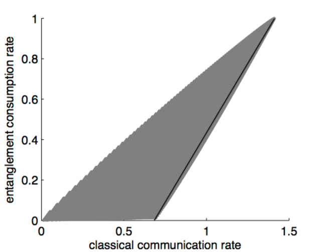
Figure 3: A comparison of a trade-off coding strategy (blue points) versus a time-sharing strategy (red line) for an amplitude damping channel with transmissivity $\eta=0.75$. The figure demonstrates that an ensemble of the form in Theorem 4 outperforms a naive time-sharing strategy between the product-state classical capacity and the entanglement-assisted classical capacity.

References

References

• [1] N. D. Birrell and P. C. W. Davies, Quantum fields in curved space, Cambridge University Press (1984).
• [2] K. Brádler, P. Hayden and P. Panangaden, Journal of High Energy Physics 8, 74 (2009).
• [3] K. Brádler and C. Adami, arXiv:1310.7914 (2013)
• [4] K. Brádler, P. Hayden and P. Panangaden, Communications in Mathematical Physics 312, 361 (2012).
• [5] K. Brádler, P. Hayden, D. Touchette and M. M. Wilde, Physical Review A 81, 062312 (2010).
• [6] K. Brádler, T. J. O’Connor and R. Jauregui, Journal of Mathematical Physics 52, 062202 (2011).
• [7] F. G. S. L. Brandao, J. Eisert, M. Horodecki and D. Yang, Physical Review Letters 106, 230502 (2011).
• [8] S. Capozziello, O. Luongo and S. Mancini, Physics Letters A 377 1061 (2013).
• [9] I. Devetak and P. W. Shor, Communications in Mathematical Physics, 256, 287 (2005).
• [10] A. Duncan, Physical Review D 17, 964 (1978).
• [11] A. El Gamal and Y.H. Kim, Network information theory, Cambridge University Press (2012).
• [12] V. Giovannetti and R. Fazio, Physical Review A 71, 032314 (2005).
• [13] M. Grassl, T. Beth and T. Pellizzari, Physical Review A 56, 33 (1997).
• [14] S. W. Hawking, Communications in Mathematical Physics 43, 199 (1975).
• [15] P. Hayden and J. Preskill, Journal of High Energy Physics, 9, 120 (2007).
• [16] S. Hollands, Communications in Mathematical Physics 216, 635 (2001).
• [17] C. Luders and J. E. Roberts, Communications in Mathematical Physics 134, 29 (1990).
• [18] J. Maldacena and L. Susskind. arXiv:1306.0533 (2013).
• [19] E. Martin-Martinez, D. Hosler and M. Montero, Physical Review A 86, 62307 (2012).
• [20] S. Moradi, R. Pierini and S. Mancini, Physical Review D 89, 024022 (2014).
• [21] A. Muller-Hermes, D. Reeb and M. M. Wolf, arXiv:1310.2856 (2013).
• [22] T. J. O’Connor, K. Bradler and M. M. Wilde, Journal of Physics A 44, 415306 (2011).
• [23] L. Parker, Physical Review 183, 1057 (1969).
• [24] R. M. Wald, Quantum fields theory in curved space time and black holes thermodynamics, The University of Chicago Press (1994).
• [25] M. M. Wilde, Quantum Information Theory, Cambridge University Press (2013).
• [26] M. M. Wilde and M.-H. Hsieh, Quantum Information Processing 11, 1431 (2012).