Is the effect of the Sun’s gravitational potential on dark matter particles observable?

Abstract

We consider the effect of the Sun’s gravitational potential on the local phase space distribution of dark matter particles, focusing on its implication for the annual modulation signal in direct detection experiments. We perform a fit to the modulation signal observed in DAMA/LIBRA and show that the allowed region shrinks if Solar gravitational focusing (GF) is included compared to the one without GF. Furthermore, we consider a possible signal in a generic future direct detection experiment, irrespective of the DAMA/LIBRA signal. Even for scattering cross sections close to the current bound and a large exposure of a xenon target with 270 ton yr it will be hard to establish the presence of GF from data. In the region of dark matter masses below 40 GeV an annual modulation signal can be established for our assumed experimental setup, however GF is negligible for low masses. In the high mass region, where GF is more important, the significance of annual modulation itself is very low. We obtain similar results for lighter targets such as Ge and Ar. We comment also on inelastic scattering, noting that GF becomes somewhat more important for exothermic scattering compared to the elastic case.

1 Introduction

The effect of the Sun’s gravitational potential on the local phase space distribution of Galactic dark matter (DM) particles and its effect on DM direct detection experiments have been considered by a number of authors [1, 2, 3], see also [5, 6, 4]. It turns out that the effect on the total scattering rate of DM particles is very small. Recently, in Ref. [7], it was pointed out, however, that Solar gravitational focusing (GF) may have a sizable effect on the phase of the annual modulation in the DM–nucleus scattering rate. Such a modulation is induced by the motion of the Earth around the Sun, while the Sun moves through the Galactic halo [8, 9]. On top of this effect due to boosting the dark matter velocity distribution into the Earth’s rest frame, an additional modulation is induced by the distortion of the DM phase space density through the Sun’s gravitational potential. The boost effect has its minima and maxima around June and December, when the Sun’s and Earth’s velocities add up or subtract. The GF induced modulation will have minima and maxima when the Earth is located behind or in front of the Sun, which happens in March and September, respectively. Hence, the net-modulation will emerge as an interplay of those two effects, which may significantly affect the phase of the signal.

In section 2 below, after fixing the notation, we are going to discuss those effects in terms of the so-called halo integral, which captures the time dependence of the signal in a particle physics as well as experimental configuration independent way. In the following we present numerical studies of this effect, investigating whether GF can be established from data, as well as its impact on extracting DM parameters. As a first case study we consider in section 3 the annual modulation signal reported by the DAMA/LIBRA collaboration [10] and show that taking into account GF leads to a more constrained region in the plane of DM mass and scattering cross section. However, the relevant region in parameter space is highly excluded by data from several other experiments. In particular, the LUX (Large Underground Xenon) experiment [11] has set the strongest limits on the spin-independent elastic WIMP-nucleon cross section, with a minimum upper limit of $7.6\times 10^{-46}$ cm² on the cross section at 90% CL for a DM mass of 33 GeV assuming the Standard Halo Model. Therefore, we proceed in section 4 by discarding the DAMA/LIBRA signal and consider a hypothetical future experiment. To be specific, we assume a large scale liquid xenon experiment, along the lines discussed in [12, 13, 14, 15]. Our results indicate that even with a very large exposure of several 100 ton yr it will be difficult to establish an annual modulation signal at high significance where GF has an observable effect. In subsection 4.4 we comment briefly on light target nuclei. For most part of the work we assume elastic spin-independent scattering; in subsection 4.5 we comment also on inelastic scattering. We summarize in section 5.

2 Annual modulation with gravitational focusing

2.1 Notation

The differential rate in events/keV/kg/day for a dark matter particle $\chi$ to scatter off a nucleus $(A,Z)$ and deposit the nuclear recoil energy $E_{nr}$ in the detector is given by

$${R}(E_{nr},t)=\frac{\rho_{\chi}}{m_{\chi}}\frac{1}{m_{A}}\int_{v>v_{m}}d^{3}v\frac{d\sigma_{A}}{d{E_{nr}}}vf_{\rm det}(\boldsymbol{\rm v},t),$$ (2.1)

where $\rho_{\chi}$ is the local DM density, $m_{A}$ and $m_{\chi}$ are the nucleus and DM masses, $\sigma_{A}$ is the DM–nucleus scattering cross section and $\boldsymbol{\rm v}$ is the 3-vector relative velocity between DM and the nucleus, while $v\equiv|\boldsymbol{\rm v}|$. $f_{\rm det}(\boldsymbol{\rm v},t)$ is the DM velocity distribution in the detector reference frame. For elastic scattering, the minimal velocity $v_{m}$ required for a DM particle to deposit a recoil energy $E_{nr}$ in the detector is given by

$$v_{m}=\sqrt{\frac{m_{A}E_{nr}}{2{\mu_{\chi A}^{2}}}},$$ (2.2)

where $\mu_{\chi A}$ is the reduced mass of the DM–nucleus system.

The time dependence of the differential event rate is due to the velocity of the Earth with respect to the Sun, $\boldsymbol{\rm v}_{e}(t)$, which can be written as [16]

$$\boldsymbol{\rm v}_{e}(t)=v_{e}[\boldsymbol{\rm e}_{1}\sin\lambda(t)-\boldsymbol{\rm e}_{2}\cos\lambda(t)]\,,$$ (2.3)

with $v_{e}=29.8$ km/s, and $\lambda(t)=2\pi(t-0.218)$ with $t$ in units of 1 year and $t=0$ at January 1st, while $\boldsymbol{\rm e}_{1}=(-0.0670,0.4927,-0.8676)$ and $\boldsymbol{\rm e}_{2}=(-0.9931,-0.1170,0.01032)$ are orthogonal unit vectors spanning the plane of the Earth’s orbit. We are using Galactic coordinates where $x$ points towards the Galactic Center, $y$ in the direction of the Galactic rotation, and $z$ towards the Galactic North, perpendicular to the disc. As shown in [17], Eq. (2.3) provides an excellent approximation to describe the annual modulation signal. However, corrections to Eq. (2.3) become relevant for higher harmonics of the time dependence. When discussing bi-annual modulation in section 2.2 we do include the eccentricity of the orbit following Refs. [18, 19].

Including the effect of GF, the DM density times the velocity distribution in Eq. (2.1) is obtained by

$$\rho_{\chi}f_{\rm det}(\textbf{v},t)=\rho_{\infty}\tilde{f}(\textbf{v}_{\odot}+\textbf{v}_{\infty}[\textbf{v}+\textbf{v}_{e}])\,.$$ (2.4)

Here $\rho_{\infty}=0.3$ GeV$/$cm³ and $\tilde{f}(\textbf{v})$ are the DM density and velocity distribution in the Galactic rest frame measured near the Solar System, but far away from the Sun, such that the Sun’s gravitational potential is small, and $\textbf{v}_{\odot}\approx(10,233,7)$ km/s is the velocity of the Sun with respect to the Galaxy. The function $\textbf{v}_{\infty}[\textbf{v}]$ relates the velocity $\textbf{v}_{\infty}$ of a DM particle relative to the Sun far away from the Sun’s gravitational potential to the particle’s velocity v at the detector [3]:

$$\textbf{v}_{\infty}[\textbf{v}]=\frac{v_{\infty}^{2}\textbf{v}+v_{\infty}u_{\rm esc}^{2}\hat{\bf r}_{s}/2-v_{\infty}\textbf{v}(\textbf{v}\cdot\hat{\bf r}_{s})}{v_{\infty}^{2}+u_{\rm esc}^{2}/2-v_{\infty}(\textbf{v}\cdot\hat{\bf r}_{s})}\,,$$ (2.5)

with $v_{\infty}^{2}=v^{2}-u_{\rm esc}^{2}$, where $u_{\rm esc}=\sqrt{2GM_{\odot}/r_{\rm A.U.}}\simeq 40$ km/s is the escape velocity from the Sun near the Earth’s orbit, and is of ${\mathcal{O}}(v_{e})$, while $\hat{\bf r}_{s}$ is the unit vector pointing in the direction of the Earth from the center of the Solar System, and is given by

$$\hat{\bf r}_{s}=-[\boldsymbol{\rm e}_{1}\cos\lambda(t)+\boldsymbol{\rm e}_{2}\sin\lambda(t)]\,.$$ (2.6)

If GF is neglected, the velocity distribution in the detector’s rest frame is obtained just by a boost from the Galactic rest frame: $f_{\rm det}(\textbf{v},t)=\tilde{f}(\textbf{v}+\textbf{v}_{\odot}+\textbf{v}_{e})$ and $\rho_{\chi}=\rho_{\infty}$. In this paper we assume the so-called Standard Halo Model with a truncated Maxwellian velocity distribution,

$$\tilde{f}(\textbf{v})=\frac{1}{N}\left[\exp\left(-\frac{\textbf{v}^{2}}{\bar{v}^{2}}\right)-\exp\left(-\frac{v_{\rm esc}^{2}}{\bar{v}^{2}}\right)\right]\Theta(v_{\rm esc}-v)\,,$$ (2.7)

where $N$ is a normalization constant and we adopt the fiducial values $\bar{v}=220$ km/s and $v_{\rm esc}=544$ km/s.

We focus here on spin-independent elastic scattering and assume that DM couples with the same strength to protons and neutrons. In this case the differential cross section which enters in Eq. (2.1) is

$$\frac{d\sigma_{A}}{dE_{nr}}=\frac{m_{A}A^{2}}{2\mu_{\chi p}^{2}v^{2}}{\sigma_{\rm SI}}F^{2}(E_{nr})\,,$$ (2.8)

where $\sigma_{\rm SI}$ is the spin-independent DM–nucleon scattering cross section, $\mu_{\chi p}$ is the reduced mass of the DM–nucleon system, and $F(E_{nr})$ is a form factor.

Defining the halo integral as

$$\eta(v_{m},t)\equiv\int_{v>v_{m}}d^{3}v\frac{\tilde{f}(\textbf{v}_{\odot}+\textbf{v}_{\infty}[\textbf{v}+\textbf{v}_{e}],t)}{v}\,,$$ (2.9)

the event rate is given by

$$R(E_{nr},t)=C\,F^{2}(E_{nr})\,\eta(v_{m},t),\qquad\text{with}\qquad C=\frac{\rho_{\infty}A^{2}\sigma_{\rm SI}}{2m_{\chi}\mu_{\chi p}^{2}}.$$ (2.10)

The coefficient $C$ contains the particle physics dependence, while $\eta(v_{m},t)$ parametrizes the astrophysics. The number of events in an energy interval $[E_{1},E_{2}]$ and at a given time $t$ can be written as

$$N_{[E_{1},E_{2}]}(t)=MT\int_{0}^{\infty}dE_{nr}G_{[E_{1},E_{2}]}(E_{nr})R(E_{nr},t)\,,$$ (2.11)

where $MT$ is the exposure of the experiment in units of kg day, and $G_{[E_{1},E_{2}]}(E_{nr})$ is the detector response function which includes the detection efficiencies and energy resolution. The response function may be non-zero outside the interval $[E_{1},E_{2}]$ due to the energy resolution. The annual modulation signal in a given energy interval can be computed by subtracting the time averaged events from the total number of events in that energy interval. We have

$$A_{[E_{1},E_{2}]}(t)=\frac{N_{[E_{1},E_{2}]}(t)-\langle N_{[E_{1},E_{2}]}(t)\rangle_{t}}{E_{2}-E_{1}}\,,$$ (2.12)

where $\langle N_{[E_{1},E_{2}]}(t)\rangle_{t}$ is the number of events averaged over one year in the given energy bin. The units are events/keV.

2.2 Time dependence of the halo integral

Let us now discuss the time dependence of the event rate in a direct detection experiment, which according to Eq. (2.10) is determined from the time dependence of the halo integral defined in Eq. (2.9). Note that the time variation of $\eta(v_{m},t)$ is independent of particle physics, in particular independent of the DM mass. Assuming the Maxwellian, Eq. (2.7), we calculate $\eta(v_{m},t)$ numerically. For a fixed minimal velocity $v_{m}$ we perform a Fourier decomposition in $t$. In the left panel of Fig. 1 we compare the size of the amplitude of the first harmonic (annual modulation) as well as the second harmonic (bi-annual modulation) to the time-averaged component (zeroth order Fourier coefficient). The right panel shows the date of the maximum of the first harmonic. In this subsection we do not use Eqs. (2.3) and (2.6) to describe $\boldsymbol{\rm v}_{e}(t)$ and $\hat{\bf r}_{s}(t)$, but instead use the expressions given in the appendix of Ref. [19] (see also [18] for equivalent results) including the eccentricity of the Earth’s orbit. This is relevant for the second harmonic. We have verified that for the first harmonic corrections due to the eccentricity are negligible and Eqs. (2.3) and (2.6) are sufficient.

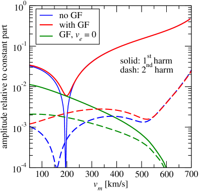
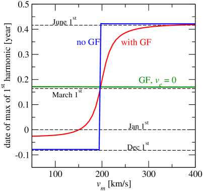
Figure 1: Time variation of the halo integral $\eta(v_{m},t)$ as defined in Eq. (2.9). We assume a Maxwellian velocity distribution and perform a Fourier analysis of $\eta(v_{m},t)$ for fixed minimal velocity $v_{m}$. The left plot shows the amplitudes of the first (solid) and second (dashed) harmonics relative to the time independent component. In the right panel we show the date of the maximum of the first harmonic as a function of $v_{m}$. In both panels we show the cases of neglecting Solar GF (blue), taking GF into account (red), and the effect of GF for setting the Earth’s velocity relative to the Sun to zero (green).

The blue curves in the figure correspond to the traditional case of neglecting GF. The first harmonic shows the characteristic phase flip close to $v_{m}\approx 200$ km/s, where the amplitude goes to zero and below (above) that value of $v_{m}$ the maximum is at the beginning of December (June). The second harmonic without GF has two phase flips [20], one around 150 km/s and another one around 500 km/s. Note that for the second phase flip the amplitude does not go to zero. The reason is related to the effect of the Earth’s orbit eccentricity, which makes the maximum shift smoothly by $\pi/2$ but the amplitude remains non-zero. Once GF is included (red curves) we can make the following observations: $(i)$ the amplitude of the first harmonic is hardly affected by GF, the only exception being close to the phase flip, with the amplitude never going to zero; $(ii)$ there is a significant distortion of the maximum of the first harmonic around and below the phase flip (see right panel). The date of the maximum moves smoothly from around December 20 at very low $v_{m}$ to beginning of June for large $v_{m}$. Those results are in agreement with [7]; and ($iii$) the amplitude of the second harmonic is significantly affected by GF, leading even to the disappearance of the phase flip at low $v_{m}$.

For illustration purpose we show in Fig. 1 also the effect of GF but assuming that the Earth is at rest with respect to the Sun (green curves). This corresponds to the hypothetical situation of considering fixed positions of the Earth in turn and comparing the event rates at the different locations of the Earth around the Sun. This procedure isolates the effect of GF and removes the time dependence from the velocity boost. Technically what we do is to set $v_{e}=0$ but keep the time dependence of $\hat{\bf r}_{s}$ in Eq. (2.5). By comparing the blue and green curves in the left panel we see the relative importance of the time dependence induced by the velocity boost and GF. While for the first harmonic GF is always subdominant (except at the phase flip), for the second harmonic it is dominating for $v_{m}\lesssim 300$ km/s. The right panel shows that the first harmonic induced by GF only (green curve) always peaks at the beginning of March, independent of $v_{m}$.

We do not discuss further the second harmonic, since this will be very hard to observe in the foreseeable future. Focusing on the first harmonic, we conclude that the main effect of GF is the modification of the phase, especially for $v_{m}\lesssim 250$ km/s [7]. In the rest of the paper we will perform numerical studies of the importance (statistical significance) of this effect in (semi)realistic experimental situations.

3 Gravitational focusing and the DAMA/LIBRA signal

The DAMA/LIBRA collaboration [10] reports a highly significant annual modulation signal using an NaI target, which can be interpreted in terms of elastic spin-independent DM scattering with DM masses of around 10 or 80 GeV, depending on whether scattering happens on the sodium or iodine nucleus. Despite the fact that the required cross sections are excluded by a number of other experiments, we consider their data as a case study in order to investigate the effect of GF for extracting DM parameters. Ideally one would perform a fit to the data using time as well as energy information. Unfortunately this information is not public, since data are presented either binned in time or in energy (but not showing the full 2-dimensional information). Since the main effect of GF is a distortion of the time behavior of the signal we are using here time binned data, extracted from the top panel of Fig. 1 in Ref. [10]. This figure shows the time variation of the count rate in the $[2,4]$ keVee energy interval corresponding to a 0.87 ton yr exposure during about 5.5 years divided into 43 bins. In this energy interval, the modulation signal is largest. We use $q_{\rm Na}=0.3$ and $q_{\rm I}=0.09$ for the quenching factors of Na and I, respectively [21], and assume a Gaussian energy resolution with an energy dependent width as presented in Ref. [22].

To fit the DAMA data, we construct a $\chi^{2}$ function

$$\chi^{2}_{\rm DAMA}(m_{\chi},\sigma_{\rm SI})=\sum_{i=1}^{43}\left(\frac{A_{i}^{\rm pred}(m_{\chi},\sigma_{\rm SI})-A_{i}^{\rm obs}}{\sigma_{i}}\right)^{2},$$ (3.1)

where $A_{i}^{\rm obs}$ and $\sigma_{i}$ are the experimental data points and their errors, respectively, from the top panel of Fig. 1 in Ref. [10]. The sum is over the 43 time bins. The best fit point can be found by minimizing Eq. (3.1) with respect to the WIMP mass $m_{\chi}$, and cross section $\sigma_{\rm SI}$. The allowed regions in the mass – cross section plane at a given CL are obtained by looking for contours $\chi^{2}(m_{\chi},\sigma_{\rm SI})=\chi^{2}_{\rm min}+\Delta\chi^{2}({\rm CL})$, where $\Delta\chi^{2}({\rm CL})$ is evaluated for 2 degrees of freedom (dof), e.g., $\Delta\chi^{2}(90\%)=4.6$.

Fig. 2 shows the allowed region of DAMA at 90% CL and 3$\sigma$ in the cross section and mass plane assuming $A_{i}^{\rm pred}$ is with (black contours) or without (dark and light red regions) GF. With GF, $\chi^{2}_{\rm min}=40.6$ for $m_{\chi}=76.9$ GeV and $\sigma_{\rm SI}=1.3\times 10^{-41}$ cm². The minimum is shown with a star in Fig. 2. Without GF, $\chi^{2}_{\rm min}\approx 42.2$ is practically degenerate along the allowed strip in parameter space visible in the figure between DM masses from $\sim 5$ GeV to more than 100 GeV.

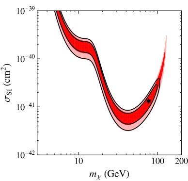
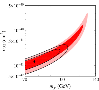
Figure 2: The preferred region of DAMA at 90% CL and 3$\sigma$ with (black contours) and without (dark and light red regions) GF using time binned data in the single energy interval of 2 to 4 keVee. The left panel shows the result for a large range of dark matter masses, while the right panel zooms on the mass region where GF is important. The black star shows the best fit location with GF.

The $\chi^{2}_{\rm min}$ values in both cases are of order of the number of degrees of freedom (43 data points minus 2 fitted parameters), indicating a good fit without as well as with GF. However, one can see from Fig. 2 that GF makes the preferred DAMA region smaller, excluding the region of large DM masses. According to Eq. (2.2), large masses correspond to small values of $v_{m}$, and in this region the phase shift induced by GF becomes relevant, leading to a disagreement with the data. In contrast, the region $\lesssim 80$ GeV is practically unaffected by GF, which holds in particular also for the $m_{\chi}\sim 10$ GeV solution from scattering on sodium. For such light DM masses, $v_{m}$ becomes large and only the high velocity tail of the DM distribution is probed, where GF is negligible, c.f., Fig. 1.

Let us comment on the fact that the allowed region in Fig. 2 appears as a degenerate band, in contrast to the familiar two isolated regions (see [23] for a recent example). As explained above, the fit on which Fig. 2 is based on uses only limited information on the energy dependence of the signal, since it uses time binned data in a single energy interval. However, the energy spectrum is quite powerful to constrain the allowed region [22, 24] and this information is missed in the current analysis. Ideally time and energy information should be included simultaneously. In the absence of this information we present an alternative fit to the DAMA data using information from Fig. 9 of Ref. [10]. There the result of fitting a cosine function to the total exposure (1.17 ton yr, DAMA/NaI and DAMA/LIBRA) is presented, showing in different energy bins the amplitude of the cosine, $Y_{m}$ (upper panel), and the time of the maximum, $t^{*}$ (lower panel). Neglecting a possible correlation between $Y_{m}$ and $t^{*}$ (as justified by Fig. 7 of [10]) we can use this to construct a $\chi^{2}$ function as

$$\chi^{2}_{\rm DAMA^{\prime}}(m_{\chi},\sigma_{\rm SI})=\sum_{i=1}^{7}\left(\frac{Y_{m,i}^{\rm pred}(m_{\chi},\sigma_{\rm SI})-Y_{m,i}^{\rm obs}}{\sigma_{i}^{Y_{m}}}\right)^{2}+\sum_{j=1}^{4}\left(\frac{t_{j}^{*,\rm pred}(m_{\chi},\sigma_{\rm SI})-t_{j}^{*,\rm obs}}{\sigma_{j}^{t^{*}}}\right)^{2}.$$ (3.2)

For $Y_{m}$ we use the 6 bins from 2 to 8 keVee and combine the remaining bins from 8 to 20 keVee, where the modulation is consistent with zero, into one single bin. For $t^{*}$ we use the 4 bins from 2 to 6 keVee, and ignore the data points above 6 keVee, where $t^{*}$ is undetermined. The data points $Y_{m,i}^{\rm obs},t_{j}^{*,\rm obs}$ and the corresponding $1\sigma$ errors $\sigma_{i}^{Y_{m}},\sigma_{j}^{t^{*}}$ are read off from Fig. 9 of Ref. [10].

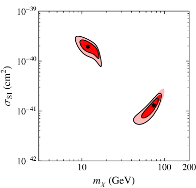
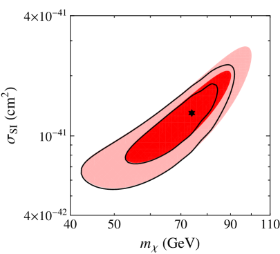
Figure 3: The preferred region of DAMA at 90% CL and 3$\sigma$ with (black contours) and without (dark and light red regions) GF using energy binned data on the amplitude and the phase of a cosine function fit to DAMA data. The left panel shows the result for a large range of dark matter masses, while the right panel zooms on the mass region where GF is important. The black star shows the best fit location with GF.

The results of this fit are shown in Fig. 3. Thanks to the energy spectrum information we obtain the two islands corresponding to scattering on sodium (low mass) and iodine (high mass). Again the effect of GF is to constrain more the high-mass edge of the iodine region. The difference of the regions with and without GF is smaller than in Fig. 2, because due to the energy information the region without GF is already more constrained towards high DM masses.

As mentioned above, the DM explanation of DAMA is in strong tension with exclusion limits from other experiments. In particular, the region around 80 GeV is excluded by the most recent limit from LUX [11] by around 4 orders of magnitude. In the following we are going to discard the DAMA signal and discuss annual modulation and GF in the context of a hypothetical future large scale direct detection experiment.

4 Annual modulation and GF in a future large scale experiment

4.1 Simulation details and event numbers

Let us assume that dark matter is just around the corner, slightly below the current best limit from the LUX experiment [11] and investigate how the signal of GF would look like in a future large scale direct detection experiment. To be specific, we assume a liquid xenon detector, inspired by upgrade plans of the XENON [12, 13] and LUX [15] collaborations, and the DARWIN consortium [14]. DARWIN is supposed to be the “ultimate” direct detection experiment, and exposures of order 10 ton yr are considered. As we will see in the following, it will be extremely difficult to establish an annual modulation signal, given the current constraints on the scattering cross section. Therefore, we are going to be very aggressive and assume an exposure of $10^{8}$ kg day $\approx 270$ ton yr. This corresponds roughly to a factor $10^{4}$ larger than the current LUX exposure, and could be achieved for instance by a $\sim 10$ yr exposure of a hypothetical $\sim 30$ ton detector. We stress that such a huge exposure goes beyond the currently discussed options. However, as we will see, even with those (probably unrealistic) assumptions it will be hard to establish statistically significant signals. Our results are easily scalable to any exposure.

Further assumptions of our simulated setup are motivated by the LUX and XENON100 analyses. For the detection efficiency we multiply together the blue and dotted green curves in Fig. 1 of Ref. [25]. Those curves are energy dependent, and give the combined cut acceptance for the XENON100 detector, corresponding to a hard discrimination cut used for the maximum gap method analysis. The final efficiency is roughly 30% for a large part of the energy interval we consider; at 3 keV, the efficiency is 8%, but reaches a value of 20% already at 4.5 keV. Our default energy interval is $[3,30.5]$ keV, where the threshold is motivated by the LUX analysis[11], but we show also results for $[6.5,30.5]$ keV, corresponding to the benchmark energy interval of the XENON100 experiment [25]. We adopt a Gaussian energy resolution with width of $0.1\sqrt{E_{nr}/E_{thr}}$ keV, where $E_{thr}$ is our chosen threshold energy. This is a very optimistic assumption on the energy resolution, however, we have checked that our results are very insensitive to the assumed energy resolution.

DM mass [GeV]	20	50	80	100	200
# events (no GF)	11305	21094	16974	14514	8058
# events (with GF)	11525	21418	17213	14712	8162

Table 1: Number of events with and without GF in our assumed xenon detector in the nuclear recoil energy range $[3.0,30.5]$ keV with an exposure of $270$ ton yr for $\sigma_{\rm SI}=10^{-45}$ cm² and various values of the DM mass.

We assume now a reference value for the spin-independent cross section of $\sigma_{\rm SI}=10^{-45}$ cm², close to the present upper limit. In Tab. 1 we give the total number of events predicted with and without GF for our adopted configuration. We expect of order $10^{4}$ events, with some dependence on the DM mass. The effect of GF on the total event numbers is very small (and degenerate with the scattering cross section or other global normalization factors, such as e.g., $\rho_{\infty}$).

4.2 The annual modulation signal with and without GF

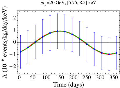
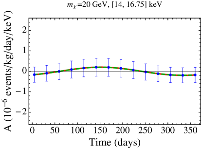
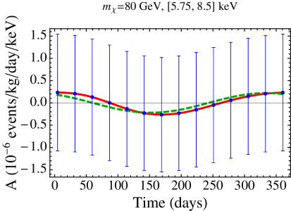
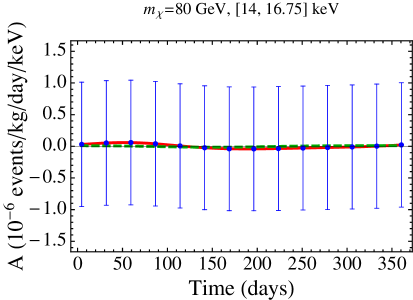
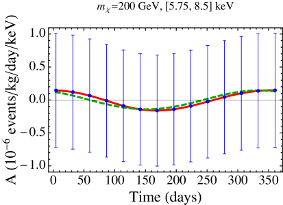
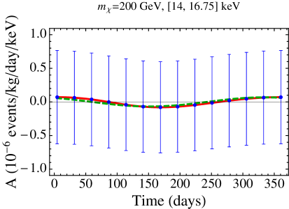
Figure 4: The annual modulation signal $A_{[E_{1},E_{2}]}/MT$, see Eq. (2.12), with GF (blue points and red curve) and without GF (green dashed curve) for a xenon target and a spin-independent cross section of $\sigma_{\rm SI}=10^{-45}$ cm². In the top, center, and bottom panels, $m_{\chi}=20$, 80, and 200 GeV, respectively. In the left and right panels, the energy interval chosen is $[5.75,8.5]$ keV and $[14,16.75]$ keV, respectively. Error bars correspond to the statistical error in $A_{[E_{1},E_{2}]}/MT$ including GF assuming an exposure of $MT=10^{8}$ kg day $\approx 270$ ton yr. Note the different scales on the vertical axes.

Let us now consider the size of the annual modulation signal for the setup described above. In Fig. 4 we show plots of $A_{[E_{1},E_{2}]}/MT$ (in events/kg/day/keV), where we divide the modulation amplitude given in Eq. (2.12) by the exposure $MT$, as a function of time for two different energy bins (of equal size). The blue points as well as the red curve show the predicted annual modulation signal with GF, and the error bars show their statistical error averaged over each time bin. The green dashed curve shows the annual modulation without GF. In the upper panels we assume a DM mass of 20 GeV. In this case the predicted signals with and without GF are identical. For such small masses we are probing large values of $v_{m}$ (364 km/s and 535 km/s in the center of the low and high energy bins in the left and right upper panels of Fig. 4, respectively), and in that region GF is negligible, compare to Fig. 1. Some differences in the predictions are visible in the middle and bottom panels, corresponding to DM masses of 80 and 200 GeV, respectively, and hence lower values of $v_{m}$ where GF becomes important. Considering the size of the error bars, it is clear that establishing GF – or even the annual modulation itself – at high significance will turn out to be hard. We will come back to this question below in subsection 4.3. Note that in the high-energy bin for $m_{\chi}=80$ GeV (right-middle panel) the modulation amplitude is very small. In this case we are very close to the phase flip ($v_{m}=190$ km/s in the center of the bin) where the amplitude is suppressed.

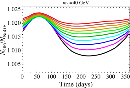
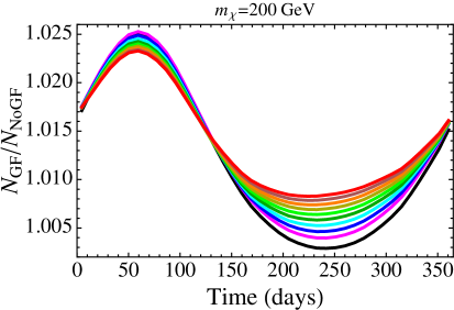
Figure 5: The ratio of the number of events with and without GF as a function of time and in different energy bins. The black to red curves correspond to energy bins of equal size in the interval of $[3.0,30.5]$ keV from lowest to highest, respectively. The left and right panels are for $m_{\chi}=40$ GeV and 200 GeV, respectively. We use a Gaussian energy resolution with a width of $0.1\sqrt{E_{nr}/3.0}$ keV.

Fig. 5 shows the ratio of the number of events with GF, $N_{\rm GF}$, and without GF, $N_{\rm NoGF}$, as a function of time and in different energy bins for the two values of the DM mass of 40 GeV and 200 GeV. The 10 colored lines correspond to 10 energy bins of equal size in the interval of $[3.0,30.5]$ keV starting from the lowest energy bin (black) to the highest one (red). Fig. 5 shows that the effect of GF is smaller for $m_{\chi}=40$ GeV compared to $m_{\chi}=200$ GeV. For both DM masses, the ratio is close to 1, with the size of the effect at the percent level.

4.3 Statistical significance of modulation and GF

We proceed now by estimating the achievable statistical significance for the annual modulation as well as for GF obtainable by our hypothetical xenon detector with an exposure of $MT\approx 270$ ton yr, as described in section 4.1. Again we take as reference value a cross section close to the present LUX bound of $\sigma_{\rm SI}=10^{-45}$ cm². We divide the “data” into 40 time bins per year and 10 energy bins of equal size in the energy interval of either $[3,30.5]$ keV or $[6.5,30.5]$ keV (in order to illustrate the importance of the threshold energy). Then we construct a $\chi^{2}$ function based on the annual modulation amplitude as defined in Eq. (2.12):

$$\Delta\chi^{2}(m_{\chi},\sigma_{\rm SI};\,m_{\chi}^{0},\sigma_{\rm SI}^{0})=\sum_{i,j}\left(\frac{A_{ij}^{\rm pred}(m_{\chi},\sigma_{\rm SI})-A_{ij}^{\rm obs}(m_{\chi}^{0},\sigma_{\rm SI}^{0})}{\sigma_{ij}}\right)^{2},$$ (4.1)

where the sum is over both time and energy bins, and $\sigma_{ij}$ is the statistical error of $A_{ij}^{\rm obs}$. Here, $A_{ij}^{\rm obs}$ plays the role of the future “data”, for which we take the predicted modulation amplitude for some particular “true” parameter values $(m_{\chi}^{0},\sigma_{\rm SI}^{0})$, where we fix $\sigma_{\rm SI}^{0}=10^{-45}$ cm² as mentioned above, but vary the assumed true DM mass $m_{\chi}^{0}$. Note that we do not include statistical fluctuations in our “data”, but instead use the most probable outcome of the experiment as data. This is sometimes called “Asimov data set” [26] and $\chi^{2}$ values obtained in this way describe the significance of the “average” experiment, see for instance [27] for an application of this approach in the dark matter context.

First we estimate the significance with which the presence of annual modulation can be established. To this aim we calculate the “data” $A_{ij}^{\rm obs}$ as described above for a choice of $m_{\chi}^{0}$ and our reference cross section, including GF. The $\chi^{2}$ value obtained then by fitting these data with a prediction constant in time will measure the significance of the modulation. Hence we set $A_{ij}^{\rm pred}=0$ in Eq. (4.1):

$$\Delta\chi^{2}_{\rm mod}(m_{\chi}^{0},\sigma_{\rm SI}^{0})=\sum_{i,j}\left(\frac{A_{ij}^{\rm obs}(m_{\chi}^{0},\sigma_{\rm SI}^{0})}{\sigma_{ij}}\right)^{2}\,.$$ (4.2)

Evaluating $\Delta\chi^{2}_{\rm mod}(m_{\chi}^{0},\sigma_{\rm SI}^{0})$ for 1 degree of freedom corresponds to the average significance for annual modulation, and hence, $\sqrt{\Delta\chi^{2}_{\rm mod}(m_{\chi}^{0},\sigma_{\rm SI}^{0})}$ gives the corresponding number of Gaussian standard deviations. The result of this analysis is shown with solid curves in the left panel of Fig. 6 for two different choices of energy threshold. For the black curve we use the energy interval $[3,30.5]$ keV, whereas for the green curve we use $[6.5,30.5]$ keV. We conclude from this figure that only in the mass range $m_{\chi}\lesssim 40$ GeV a significant ($>3\sigma$) signal for annual modulation can be obtained, whereas for larger DM masses only a hint below $2\sigma$ can be reached, despite the huge exposure we are assuming.

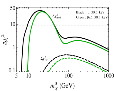
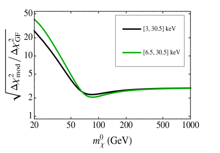
Figure 6: Left: The $\Delta\chi^{2}_{\rm mod}$ (Eq. (4.2)) is shown as a function of $m_{\chi}^{0}$ by solid lines. The dashed lines show the $\Delta\chi^{2}_{\rm GF}$ computed from Eq. (4.1) assuming the predicted signal is without GF. Right: The square root of the ratio $\Delta\chi^{2}_{\rm mod}/\Delta\chi^{2}_{\rm GF}$ as a function of $m_{\chi}^{0}$. We use an energy threshold of 3.0 keV and 6.5 keV for the black and green curves, respectively. We assume $\sigma_{\rm SI}=10^{-45}$ cm² and an exposure of $10^{8}$ kg day $\approx 270$ ton yr.

Next we want to estimate the significance of gravitational focusing. We formulate this in terms of a hypothesis test, where the presence of GF is the null hypothesis which we want to test against the alternative hypothesis of the absence of GF. Given data, one would perform a fit with and without GF and compute a test statistic $T$, for instance $T=\chi^{2}_{\text{with GF}}-\chi^{2}_{\text{without GF}}$. One can show that in the Gaussian approximation $T$ will be normal distributed with mean $T_{0}$ and standard deviation $2\sqrt{T_{0}}$ with $T_{0}=\Delta\chi^{2}_{\rm GF}$, where $\Delta\chi^{2}_{\rm GF}$ is obtained from Eq. (4.1) by calculating $A_{ij}^{\rm obs}$ including GF and the predicted signal, $A_{ij}^{\rm pred}$, without GF. A detailed discussion of the statistical method is given in Ref. [28], where a similar method is applied to the problem of identifying the neutrino mass ordering. In that reference also a derivation of the normal distribution of $T$ can be found. Following Ref. [28], we note that $\sqrt{\Delta\chi^{2}_{\rm GF}}$ corresponds to good approximation to the number of standard deviations with which the median experiment can reject the alternative hypothesis. The dashed curves in the left panel of Fig. 6 show the $\Delta\chi^{2}_{\rm GF}$ as a function of $m_{\chi}^{0}$. The black and green curves are for an energy threshold of 3 keV and 6.5 keV, respectively. We conclude that for our assumed setup the significance of detecting gravitational focusing never reaches the 1$\sigma$ level.

Note that our analysis is based on statistical errors only. This implies that all our $\chi^{2}$ values are proportional to the overall event normalization, and therefore scale linearly with the exposure $MT$ times the scattering cross section $\sigma_{\rm SI}^{0}$. Hence the curves in the left panel of Fig. 6 can easily be translated to any other exposure and/or cross section. In view of this observation we show in the right panel of Fig. 6 the quantity $\xi\equiv\sqrt{\Delta\chi^{2}_{\rm mod}/\Delta\chi^{2}_{\rm GF}}$. This number can be interpreted in the following way: assume that a future experiment established annual modulation at $n\sigma$ significance; then GF will be detected at a significance of $(n/\xi)\sigma$. The ratio $n/\xi$ is largest when $\Delta\chi^{2}_{\rm GF}$ reaches a maximum and $\Delta\chi^{2}_{\rm mod}$ reaches a local minimum, which happen at $m_{\chi}^{0}\sim 70-90$ GeV depending on the choice of energy threshold. This behavior is easy to understand, since as mentioned above, for those masses the phase flip of the modulation is located in the middle of the energy spectrum. This minimizes the amplitude of the modulation and explains the local minimum in the $\chi^{2}_{\rm mod}$ in the left panel (see also right-middle panel in Fig. 4), whereas around the phase flip the impact of GF on the phase of the modulation is strongest (see Fig. 1).

One might ask if the results are dependent on the choice of the number of time or energy bins in the calculation of $\Delta\chi^{2}$. We have checked that the significance of detecting the annual modulation and GF stay the same for various choices of the number of time and energy bins, as long as they are larger than a few. In particular, we observe that the energy spectrum seems not to be very important for our results. Thus the choice of 10 energy bins and 40 time bins give accurate results. This conclusion may change in the presence of systematic uncertainties and/or backgrounds, since in this case the particular energy shape of the signal may be important to limit the impact of such uncertainties. We have also checked that our choice of energy resolution is not crucial for our results.

To conclude this section we give two examples of the preferred regions in the DM mass–cross section plane obtainable from the annual modulation signal in our hypothetical future xenon detector. We calculate the “data” $A^{\rm obs}$ in Eq. (4.1) for two example values of the DM mass, 40 and 80 GeV, and the reference cross section $10^{-45}$ cm². Allowed regions can then be obtained by considering contours of $\Delta\chi^{2}$ from Eq. (4.1) in the $(m_{\chi},\sigma_{\rm SI})$ plane, as shown in Fig. 7. The “data” $A^{\rm obs}$ has been calculated including GF. In the figure we show the allowed regions for either including GF when calculating the prediction (black contour curves) or neglecting GF (colored regions). In the first case the $\chi^{2}$ minimum at the true parameter point is zero, whereas in the second case the minimum $\chi^{2}$ is non-zero (though very small, compare to Fig. 6). In this case contour levels are defined with respect to the (non-zero) minimum. As it can be seen from Fig. 7, GF affects only marginally the allowed region at 40 GeV, as expected from Fig. 6 and the observation that large $v_{m}$ values are probed for small DM masses. The difference for the $1\sigma$ region at 80 GeV looks striking, being closed from below (open) with (without) GF. There is no need to emphasize, however, that $1\sigma$ regions in general are not statistically meaningful, and already at $2\sigma$ the regions with and without GF are very similar.

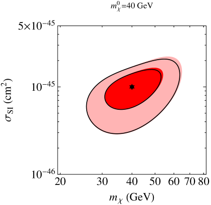
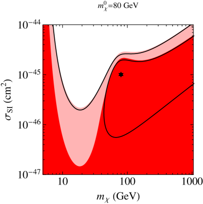
Figure 7: The preferred regions at 1$\sigma$ and 2$\sigma$ based on the annual modulation signal in a future xenon experiment with an exposure of 270 ton yr with GF (black contours) and without GF (dark and light red regions). In the left and right panels, we assume a positive signal at $m_{\chi}^{0}=40$ GeV, and 80 GeV, respectively, both with a cross section of $10^{-45}$ cm², as specified with a star in the plots.

Let us stress that here we discard any information on the absolute number of events and base the regions only on the annual modulation signal. Clearly, with event numbers of order $10^{4}$ in our setup (see Tab. 1) in principle a very precise mass and cross section determination will be possible, assuming that backgrounds as well as astrophysical uncertainties are under control, see e.g., Ref. [27] for analyses along those lines in the context of DARWIN. The purpose of the discussion here is to investigate the potential (or the lack thereof) of the annual modulation signal, which is supposed to be more robust against systematic uncertainties.

4.4 Comments on light targets

Let us briefly comment also on lighter target nuclei and experiments aiming at very low threshold, such as for instance the CDMSlite experiment [29]. In this case in principle somewhat lower $v_{m}$ values are probed even for light DM, where the modulation amplitude is larger. Therefore, a valid question is whether GF becomes more important for such configurations. We have performed similar tests as the one described above for a Xe detector also for setups using Ar and Ge. In general the signal is reduced compared to Xe (for the same nucleon cross section and exposure) due to the $A^{2}$ dependence of the rate. However, the shape of the curves for $\Delta\chi^{2}_{\rm mod}$ and $\Delta\chi^{2}_{\rm GF}$ as a function of $m_{\chi}$ are similar to the case of xenon. In particular, for an argon detector (with threshold 3 keV) we obtain a very similar result for the ratio shown in the right panel of Fig. 6.

The germanium based experiment CDMSlite [29] has achieved a threshold of 0.84 keV. This opens the possibility to test very low DM masses, where the modulation signal can be very significant. We tested a hypothetical Ge detector with a threshold of 0.84 keV and again we arrive at qualitatively similar conclusions as for Xe. For example, for a DM mass of 4 GeV we can take a cross section of $10^{-40}$ cm², just below the current limits. In this case we would need an exposure of about $10^{6}$ kg day in order to see a $3\sigma$ effect of GF ($\Delta\chi^{2}_{\rm GF}\sim 10$). This assumes a background free experiment and has to be compared to the current CDMSlite exposure of about 6 kg day [29].

4.5 Comments on inelastic scattering

Above we focused exclusively on elastic spin-independent scattering. Let us comment briefly on other particle physics scenarios. We do not expect any qualitative change for other DM–nucleus interactions, which provide some kind of re-scaling of the scattering rate, such as spin-dependent scattering or couplings of different strength to neutrons and protons. There may be, however, non-trivial effects for interaction types which modify the kinematics and/or change the ratio of the amplitude of the annual modulation to the time-constant signal. One example of this type is inelastic scattering, $\chi+A\to\chi^{\prime}+A$, with the mass difference $\delta=m_{\chi^{\prime}}-m_{\chi}$. In this case the expression for the minimal velocity, Eq. (2.2), is changed to

$$v_{m}=\frac{1}{\sqrt{2m_{A}E_{nr}}}\left|\frac{m_{A}E_{nr}}{\mu_{\chi A}}+\delta\right|.$$ (4.3)

In the case of endothermic scattering, $\delta>0$, the DM particle up-scatters to an excited state [30]. In this case scattering off heavier target nuclei is favored. It is clear from Eq. (4.3) that for $\delta>0$, $v_{m}$ gets larger compared to the elastic case, and hence, we expect that GF becomes less important (c.f. Fig. 1). Indeed, we find that for endothermic scattering the significance of detecting GF is very small, and $\Delta\chi^{2}_{\rm GF}$ never reaches even 0.1 for our setup.

On the other hand, if $\delta<0$, the DM particle down-scatters to a lower mass state, which is called exothermic scattering [31, 32, 33], and in this case we are probing the region of smaller $v_{m}$ where GF can be important. The significance of detecting the annual modulation and GF are shown in the left and right panels of Fig. 8, respectively, for different choices of negative $\delta$. Here we again assume a Xe detector as described in section 4.1. The case of elastic scattering ($\delta=0$) is also shown in dashed black. As one can see from the right panel of Fig. 8, the significance of detecting GF can reach values above 1$\sigma$ for $|\delta|\gtrsim 20$ keV.

The wiggles at low masses in the $\Delta\chi^{2}_{\rm mod}$ curves for negative $\delta$ (most pronounced for $\delta=-80$ keV) occur when $v_{m}$ goes through zero for different energy bins, see Eq. (4.3) for $\delta<0$. For the WIMP mass and recoil energy at which $v_{m}=0$, we are integrating the velocity distribution over a large range of velocities, which leads to a small amplitude for the annual modulation. Thus for such masses, $\Delta\chi^{2}_{\rm mod}$ goes through a local minimum and the significance of detecting the annual modulation is smaller.

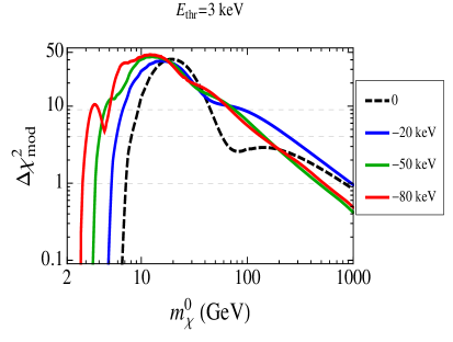
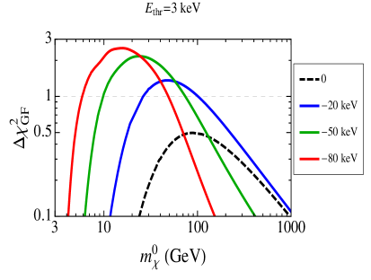
Figure 8: The $\Delta\chi^{2}_{\rm mod}$ (left) and the $\Delta\chi^{2}_{\rm GF}$ (right) for inelastic exothermic scattering, shown as a function of $m_{\chi}^{0}$ using an energy threshold of 3.0 keV. The dashed black curve corresponds to the elastic case ($\delta=0$), while the other colors correspond to different values of $\delta<0$. We assume $\sigma_{\rm SI}=10^{-45}$ cm² and a Xe exposure of $270$ ton yr.

5 Summary

In this paper we have considered the impact of the Sun’s gravitational potential on the annual modulation signal in dark matter direct detection experiments. The distortion of the DM phase space distribution due to the gravitational focusing (GF) of the Sun may potentially lead to a significant modification of the time dependence of the count rate [7]. To illustrate the importance of this effect we have considered the signal reported by the DAMA/LIBRA experiment. Performing a fit to their time dependent data we find that the allowed DM parameter range is more restricted (for large DM masses) if the effect of GF is taken into account. Since, however, for those DM masses the relevant cross section is excluded by many orders of magnitude by recent constraints from other experiments, we set the DAMA/LIBRA signal aside and investigate the potential of possible future large-scale direct detection experiments.

We consider a very large xenon-based setup, with an exposure around $10^{4}$ times larger than the current exposure from the LUX experiment [11], corresponding to about 270 ton yr. Furthermore, we assume that DM is just around the corner, with a DM–nucleus cross section of $\sigma_{\rm SI}=10^{-45}$ cm², roughly at the present LUX exclusion limit. Even under those very optimistic assumptions our results indicate that most likely the answer to the question posed in the title of the paper is “no”. We find that an annual modulation signal can be established at a significance of $\gtrsim 3\sigma$ only for DM masses $m_{\chi}\lesssim 40$ GeV. For such small masses, only the high-velocity tail of the DM distribution is probed, where the effect of GF is very small. In the region of larger DM masses, where GF may be potentially observable, the annual modulation signal itself will not become significant. We have considered also the case of inelastic scattering, where for the exothermic case (down-scattering) the effect of GF is slightly larger than for the elastic case, because of the lower DM velocities involved. We have also checked that our conclusions hold in case of lighter target nuclei such as Ar and Ge.

Our calculations are based on the Standard Halo Model, corresponding to an isotropic Maxwellian velocity distribution. It is well known that deviations from this halo may have important consequences for the annual modulation signal [34, 17, 35]. Investigating the impact of GF in the presence of more complicated DM velocity distributions, such as streams or debris flows is beyond the scope of this work. Generically we do not expect that the size of the GF effect will change, however, we cannot exclude the possibility that particular configurations, for instance a dark disk, may enhance the importance of GF. It might be a hard task to disentangle GF effects from non-standard halos. In general, we conclude by noting that for a given halo model the impact of GF is determined and calculable, and in case of doubt should be included in the analysis.

Acknowledgements

N.B. acknowledges discussions with Graciela Gelmini about investigating the impact of gravitational focusing on the DAMA regions during the TAUP 2013 conference. We thank the authors of Ref. [7] for valuable comments on the first version of this paper. We acknowledge support from the European Union FP7 ITN INVISIBLES (Marie Curie Actions, PITN-GA-2011-289442). N.B. thanks the Oskar Klein Centre and the CoPS group at the University of Stockholm for hospitality during her long-term visit.

References

- [1] K. Griest, Effect of the Sun’s Gravity on the Distribution and Detection of Dark Matter Near the Earth, Phys.Rev. D37, 2703 (1988).
- [2] P. Sikivie and S. Wick, Solar wakes of dark matter flows, Phys.Rev. D66, 023504 (2002), astro-ph/0203448.
- [3] M. S. Alenazi and P. Gondolo, Phase-space distribution of unbound dark matter near the Sun, Phys.Rev. D74, 083518 (2006), astro-ph/0608390.
- [4] B. R. Patla, R. J. Nemiroff, D. H. H. Hoffmann, and K. Zioutas, Flux Enhancement of Slow-moving Particles by Sun or Jupiter: Can they be Detected on Earth?, Astrophys.J. 780, 158 (2014), 1305.2454.
- [5] J. M. A. Danby and G. L. Camm, Statistical dynamics and accretion, MNRAS 117, 50 (1957).
- [6] J. M. A. Danby and T. A. Bray, Density of interstellar matter near a star, Astron.J. 72, 219 (1967).
- [7] S. K. Lee, M. Lisanti, A. H. G. Peter, and B. R. Safdi, Effect of Gravitational Focusing on Annual Modulation in Dark-Matter Direct-Detection Experiments, Phys.Rev.Lett. 112, 011301 (2014), 1308.1953.
- [8] A. K. Drukier, K. Freese, and D. N. Spergel, Detecting Cold Dark Matter Candidates, Phys. Rev. D33, 3495 (1986).
- [9] K. Freese, J. A. Frieman, and A. Gould, Signal Modulation in Cold Dark Matter Detection, Phys. Rev. D37, 3388 (1988).
- [10] DAMA/LIBRA Collaboration, R. Bernabei et al., New results from DAMA/LIBRA, Eur.Phys.J. C67, 39 (2010), 1002.1028.
- [11] LUX Collaboration, D. S. Akerib et al., First results from the LUX dark matter experiment at the Sanford Underground Research Facility, 1310.8214.
- [12] XENON1T collaboration, E. Aprile, The XENON1T Dark Matter Search Experiment, (2012), 1206.6288.
- [13] G. Plante, The Multi-Ton XENON Program at the Gran Sasso Laboratory, talk at Dark Matter 2014, UCLA, http://www.pa.ucla.edu/sites/default/files/webform/plante-dm2014-20140228.pdf.
- [14] DARWIN Consortium, L. Baudis, DARWIN: dark matter WIMP search with noble liquids, J.Phys.Conf.Ser. 375, 012028 (2012), 1201.2402.
- [15] D. Malling et al., After LUX: The LZ Program, (2011), 1110.0103.
- [16] G. Gelmini and P. Gondolo, WIMP annual modulation with opposite phase in Late-Infall halo models, Phys.Rev. D64, 023504 (2001), hep-ph/0012315.
- [17] A. M. Green, Effect of realistic astrophysical inputs on the phase and shape of the WIMP annual modulation signal, Phys. Rev. D68, 023004 (2003), astro-ph/0304446.
- [18] C. McCabe, The Earth’s velocity for direct detection experiments, JCAP 1402, 027 (2014), 1312.1355.
- [19] S. K. Lee, M. Lisanti, and B. R. Safdi, Dark-Matter Harmonics Beyond Annual Modulation, JCAP 1311, 033 (2013), 1307.5323.
- [20] S. Chang, J. Pradler, and I. Yavin, Statistical Tests of Noise and Harmony in Dark Matter Modulation Signals, Phys.Rev. D85, 063505 (2012), 1111.4222.
- [21] R. Bernabei et al., New limits on WIMP search with large-mass low-radioactivity NaI(Tl) set-up at Gran Sasso, Phys. Lett. B389, 757 (1996).
- [22] M. Fairbairn and T. Schwetz, Spin-independent elastic WIMP scattering and the DAMA annual modulation signal, JCAP 0901, 037 (2009), 0808.0704.
- [23] N. Bozorgnia, R. Catena, and T. Schwetz, Anisotropic dark matter distribution functions and impact on WIMP direct detection, JCAP 1312, 050 (2013), 1310.0468.
- [24] S. Chang, A. Pierce, and N. Weiner, Using the Energy Spectrum at DAMA/LIBRA to Probe Light Dark Matter, Phys.Rev. D79, 115011 (2009), 0808.0196.
- [25] XENON100 Collaboration, E. Aprile et al., Dark Matter Results from 225 Live Days of XENON100 Data, Phys.Rev.Lett. 109, 181301 (2012), 1207.5988.
- [26] G. Cowan, K. Cranmer, E. Gross, and O. Vitells, Asymptotic formulae for likelihood-based tests of new physics, Eur.Phys.J. C71, 1554 (2011), 1007.1727.
- [27] J. L. Newstead, T. D. Jacques, L. M. Krauss, J. B. Dent, and F. Ferrer, The Scientific Reach of Multi-Ton Scale Dark Matter Direct Detection Experiments, Phys.Rev. D88, 076011 (2013), 1306.3244.
- [28] M. Blennow, P. Coloma, P. Huber, and T. Schwetz, Quantifying the sensitivity of oscillation experiments to the neutrino mass ordering, JHEP 1403, 028 (2014), 1311.1822.
- [29] SuperCDMSSoudan Collaboration, R. Agnese et al., CDMSlite: A Search for Low-Mass WIMPs using Voltage-Assisted Calorimetric Ionization Detection in the SuperCDMS Experiment, Phys.Rev.Lett. 112, 041302 (2014), 1309.3259.
- [30] D. Tucker-Smith and N. Weiner, Inelastic dark matter, Phys. Rev. D64, 043502 (2001), hep-ph/0101138.
- [31] D. P. Finkbeiner and N. Weiner, Exciting dark matter and the INTEGRAL/SPI 511 keV signal, Phys. Rev. D76, 083519 (2007), astro-ph/0702587.
- [32] B. Batell, M. Pospelov, and A. Ritz, Direct detection of multi-component secluded WIMPs, Phys. Rev. D79, 115019 (2009), 0903.3396.
- [33] P. W. Graham, R. Harnik, S. Rajendran, and P. Saraswat, Exothermic dark matter, Phys. Rev. D82, 063512 (2010), 1004.0937.
- [34] N. Fornengo and S. Scopel, Temporal distortion of annual modulation at low recoil energies, Phys. Lett. B576, 189 (2003), hep-ph/0301132.
- [35] K. Freese, M. Lisanti, and C. Savage, Annual Modulation of Dark Matter: A Review, Rev.Mod.Phys. 85, 1561 (2013), 1209.3339.